DEVELOPMENT OF EXPOSOME CORRELATION GLOBES TO MAP OUT ENVIRONMENT-WIDE ASSOCIATIONS

Abstract

The environment plays a major role in influencing diseases and health. The phenomenon of environmental exposure is complex and humans are not exposed to one or a handful factors but potentially hundreds factors throughout their lives. The exposome, the totality of exposures encountered from birth, is hypothesized to consist of multiple inter-dependencies, or correlations, between individual exposures. These correlations may reflect how individuals are exposed. Currently, we lack methods to comprehensively identify robust and replicated correlations between environmental exposures of the exposome. Further, we have not mapped how exposures associated with disease identified by environment-wide association studies (EWAS) are correlated with other exposures. To this end, we implement methods to describe a first “exposome globe”, a comprehensive display of replicated correlations between individual exposures of the exposome. First, we describe overall characteristics of the dense correlations between exposures, showing that we are able to replicate 2,656 correlations between individual exposures of 81,937 total considered (3%). We document the correlation within and between broad a priori defined categories of exposures (e.g., pollutants and nutrient exposures). We also demonstrate utility of the exposome globe to contextualize exposures found through two EWASs in type 2 diabetes and all-cause mortality, such as exposure clusters putatively related to smoking behaviors and persistent pollutant exposure. The exposome globe construct is a useful tool for the display and communication of the complex relationships between exposure factors and between exposure factors related to disease status.

1. Introduction

1.1. A need to identify correlations between exposures

The environment is hypothesized to play a significant role in health and disease, but we lack methods to elucidate how multiple environmental exposures are associated together with disease. Along this line, Wild and Rappaport and Smith have documented a new way to conceptualize the environment called the “exposome” [1, 2], the environmental analog of the genome that consists of the totality of exposures from birth to death. Recently, others and we have proposed a new method to search for environmental factors associated with disease called the environment-wide association study (EWAS) (e.g.,[3-6]). EWAS is analytically analogous to the genome-wide association study (GWAS), a comprehensive way to search for genetic variants associated with disease.

While EWAS and GWAS are operationally similar, genotypes and exposures are very different data types and correlation structures. Genotypes are static and often assume a fixed number of discrete values (e.g., homozygous/heterozygous for single nucleotide polymorphisms). Correlation between genetic variants is a function of chromosomal location due to the phenomenon of “linkage disequilibrium” (LD). The closer variants are located along the genome, the greater the chance they will be inherited together and correlated.

On the other hand, environmental exposures are heterogeneous (in measurement modality and data type) and are dependent on geographic location, human behavior, and time. Their correlation is known to be “denser” than that of genetic variants [3, 7] as many exposures are correlated with many others [8, 9]. Importantly, given an exposure identified from an EWAS, it is very difficult to infer if the exposure is independently associated with the disease, the direction of association (“what causes what”), or if the exposure is simply a correlate [7, 9].

Given these challenges, it is a priority to develop methods to identify robust correlations between exposures. Correlation between exposures may allow investigators to describe how exposures can lead to other exposures (as identified in an EWAS). For example, many nutrients are consumed together. A non-optimal diet (however it may be defined) may lead to a deficiency in a whole group of vitamins and nutrients. As another example, individuals who are exposed to air pollution may have high levels of several products of combustion, including hydrocarbons, volatile compounds, and heavy metal levels. In the environmental health sciences it is hypothesized that prevalent “mixtures”, or combinations of exposures, may dictate health [10]; understanding how exposures are correlated is one step toward defining what mixtures are relevant to human health.

Many methods have been proposed to describe the correlation between multiple variables, often under the analytical category of “unsupervised learning”, and have been used successfully in the genomics field (e.g, [11-13]). We have yet to apply these methods to describe relationships between exposures. In this report, we describe correlations between exposure variables to construct an “exposome globe”, extending methods developed for unsupervised learning with genomic data called “relevance networks” [13]. We utilize the exposome globe to identify clusters of exposures correlated with exposures identified in EWAS (“EWAS-identified exposure”). We hypothesize it is possible to attain a broader and more interpretable view of EWAS-identified exposures with an exposome globe.

1.2. Methods

1.2.1. About the National Health and Examination Survey (NHANES) data

As documented earlier (e.g., [4]), we attained four NHANES surveys data each representing independent samplings from the US population in years 1999-2000, 2001-2002, 2003-2004, and 2005-2006. Each NHANES survey dataset ascertains an array of environmental factors, sociodemographic factors (e.g., income), and clinical indicators (e.g., serum glucose, time to death). NHANES is a representative sampling of the US population and therefore covers the entire age, sex, and demographic distribution of the US.

We constructed a correlation globe with factors of the exposome. These factors include direct and quantitative measurement of environmental exposures representing chemicals, nutrients, or infectious agents (assayed directly in human tissue, such as blood serum, urine and hair). For example, quantitative measurements of nutrient (e.g., vitamins, carotenes) and pollutant (e.g., heavy metals, polychlorinated biphenyls) levels in human tissue are ascertained via mass spectrometry (MS), such as gas chromatography and inductively coupled plasma MS. Infectious agents (e.g., bacteria) were measured via immunological assays. Second, the CDC ascertained other indicators of environmental exposure including participant self-reported nutrient consumption (derived from a food questionnaire on foods consumed prior to the interview), physical activity, and prescribed pharmaceutical drugs.

1.2.2. Construction of an exposome globe of replicated environmental correlations

Our method is similar to that of the “relevance network” framework to find correlations of expressed genes [13]. We computed the non-parametric correlation coefficient between each pair of environmental factors (e.g., biomarkers of exposures and self-reported information) for each independent survey (e.g., 1999-2000, 2001-2002, 2003-2004, and 2005-2006). These coefficients are bi-serial coefficients between pair of binary factors and Spearman correlations for continuous factors. There are many ways to compute correlations between variables. We chose a non-parametric metric as to not make any distributional assumptions regarding the environmental factors.

We computed 37,207 correlations in the 1999-2000 survey (we denote the set of all correlations by ρ^1999-2000), 59,412 in 2001-2002 (ρ^2001-2002), 128,715 in 2003-2004 (ρ^2003-2004) and 51,340 in 2005-2006 (ρ^2005-2006). We filtered out correlations that were present in only one survey and therefore could not be replicated and those that had sample sizes less than 10. After filtering, we were left with 35,835, 56,557, 80,401, 47,203 correlations in each of the four surveys respectively.

These correlations represented interdependencies between 289 unique environmental factors in 1999-2000, 357 in 2001-2002, 456 in 2003-2004, and 313 in 2005-2006 surveys. A total of 575 unique factors were observed across all surveys. The sample sizes for computing correlations ranged from 11 to 9965 (median 1883) in 1999-2000, 11 to 11,039 (median 2237) in 2001-2002, 11 to 10122 (median 2271) in 2003-2004, and 33 to 10348 (median 3267) in 2005-2006.

There were a different number of correlations measured in 2, 3, or 4 surveys. This is because the CDC had different sample sizes for different exposures. Specifically, 41,158 correlations were ascertained in 2 surveys (e.g., 1999-2000 and 2003-2004), 25,436 in 3 surveys (e.g., 1999-2000, 2003-2004, and 2005-2006), and 15,343 in all 4 surveys, resulting in a total of 81,937 correlations considered.

We used a permutation-based approach to estimate the two-sided p-value of significance for each pair of correlations within each independent survey. Specifically, each environmental factor was randomly permuted (sampled without replacement) and the correlations were re-computed to create a set of correlations that reflected the null distribution of no correlation. Briefly, given an exposure X and Y in one dataset of NHANES, we shuffled values of X to a new array X̃and computed the correlation between X̃ and Y. We repeated this procedure for all pairs of correlations for each survey. We denote distribution of correlations derived from the randomly permuted datasets as ${\tilde{\rho }}^{1999-2000},{\tilde{\rho }}^{2001-2002},{\tilde{\rho }}^{2003-2004},{\tilde{\rho }}^{2005-2006}$ for each of the 4 surveys respectively. The p-value for an individual correlation from ρ was the fraction of correlations from the permuted dataset $\tilde{\rho }$ with greater absolute value. For example, for a correlation ρ_x from ${\tilde{\rho }}^{1999-2000}$ the p-value equals ${\sum }_{i=1}^{35835}I(\mid {\rho }_x\mid <\mid {\tilde{\rho }}_i^{1999-2000}\mid )∕35835$ function.

We then estimated the false discovery rate (FDR) q-value for each correlation in each of the surveys using the Benjamini-Hochberg step-down approach [14], resulting in a vector of q-values for each survey, denoted as q^1999–2000, q^2001–2002, q^2003–2000, q^2003–2004, q^2005–2006,. We deemed a correlation to be replicated if its q-value was less than 5% in at least 2 surveys.

A replicated correlation can exist in 2, 3, or 4 independent dataset surveys. We computed a single “overall” correlation that summarized the correlation from multiple surveys with the inverse variance weighting method as used in fixed-effect meta-analyses[15]. In summary, we computed the overall coefficient as weighted average of the coefficients from each of the survey where weights are the standard errors of coefficient. The exposome globe consisted of overall summarized correlations in a set of tuples called P. Each tuple contains the relationship between exposures A and B and their correlation coefficient (ρ). Specifically, if a correlation between exposure A and B was replicated, its overall correlation is inserted in P as the tuple [(A, B), ρ], where (A, B) links A to B and ρ is the summarized correlation coefficient.

We visualized replicated overall correlations with the Circos visualization toolkit version 0.67 [16]. Each individual environmental factor is grouped and arranged in a circle. Lines between factors on the inside of the circle depict replicated correlations between factors and the thicknesses of the lines depict the absolute values of the correlations. Red and blue lines represent positive and negative correlations respectively.

1.2.3. Environment-wide association findings in type 2 diabetes and all-cause mortality

Previously, we have conducted EWASs for type 2 diabetes (T2D [4]) and all-cause mortality [5]. In T2D, we searched for association between 252 serum and urine biomarkers of exposure with serum fasting glucose and validated 10 factors. These 10 factors included nutrients such as trans/cis-β-carotene and vitamin C/D and pollutants such as PCB170 and heptachlor epoxide. In all-cause mortality, we searched for association between 249 environmental exposures and self-reported consumption behaviors and validated 7 factors, including urine-measured and serum-measured cadmium, smoking behaviors (e.g., number of cigarettes smoked per day), and physical activity behaviors (e.g., metabolic equivalents).

We visualized the EWAS findings from these studies in the exposome globe. First, we plotted the −log10(p-value) of association between the environmental factor and outcome (e.g., T2D, all-cause mortality) as a scatter plot in the Circos plot (referred to as an “EWAS track” below). Next, given a set E of validated factors (e.g. the 10 factors validated in T2D), we filtered and visualized correlations of pairs (A, B) from P that contained any factor in E (e.g., all pairs (E, B) or (A, E) where E is a validated exposure in E). In other words, we visualized all “first-degree neighbors” of the validated EWAS findings E from P.

2. Results

2.1. Distribution of correlations of the exposome globe

We considered 81,937 total correlations of the exposome. Correlations among factors of the exposome were modest; specifically, the median of the absolute value of all correlations was 0.025 (interquartile range of 0.010 to 0.06, Figure 1A [red line]).

Fig 1.

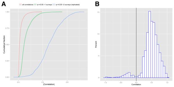
A.) Cumulative distribution of absolute value of correlations. The red line denotes the summarized correlation coefficients for all pairs of exposures possible. The green line denotes correlations that achieved q-value less than 5%. The blue line denotes correlations that were replicated (and part of the exposome globe), or had q-value less than 5% in at least 2 surveys. B.) Histogram of all replicated correlations of the exposome globe. Vertical black line denotes 0 correlation.

Of the 81,937 correlations, 12,385 (15%) had a q-value less than 5% in at least 1 survey dataset. Of these, the median absolute value of correlation was 0.122 (interquartile range of 0.071 to 0.282, Figure 1A [green line]).

We define the “exposome globe” as the network of correlations that were replicated (q-value less than 5% in at least two independent surveys). Of the 81,937 correlations, 2,656 (3%) were replicated and made up the exposome globe. The median absolute value of correlations of the exposome globe was markedly higher than the median of all correlations at 0.5 (interquartile range of 0.385 to 0.635, Figure 1A [blue line]). Most of the replicated correlations (2,513 of 2,656) had positive sign (Figure 1B). The median of positive and negative replicated correlations was 0.508 and −0.282 respectively (Figure 1B).

2.1.1. Concordance of replicated correlations

We observed that correlations were concordant between surveys. The concordance of the exposure correlations between the different surveys was greater than 0.8 (assessed via Pearson ρ, Table 1). For example, the concordance between all correlations in the 2001-2002 and the 2003-2004 survey was 0.82 (Table 1). All correlations were highly significant (p<10⁻¹⁰). As expected, when only considering replicated correlations (relationships of the exposome globe), the concordance was greater (e.g., concordance between 2001-2002 and 2003-2004 survey was 0.90). Therefore, while correlations were modest/small (Figures 1AB) they were reproducible across cohorts.

Table 1.

Pearson ρ of exposure correlations between each independent NHANES dataset. Number of correlations compared are in parentheses.

	1999-2000	2001-2002	2003-2004	2005-2006
1999-2000	1.00	0.84 (33191)	0.84 (34337)	0.92 (16955)
2001-2002		1.00	0.82 (55025)	0.93 (22931)
2003-2004			1.00	0.94 (47070)
2005-2006				1.00

2.1.2. The exposome globe reflects correlations within and between categories of factors

While the globe was dense (2,656 of all possible 81,937 correlations were replicated) we observed interpretable broad patterns in the exposome globe (Figure 2). First, we observed positive correlations within each exposure category (“intra-category” correlations), such as between serum nutrients, nutrients ascertained from food recall questionnaires, volatile organic compounds, hydrocarbons, polychlorinated biphenyls (PCBs), dioxins, phthalates, bacteria (co-infection), and pesticides. We observed positive correlations between categories of exposures, such as between phthalates and hydrocarbons, PCBs and dioxins, dioxins and furans, furans and PCBs, pesticides and PCBs. Of note, there were positive correlations between some nutrients and pollutants, such as PCBs, dioxins, and furans. Briefly, PCBs, dioxins, hydrocarbons, and furans are “persistent pollutants”. Persistent pollutants are lipophilic (accrue in fatty tissue) and accumulate in the food chain. PCBs had been used for manufacturing materials whose use has been banned during the 1970s. Dioxins, furans and hydrocarbons are by-products of industrial processes such as pesticide manufacturing and combustion. Demographic factors, including age, sex, and race/ethnicity were also correlated with multiple groups of exposures.

Fig 2. Overall Exposome Correlation Globe.

575 exposures are grouped by a priori defined environmental health categories and displayed in different colors in the globe. Replicated correlations are shown in red (positive correlation) or blue (negative correlation) lines between exposures. Line thickness is proportional to size of the absolute value of correlation coefficient. Only replicated correlation links are displayed (distribution shown in Figure 1B).

2.1.3. Describing EWAS-identified factors with the exposome globe

We used the exposome globe to describe the first-degree correlations of factors validated in previous EWAS investigations of T2D and all-cause mortality. We only selected correlation links in the exposome globe that were between validated EWAS exposures and other exposures. We observed qualitatively different globes for EWAS factors found in T2D and mortality (Figure 3).

Fig 3. A.) Exposome Correlation Globes for EWAS in All-Cause Mortality and B.) T2D.

Association p-values from EWAS are shown as a separate track (“EWAS track”) above each exposure (red points denote EWAS validated associations with positive effect size [indicating risk] blue points indicate an EWAS validated negative effect size [indicating protective]). Validated EWAS associations for T2D and all-cause mortality are offset in labeled in red or blue text. Only “first-degree” correlations (correlations for validated EWAS findings) are displayed in the globes and displayed in black text. Acryl.=acrylamide; Mel=Melamine; VoC=volatile organic compounds; PCBs=polychlorinated biphenyls; PFCs=polyfluorinated compounds

In all-cause mortality, we observed clusters of correlated exposures putatively related to smoking but little related to healthy behaviors, such as physical activity or diet (Figure 3A). Specifically, we observed that the self-reported variables of current and past smoking, which had been identified via EWAS as risk factors for death (red points in the EWAS track, Figure 3A), were correlated with hydrocarbons (e.g., napthols) and volatile organic compounds (e.g., toluene). Further still, urine and serum cadmium, both also positively associated with death (red points on the EWAS track), were also correlated with smoking status and a biomarker of nicotine (cotinine). There were relatively fewer correlates for factors that were associated with protection from death, such as trans lycopene and physical activity.

In T2D, we observed that serum measures of PCB170 and heptachlor epoxide, two types of banned and polychlorinated compounds used in materials manufacturing and pesticides respectively, and positively associated with T2D (red point in EWAS track [Figure 3B]), correlated with other exposures of the same category, such as other polychlorinated biphenyls and pesticides. Therefore, PCB170 and heptachlor epoxide could be a marker of correlated chlorinated exposures, all which may play a role in T2D. Cumulative role of groups of persistant pollutants is indeed one hypothesis for T2D [17]. Serum levels of Vitamin A (e.g., retinol, retinyl stearate, and retinyl palmitate), were positively correlated with heptachlor epoxide. Further, serum-measures of γ-tocopherol, a type of vitamin E (positive association with T2D, red point in EWAS track, Figure 3B), was negatively correlated with serum-measured folate (blue correlation line, Figure 3B); individuals with high levels of γ-tocopherol had lower levels of folate.

3. Discussion

3.1.1. Summary of findings

By relating all possible exposures with one another by comprehensively computing correlations and replicating these correlations across multiple independent survey datasets, we were able to produce a first exposome correlation globe. We observed that this globe contains many reproducible correlations between exposures of the same environmental health category or group, but also between these groupings. The correlations of these exposures may be indicative of ways human populations are exposed (“routes of exposure”), such as behaviors and/or shared metabolic fate of biomarkers of exposure. Relatedly and importantly, by selecting correlations that are related to a disease outcome and identified by EWAS (via the EWAS track), we can create hypotheses regarding disease-related exposures, such as smoking correlates in mortality and persistent pollutants in T2D.

3.1.2. Strengths of exposome globes

There are several advantages of the proposed exposome globes. First, exposome globes allow the presentation and visualization of the clusters of co-existing exposures, or mixtures, in humans. These mixtures may be a result of common routes of exposure or behaviors (e.g., foods are mixtures of nutrients or smoking behavior can result in a mixture of hydrocarbons and heavy metals). These systematic correlations may also help identify shared characteristics of exposures; for example, chlorinated persistent pollutants were all densely correlated with one another perhaps due to shared routes of exposure, but also because they happen to be lipophilic and have similar metabolic fates.

Secondly, knowing how exposures are correlated with one another may aid inference in disease association studies, such as EWAS or gene-environment (GxE) interaction studies. For example, displaying EWAS identified factors with correlation globes may enable investigators to pin down behaviors that underlie the correlations. For example, we observed that many of the exposures found in an EWAS in all-cause mortality, such as smoking, were strongly correlated with hydrocarbons and volatile organic compounds. These compounds may be indicative of the complex chemical matrix of cigarette smoke (e.g., metals, hydrocarbons, and volatile compounds may be found in cigarette smoke). Such a visualization is analogous to a “manhattan plot” in GWAS, where the correlation (LD) between genetic variants and their p-value of association is visualized jointly to enable assessment of independence of associations between genotype and disease [18].

Relatedly, in GxE investigations, exposome globes may present alternative scenarios for interaction between the environment and genetic variants. Because of power and sample size constraints, GxE investigations test a few environmental factors at a time [19]. For example, we recently documented an interaction between serum levels of trans-β-carotene and a GWAS-identified SNP, rs13266634 in the SLC30A8 gene in T2D [20]. However, evidence of statistical interaction is not evidence of biological interaction. But, other exposures correlated with trans-β-carotene (e.g., Figure 3B) may provide clues to other possible alternative molecular pathways that are centered on the SLC30A8 gene.

Third, correlated exposures may enable investigators to identify biases, such as confounders in association studies, including EWAS or GxE interaction studies. Confounded exposures are those that are not causal, but associated with the disease of interest (e.g., diabetes or mortality) and the causal exposure (similar to genetic loci in linkage as discussed above). Once correlated exposures are identified through the globe, investigators can attempt to “control” and condition for them in their statistical models to observe how they influence the strength of association between exposures and the disease. Conditioning by correlated exposures also enables investigators to assess independence of associations between exposure and disease or even find other exposures associated with the disease [21], such as in GWAS [22]. Further, as we have claimed before, exposome globes may also enable investigators to compare effect sizes for disease associations among different categories of correlated exposures appropriately [9].

Fourth, exposome globes enable coordination, collaboration, and communication between individual investigators. For example, because of heterogeneous nature of exposures (such as measurement modality), single investigators may have expertise on but a few of these exposures (e.g., phenols, heavy metals, infectious agents). The exposome globe presents a way to relate exposures to another and across domains of expertise (e.g., between chemical exposure to infectious agents). Exposure globes may also help organize broad follow-up efforts, across exposures of different categories and correlated exposures.

3.1.3. Future directions

With the exposome globe in place, other analyses can follow. First, one could quantitatively identify highly correlated subsets of the exposome, analogous to “haplotypes” in the genome using methods such as weighted network analyses [11]. Haplotype blocks are contiguous regions of the genome that contain genetic variants that are correlated because they are inherited together, a phenomenon known as linkage disequilibrium. There are several benefits of explicitly identifying clusters of the exposome, including assessing only a subset of exposures that are correlated with one another in future EWAS. This is likely to be a more cost effective measurement of the exposome. By analogy, in GWAS, a comprehensive view of common frequency genetic associations is achieved by measuring only a subset (“tagging” variants) of all possible common genetic variants. Tag variants are in linkage disequilibrium and correlated with unmeasured variants. While providing “tag” exposures that are proxies of others, exposome haplotypes themselves will allow derivation of new categories of exposure that reflect the mixtures present in humans. Further, we may begin to hypothesize how interventions on few exposures may modulate many others and even how seemingly distinct pathologies may share a common etiology.

We emphasize that the exposome globe is descriptive does not capture independent relationships, causal, and/or time-dependent relationships between exposures. Extending globes to partial correlation networks (e.g., [23, 24]) may be informative regarding independent relationships, but an outstanding challenge is adapting these methods to missing exposure information and assessing exposures over time (both issues with NHANES, a cross-sectional survey). Understanding the directionality of relationships between exposures will require longitudinal exposure data on individuals coupled with multivariate computational methods to model time-dependent changes of entire correlation globes. Exposures are highly time-dependent, and it would be worthwhile to test whether and how exposome globes differ between an individual from child to adulthood.

Our method could be expanded to incorporate geospatial and/or clinical data. Exposures reflect where individuals live and work; for example, the correlation globe for individuals in urban settings will likely be very different than those living in a rural place. Last, we plan to move beyond just T2D and mortality and consider relationships between the exposome globe and other clinical and physiological variables. In doing so, we hope to get a broader glimpse of the complex role of the exposome in disease.

References

- 1.Wild CP. Complementing the genome with an "exposome": the outstanding challenge of environmental exposure measurement in molecular epidemiology. Cancer Epidemiol Biomarkers Prev. 2005;14(8):1847–50. doi: 10.1158/1055-9965.EPI-05-0456. [DOI] [PubMed] [Google Scholar]
- 2.Rappaport SM, Smith MT. Environment and Disease Risks. Science. 2010;330(6003):460–461. doi: 10.1126/science.1192603. [DOI] [PMC free article] [PubMed] [Google Scholar]
- 3.Patel CJ, Ioannidis JP. Studying the elusive environment in large scale. J Am Med Assoc. 2014;311(21):2173–4. doi: 10.1001/jama.2014.4129. [DOI] [PMC free article] [PubMed] [Google Scholar]
- 4.Patel CJ, Bhattacharya J, Butte AJ. An Environment-Wide Association Study (EWAS) on type 2 diabetes mellitus. PLoS ONE. 2010;5(5):e10746. doi: 10.1371/journal.pone.0010746. [DOI] [PMC free article] [PubMed] [Google Scholar]
- 5.Patel CJ, et al. Systematic evaluation of environmental and behavioural factors associated with all-cause mortality in the United States National Health and Nutrition Examination Survey. Int J Epidemiol. 2013;42(6):1795–810. doi: 10.1093/ije/dyt208. [DOI] [PMC free article] [PubMed] [Google Scholar]
- 6.Hall MA, et al. Environment-wide association study (EWAS) for type 2 diabetes in the Marshfield Personalized Medicine Research Project Biobank. Pac Symp Biocomput. 2014:200–11. [PMC free article] [PubMed] [Google Scholar]
- 7.Ioannidis JPA, et al. Researching Genetic Versus Nongenetic Determinants of Disease: A Comparison and Proposed Unification. Sci Transl Med. 2009;1(7):8. doi: 10.1126/scitranslmed.3000247. [DOI] [PubMed] [Google Scholar]
- 8.Smith GD, et al. Clustered environments and randomized genes: a fundamental distinction between conventional and genetic epidemiology. PLoS Med. 2007;4(12):e352. doi: 10.1371/journal.pmed.0040352. [DOI] [PMC free article] [PubMed] [Google Scholar]
- 9.Patel CJ, Ioannidis JP. Placing epidemiological results in the context of multiplicity and typical correlations of exposures. J Epidemiol Community Health. doi: 10.1136/jech-2014-204195. [DOI] [PMC free article] [PubMed] [Google Scholar]
- 10.Carlin D, et al. Unraveling the Health Effects of Environmental Mixtures: An NIEHS Priority. Environ Health Perspect. 2012;121(1):a6–a8. doi: 10.1289/ehp.1206182. [DOI] [PMC free article] [PubMed] [Google Scholar]
- 11.Horvath S. Weighted Network Analysis: Applications in Genomics and Systems Biology. Springer; New York: 2011. [Google Scholar]
- 12.Eisen MB, et al. Cluster analysis and display of genome-wide expression patterns. Proc Natl Acad Sci U S A. 1998;95(25):14863–8. doi: 10.1073/pnas.95.25.14863. [DOI] [PMC free article] [PubMed] [Google Scholar]
- 13.Butte AJ, Kohane IS. Mutual information relevance networks: functional genomic clustering using pairwise entropy measurements. Pac Symp Biocomput. 2000:418–29. doi: 10.1142/9789814447331_0040. [DOI] [PubMed] [Google Scholar]
- 14.Benjamini Y, Hochberg Y. Controlling the false discovery rate: a practical and powerful approach to multiple testing. J R Stat Soc B. 1995;57(1):289–300. [Google Scholar]
- 15.Borenstein M, et al. Introduction to Meta-Analysis2009. John Wiley and Sons; Chichester, UK: [Google Scholar]
- 16.Krzywinski M, et al. Circos: an information aesthetic for comparative genomics. Genome Res. 2009;19(9):1639–45. doi: 10.1101/gr.092759.109. [DOI] [PMC free article] [PubMed] [Google Scholar]
- 17.Porta M. Persistent organic pollutants and the burden of diabetes. Lancet. 2006;368(9535):558–9. doi: 10.1016/S0140-6736(06)69174-5. [DOI] [PubMed] [Google Scholar]
- 18.Pearson TA, Manolio TA. How to interpret a genome-wide association study. J Am Med Assoc. 2008;299(11):1335–44. doi: 10.1001/jama.299.11.1335. [DOI] [PubMed] [Google Scholar]
- 19.Patel CJ, Chen R, Butte AJ. Data-driven integration of epidemiological and toxicological data to select candidate interacting genes and environmental factors in association with disease. Bioinformatics. 2012;28(12):i121–6. doi: 10.1093/bioinformatics/bts229. [DOI] [PMC free article] [PubMed] [Google Scholar]
- 20.Patel CJ, et al. Systematic identification of interaction effects between genome- and environment-wide associations in type 2 diabetes mellitus. Hum Genet. 2013;132(5):495–508. doi: 10.1007/s00439-012-1258-z. [DOI] [PMC free article] [PubMed] [Google Scholar]
- 21.Park SK, et al. Environmental risk score as a new tool to examine multi-pollutants in epidemiologic research: an example from the NHANES study using serum lipid levels. PLoS One. 2014;9(6):e98632. doi: 10.1371/journal.pone.0098632. [DOI] [PMC free article] [PubMed] [Google Scholar]
- 22.Pang J, et al. Conditional and joint multiple-SNP analysis of GWAS summary statistics identifies additional variants influencing complex traits. Nat Genet. 2012;44(4):369–75. doi: 10.1038/ng.2213. S1-3. [DOI] [PMC free article] [PubMed] [Google Scholar]
- 23.Magwene PM, Kim J. Estimating genomic coexpression networks using first-order conditional independence. Genome Biol. 2004;5(12):R100. doi: 10.1186/gb-2004-5-12-r100. [DOI] [PMC free article] [PubMed] [Google Scholar]
- 24.Friedman J, Hastie T, Tibshirani R. Sparse inverse covariance estimation with the graphical lasso. Biostatistics. 2008;9(3):432–41. doi: 10.1093/biostatistics/kxm045. [DOI] [PMC free article] [PubMed] [Google Scholar]