A Bayesian Approach to Distinguishing Interdigitated Muscles in the Tongue from Limited Diffusion Weighted Imaging

Abstract

Fiber tracking in crossing regions is a well known issue in diffusion tensor imaging (DTI). Multi-tensor models have been proposed to cope with the issue. However, in cases where only a limited number of gradient directions can be acquired, for example in the tongue, the multi-tensor models fail to resolve the crossing correctly due to insufficient information. In this work, we address this challenge by using a fixed tensor basis and incorporating prior directional knowledge. Within a maximum a posteriori (MAP) framework, sparsity of the basis and prior directional knowledge are incorporated in the prior distribution, and data fidelity is encoded in the likelihood term. An objective function can then be obtained and solved using a noise-aware weighted ℓ₁-norm minimization. Experiments on a digital phantom and in vivo tongue diffusion data demonstrate that the proposed method is able to resolve crossing fibers with limited gradient directions.

1 Introduction

Diffusion tensor imaging (DTI) provides a noninvasive tool for investigating fiber tracts by imaging the anisotropy of water diffusion [3]. A well known issue in DTI is fiber tracking in crossing regions, where the tensor model is incorrect [11]. Multi-tensor models have been proposed to cope with this issue. For example, [4] and [12] use two-tensor models to recover crossing directions, [13] deconvolves diffusion signals using a set of diffusion basis functions, and [11] uses a sparse reconstruction, where a fixed tensor basis is used to produce the crossing patterns. Using the number of gradient directions that is common in clinical research (around 30), these methods are able to resolve crossing fibers.

However, in cases where limited gradient directions are used, current multi-tensor models have insufficient information for successful resolution of crossing fibers. For example, in the tongue, where involuntary swallowing limits the available time for in vivo acquisition, usually only a dozen (or so) gradient directions are achievable, and the acquisition usually takes around two or three minutes. Thus, distinguishing interdigitated tongue muscles, which constitute a large percentage of the tongue volume, is very challenging.

In this work, we present a multi-tensor method that incorporates prior directional information within a Bayesian framework to resolve crossing fibers with limited gradient directions. We use a fixed tensor basis and estimate the contribution of each tensor using a maximum a posteriori (MAP) framework. The prior knowledge contains both directional information and a sparsity constraint, and data fidelity is modeled in the likelihood. The resulting objective function can be solved as a noise-aware version of a weighted ℓ₁-norm minimization [6]. The method is evaluated on in vivo tongue diffusion images.

2 Methods

2.1 Multi-tensor Model with a Fixed Tensor Basis

Suppose a fixed tensor basis comprises N prolate tensors D_i, whose primary eigenvectors (PEVs) are oriented over the sphere. In this work, N = 253, the primary eigenvalue of each basis tensor is equal to 2 × 10⁻³ mm²/s, and the second and third eigenvalues are equal to 0.5 × 10⁻³ mm²/s. At each voxel, the diffusion weighted signals are modeled as a mixture of the attenuated signals from these tensors. Using the Stejskal-Tanner tensor formulation [14], we have [11]

$$S_k=S_0\sum _{i=1}^N{f}_i{e}^{-b{\mathit{g}}_k^T{\mathbf{D}}_i{\mathit{g}}_k}+n_k,$$ (1)

where b is the b-value, g_k is the k-th gradient direction, S₀ is the baseline signal without diffusion weighting, f_i is the (unknown) nonnegative mixture fraction for D_i, and n_k is noise. Each D_i represents a fiber direction given by its PEV. Note that here we do not require ${\Sigma }_i{f}_i=1$ as in [11]. Assuming K gradient directions are used, by defining y_k = S_k/S₀ and η_k = n_k/S₀, (1) can be written as

$$\mathit{y}=\mathbf{G}\mathit{f}+\eta ,$$ (2)

where y = (y₁, y₂, …, y_K)^T, G is a K × N matrix comprising the attenuation terms $G_{ki}=e^{-b{\mathit{g}}_k^T{\mathbf{D}}_i{\mathit{g}}_k}$, f = (f₁, f₂, …, f_N)^T, and η = (η₁, η₂, …, η_K)^T.

2.2 Mixture Fraction Estimation with Prior Knowledge

We use MAP estimation to estimate the mixture fractions f. Accordingly, we seek to maximize the posterior probability of f given the observations y:

$$p(\mathit{f}\mid \mathit{y})=\frac{p\left(\mathit{f}\right)p(\mathit{y}\mid \mathit{f})}{\int p\left(\mathit{f}\right)p(\mathit{y}\mid \mathit{f})\mathrm{d}\mathit{f}}\propto p\left(\mathit{f}\right)p(\mathit{y}\mid \mathit{f}).$$ (3)

Since at each voxel the number of fiber directions is expected to be small, we first put a Laplace prior into the prior density p(f) to promote sparseness: $p\left(\mathit{f}\right)\propto e^{-\lambda {\mid \mid \mathit{f}\mid \mid }_1}$. Sparsity alone is not sufficient prior information when the observations do not include a large number of gradient directions (as in diffusion imaging of the in vivo tongue). Therefore, we further supplement the prior knowledge with directional information. For example, the muscles in the tongue have fairly regular organization involving an anterior-posterior (A-P) fanning of the genioglossus and vertical muscles, and a left-right (L-R) crossing of the transverse muscle.

Suppose prior information about likely fiber directions, which we call prior directions (PDs), were known at each voxel of the tongue. Let the PDs be represented by the collection of vectors {w₁, w₂, …, w_P, where P is the number of the PDs at the voxel. Note that the PDs can vary at different locations, and such information could be provided, for example, by deformable registration of a prior template into the tongue geometry. A similarity vector a can be constructed between the directions represented by the basis tensors and the PDs:

$$\mathit{a}={(\underset{m}{\max }\mid {\mathit{v}}_1\cdot {\mathit{w}}_m\mid ,\underset{m}{\max }\mid {\mathit{v}}_2\cdot {\mathit{w}}_m\mid ,\dots ,\underset{m}{\max }\mid {\mathit{v}}_N\cdot {\mathit{w}}_m\mid )}^T,$$ (4)

where v_i is the PEV of the basis tensor D_i. We modify the prior density by incorporating the similarity vector: $p\left(\mathit{f}\right)\propto e^{-\lambda {\mid \mid \mathit{f}\mid \mid }_1}{e}^{\gamma \mathit{a}\cdot \mathit{f}}$. In this way, basis tensors closer to the PDs are made to be more likely a priori. Note that w_m and v_i are unit vectors and thus each entry in a is in the interval [0, 1]. Since f ≥ 0,

$$\lambda {\mid \mid \mathit{f}\mid \mid }_1-\gamma \mathit{a}\cdot \mathit{f}=\lambda 1\cdot \mathit{f}-\gamma \mathit{a}\cdot \mathit{f}=\lambda (1-\frac{\gamma }{\lambda }\mathit{a})\cdot \mathit{f}=\lambda (1-\alpha \mathit{a})\cdot \mathit{f}=\lambda {\mid \mid \mathbf{C}\mathit{f}\mid \mid }_1,$$ (5)

where $\alpha =\frac{\gamma }{\lambda }$ and C is a diagonal matrix with C_ii = (1 − αa_i). Therefore, p(f) has a truncated Laplace density given by

$$p\left(\mathit{f}\right)=\frac{1}{Z_{\mathrm{p}}(\alpha ,\lambda )}{e}^{-\lambda {\mid \mid \mathbf{C}\mathit{f}\mid \mid }_1},\mathit{f}\ge 0,$$ (6)

where Z_p(α, λ) is a constant. We require 0 ≤ α < 1 to ensure that C_ii > 0.

Suppose the noise η in (2) follows a Rician distribution; then it can be approximated by a Gaussian distribution when the signal to noise ratio is above 2:1 [9]. Therefore, we model the likelihood term as a Gaussian density: $p(\mathit{y}\mid \mathit{f})\propto e^{-{\mid \mid \mathbf{G}\mathit{f}-\mathit{y}\mid \mid }_2^2∕{\sigma }_{\eta }^2}$, where σ_η is the noise level normalized by S₀. Then, according to (3), we have the posterior density

$$p(\mathit{f}\mid \mathit{y})=\frac{1}{Z(\alpha ,\lambda ,{\sigma }_{\eta },\mathbf{G})}{e}^{-({\mid \mid \mathbf{G}\mathit{f}-\mathit{y}\mid \mid }_2^2∕{\sigma }_{\eta }^2+\lambda {\mid \mid \mathbf{C}\mathit{f}\mid \mid }_1)},$$ (7)

where Z(α, λ, σ_η, G) is a normalization constant. The MAP estimate of f is found by maximizing p(f|y) or ln p(f|y), which leads to

$$\widehat{\mathit{f}}=\underset{\mathit{f}\ge 0}{\arg \min }\frac{1}{{\sigma }_{\eta }^2}{\mid \mid \mathbf{G}\mathit{f}-\mathit{y}\mid \mid }_2^2+\lambda {\mid \mid \mathbf{C}\mathit{f}\mid \mid }_1$$ (8)

$$=\underset{\mathit{f}\ge 0}{\arg \min }{\mid \mid \mathbf{G}\mathit{f}-\mathit{y}\mid \mid }_2^2+\beta {\mid \mid \mathbf{C}\mathit{f}\mid \mid }_1,$$ (9)

where $\beta =\lambda {\sigma }_{\eta }^2$. The problem in (9) is a noise-aware version of a weighted ℓ₁-norm minimization as discussed in [6]. We note that this formulation is equivalent to the CFARI objective function developed in [11] when α = 0 (i.e., C = I). Thus, our approach, developed with an alternative Bayesian perspective, should be considered as a generalization of CFARI.

To solve (9), we use a new variable g = Cf. Since C is diagonal and C_ii > 0, C is invertible and therefore f = C⁻¹ g. Letting $\tilde{\mathbf{G}}={\mathbf{GC}}^{-1}$, we have

$$\widehat{\mathit{g}}=\underset{\mathit{g}\ge 0}{\arg \min }{\mid \mid \tilde{\mathbf{G}}\mathit{g}-\mathit{y}\mid \mid }_2^2+\beta {\mid \mid \mathit{g}\mid \mid }_1.$$ (10)

We find $\widehat{\mathit{g}}$ using the optimization method in [10] and the mixture fractions f can be estimated as:

$$\widehat{\mathit{f}}={\mathbf{C}}^{-1}\widehat{\mathit{g}}.$$ (11)

Directions associated with nonzero mixture fractions are interpreted as fiber directions, and the value of f_i indicates the contribution of the corresponding direction in the diffusion signal. In practice, as in [11], we only keep the directions with the largest 5 mixture fractions f_ni (i = 1, 2, 3, 4, 5) to save memory, which is sufficient to represent all fiber directions. Finally, the mixture fractions are normalized so that they sum to one: ${\tilde{f}}_{n_i}=f_{n_i}∕{\Sigma }_{i=1}^5{f}_{n_i}$.

3 Experiments

3.1 Digital Phantom

A 3D crossing phantom with two tracts crossing at 90° was generated to validate the proposed algorithm (see Fig. 1 for an axial view). Twelve gradient directions were used. CFARI [11] and our proposed method were applied on the phantom.

Fig. 1.

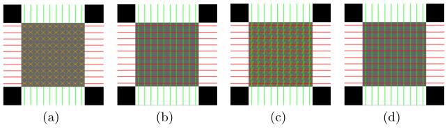
Axial view of the FA of the crossing phantom. Reconstructed fiber directions are shown for (a) CFARI and (b)–(d) the proposed method. The PDs are ground truth directions in (b), ground truth directions with 15° in-plane rotation in (c), and ground truth directions with 15° out-of-plane rotation in (d).

First, we used horizontal and vertical directions as PDs for the horizontal and vertical tracts, respectively. An example of reconstructed directions (for α = 0.5 and β = 0.05) is shown in Fig. 1(b), and is compared with CFARI results in Fig. 1(a). The standard color scheme in DTI is used. Directions with small ${\tilde{f}}_{n_i}$’s are interpreted as components of isotropic diffusion; therefore we only show directions with ${\tilde{f}}_{n_i}>0.1$. It can be seen that in crossing regions, CFARI fails to produce the correct configuration while the proposed method successfully generates the correct crossing pattern.

Next, we studied the effect of inaccurate PDs. To introduce errors in the PDs, we rotated the true directions by θ = 15° to obtain PDs. We tested two cases of rotations: in and out of the axial plane. Specifically, in the first case, the horizontal and vertical directions are both clockwise rotated in the axial plane; and in the second case, the horizontal directions are rotated around the vertical line out of the axial plane and the vertical directions are rotated around the horizontal line out of the axial plane. The results are shown in Figs. 1(c) and 1(d) for the two cases, respectively. In both cases, the proposed method correctly reconstructs noncrossing fiber directions. For the PDs with in-plane rotation, the proposed method is still able to find the crossing directions, although it also produces incorrect fiber directions. For the PDs with out-of-plane rotation, the proposed method successfully reconstructs the crossing directions.

To make the simulation more realistic, besides the noise-free phantom test, Rician noise (σ = 0.06) was also added to the digital phantom. And we tested with different values of and . To quantitatively evaluate the results, we define two error measures:

$$e_1=\frac{1}{N_1}\sum _{\underset{\tilde{f}{n}_i>t}{i=1}}^5\underset{j}{\min }\arccos ({\mathit{v}}_{n_i}\cdot {\mathit{u}}_j)\cdot \frac{180°}{\pi }$$ (12)

$$e_2=\frac{1}{N_2}\sum _{j=1}^{N_2}\underset{i:{\tilde{f}}_{n_i}>t}{\min }\arccos ({\mathit{v}}_{n_i}\cdot {\mathit{u}}_j)\cdot \frac{180°}{\pi }.$$ (13)

Here N₁ is the number of directions with normalized mixture fractions ${\tilde{f}}_{n_i}$ larger than a threshold t (in this case t = 0.1), v_ni is the reconstructed fiber direction, and N₂ is the number of ground truth crossing directions u_j. N₂ can be 1 or 2, depending on whether fiber crossing exists at the location. e₁ measures if the reconstructed directions are away from the ground truth, and e₂ measures if each true direction is properly reconstructed. Note that using only e₁ or e₂ is insufficient because the reconstructed directions can agree well with one of the true crossing directions and ignore the other, or each true direction is properly reconstructed but there are other incorrect reconstructed directions.

The average errors in the noncrossing and crossing regions are plotted in Figs. 2 to 5. Here we used the true fiber directions and their 15° rotated versions as PDs. For the rotated directions, the results in the in-plane and out-of-plane cases are averaged. Note that α = 0 is equivalent to CFARI results.

Fig. 2.

Average e₁ errors in noncrossing regions with different noise level σ, PD inaccuracy θ, and the parameters of α and β.

Fig. 5.

Average e₂ errors in crossing regions with different noise level σ, PD inaccuracy θ, and the parameters of α and β.

In noncrossing regions, from Figs. 2 and 3, it can be seen that when errors are introduced in the PDs, the correct fiber directions can still be obtained with proper weighting of prior knowledge. For example, as shown in Figs. 2(b) and 3(b), α = 0.3 and β = 0.6 give zero e₁ and e₂ errors. When noise is added, the use of ground truth as PDs leads to more accurate estimation, as shown in Figs. 2(c) and 3(c). When an error of 15° is introduced, the proposed method can still reduce the effect of noise with proper α and β (see α = 0.5 and β = 0.6 in Figs. 2(d) and 3(d)).

Fig. 3.

Average e₂ errors in noncrossing regions with different noise level σ, PD inaccuracy θ, and the parameters of α and β.

In crossing regions, the use of ground truth as PDs produces correct crossing directions in both the noise-free and the noisy cases (see Figs. 4(a), 4(c), 5(a) and 5(c)). When errors are introduced in the PDs, in both the noise-free and the noisy cases, it is still possible to obtain crossing directions that are close to truth with proper α and β (for example, α = 0.6 and β = 0.05 in Figs. 4(b) and 5(b), and α = 0.5 and β = 1.0 in Figs. 4(d) and 5(d)). Note that in the crossing regions, CFARI, represented by α = 0, cannot find the correct crossing directions. In these examples, the errors of the proposed method can be smaller than the errors introduced in the PDs, which indicates that the proposed result is a better estimate than simply using the prior directions as the estimate.

Fig. 4.

Average e₁ errors in crossing regions with different noise level σ, PD inaccuracy θ, and the parameters of α and β.

3.2 In Vivo Tongue Diffusion Data

Next, we applied our method to in vivo tongue diffusion data of a control subject. Diffusion weighted images were acquired on a 3T MR scanner (Magnetom Trio, Siemens Medical Solutions, Erlangen, Germany) in about two minutes and 30 seconds. Each scan has 12 gradient directions and one b0 image. The b-value is 500 s/mm². The field of view (FOV) is 240 mm × 240 mm × 84 mm. The resolution is 3 mm isotropic.

To obtain PDs, we built a template by manually identifying regions of interest (ROIs) for the genioglossus (GG), the transverse muscle (T), and the vertical muscle (V) on a high resolution structural image (0.8 mm isotropic) of a subject according to [15]. T interdigitates with GG near the mid-sagittal planes and with V on lateral parts of the tongue. The b0 image was also acquired for this template subject in the space of the structural image. The ROIs were then subsampled to have the same resolution with the b0 image. Using SyN registration [2] between b0 images with mutual information as the similarity metric, the template was deformed to the test subject.

Based on the deformed ROIs of GG, T, and V, PDs can be determined. GG and V are known to be fan-shaped; therefore, to calculate the PDs at each voxel (x_i, y_i, z_i) belonging to GG or V, we manually identified the origin point (x₀, y₀, z₀) of GG in the mid-sagittal slice only. Then the PD for GG or V is w_GG/V = (0, y_i − y₀, z_i − z₀). Since T propagates transversely, we use w_T = (1, 0, 0) as the PDs for T. An example of the PDs on the test subject is shown in Fig. 6(a). Note that in the sagittal view, left-right directions are not shown.

Fig. 6.

Fiber directions. Results are compared between the proposed method and CFARI in (b) and (c) in the highlighted regions in (a).

The proposed method was then performed with the PDs. We fixed β = 1 and tested with different α’s. The result is compared with CFARI in Figs. 6(b) and 6(c). We focus on the highlighted areas in Fig. 6(a). Only directions with normalized mixture fractions ${\tilde{f}}_{n_i}>0.1$ are shown. In Fig. 6(b), CFARI does not generate a good fanning pattern for GG, while by tuning α our method is able to reconstruct the fan-shaped directions. Also, in Fig. 6(c), CFARI does not produce the transverse fiber directions while in the proposed method, as α increases, transverse patterns become more obvious.

We then applied fiber tracking with the CFARI results and the proposed results (for α = 0.5 and β = 1). We implemented a variation of INFACT tracking from [11]. The difference is that in seeding a voxel, all the reconstructed directions are used instead of only the one with the largest mixture. Seeding ROIs are placed in parts of T and GG near the mid-sagittal plane, and the results are shown in Fig. 7. Each fiber segment is color-coded by the local orientation using the standard DTI color scheme. Compared to CFARI, the proposed method reconstructs many more transverse fibers and produces a smoother fan-shaped GG.

Fig. 7.

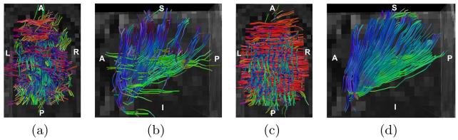
Fiber tracking results: CFARI results seeded in (a) T and (b) GG; proposed results seeded in (c) T and (d) GG. T is viewed from above and GG is viewed from the left.

4 Discussion

To recover crossing fiber directions, more advanced diffusion imaging, such as high angular resolution diffusion imaging (HARDI) [16] and diffusion spectrum imaging [17] (DSI), have been developed. Since HARDI and DSI usually require long acquisition time, which limits their use in clinical research, efforts have also been made to accelerate the imaging process [5]. For example, [5] reduces the scan time from 50 minutes to 17 minutes. However, in the application of tongue diffusion imaging, even accelerated imaging currently may not satisfy the scan time of around 2.5 minutes.

Like [13] and [11], we do not explicitly enforce the constraint of ||f||₁ = 1. As discussed in [7], the general sparse reconstruction problem (without prior knowledge) should be formulated as

$$\widehat{\mathit{f}}=\underset{\mathit{f}\ge 0,{\mid \mid \mathit{f}\mid \mid }_1=1}{\arg \min }{\mid \mid \mathbf{G}\mathit{f}-\mathit{y}\mid \mid }_2^2+\beta {\mid \mid \mathit{f}\mid \mid }_0.$$ (14)

The CFARI algorithm [11] can be viewed as first relaxing the constraint ||f|| = 1, then approximating the ℓ₀-norm with the ℓ₁-norm, and finally reprojecting f onto the plane ||f||₁ = 1. As shown in [11], the approximation is able to resolve crossing fibers. The proposed work further generalizes the approximation with weighted ℓ₁-norm using a Bayesian framework, where prior directional information is incorporated. As demonstrated in the results, the generalization can better distinguish interdigitated tongue muscles with limited gradient directions.

We have assumed a Rician noise model and approximated it with a Gaussian model. It should be noted that in the case of parallel imaging, the noise can follow a noncentral χ distribution [8]. However, in our application, the Gaussian model provides a reasonable approximation in practice.

The PDs are calculated based on the deformed muscle ROIs. An alternative way of calculation is deforming the PDs drawn on the template to the target with the deformation field. As well as the spatial position, the orientation of the PDs should also be rotated according to the deformation field, as suggested in [1]. However, we discovered that although deformable registration can provide a general location of the tracts, due to the low contrast of b0 images, the detailed local deformation is not necessarily accurate, leading to distorted PDs. Therefore, we choose to calculate the PDs as proposed.

The proposed method relies on the ability of specifying PDs. Because of the well organized structures of the tongue muscles, the PDs are achievable for normal subjects. When applied to patients with glossectomy, the current prior knowledge in the lesion may be misleading. Thus, a criterion for using the PDs should be decided or the PDs for patients can be determined in a different way.

Currently, the choice of α and β is empirically fixed for all the voxels. However, the weight of sparsity and prior knowledge can depend on the signal-to-noise ratio (SNR). An improvement could be to determine adaptive α and β based on the estimation of SNR. For example, the SNR can be roughly estimated using image intensities of background and foreground voxels.

5 Conclusion

We have introduced a Bayesian formulation to introduce prior knowledge into a multi-tensor estimation framework. It is particularly suited for situations where acquisitions must be fast such as in in vivo tongue imaging. We use a MAP framework, where prior directional knowledge and sparsity are incorporated in the prior distribution and data fidelity is ensured in the likelihood term. The problem is solved as a noise-aware version of a weighted ℓ₁-norm minimization. Experiments on a digital phantom and in vivo tongue diffusion data demonstrate that the proposed method can reconstruct crossing directions with limited diffusion weighted imaging.

References

- 1.Alexander DC, Pierpaoli C, Basser PJ, Gee JC. Spatial transformations of diffusion tensor magnetic resonance images. Medical Imaging, IEEE Transactions on. 2001;20(11):1131–1139. doi: 10.1109/42.963816. [DOI] [PubMed] [Google Scholar]
- 2.Avants BB, Epstein CL, Grossman M, Gee JC. Symmetric diffeomorphic image registration with cross-correlation: evaluating automated labeling of elderly and neurodegenerative brain. Medical Image Analysis. 2008;12(1):26–41. doi: 10.1016/j.media.2007.06.004. [DOI] [PMC free article] [PubMed] [Google Scholar]
- 3.Basser PJ, Mattiello J, LeBihan D. MR diffusion tensor spectroscopy and imaging. Biophysical Journal. 1994;66(1):259–267. doi: 10.1016/S0006-3495(94)80775-1. [DOI] [PMC free article] [PubMed] [Google Scholar]
- 4.Behrens TEJ, Berg HJ, Jbabdi S, Rushworth MFS, Woolrich MW. Probabilistic diffusion tractography with multiple fibre orientations: What can we gain? NeuroImage. 2007;34(1):144–155. doi: 10.1016/j.neuroimage.2006.09.018. [DOI] [PMC free article] [PubMed] [Google Scholar]
- 5.Bilgic B, Setsompop K, Cohen-Adad J, Yendiki A, Wald LL, Adalsteinsson E. Accelerated diffusion spectrum imaging with compressed sensing using adaptive dictionaries. Magnetic Resonance in Medicine. 2012;68(6):1747–1754. doi: 10.1002/mrm.24505. [DOI] [PMC free article] [PubMed] [Google Scholar]
- 6.Candes EJ, Wakin MB, Boyd SP. Enhancing sparsity by reweighted ℓ1 minimization. Journal of Fourier Analysis and Applications. 2008;14(5-6):877–905. [Google Scholar]
- 7.Daducci A, Van De Ville D, Thiran JP, Wiaux Y. Reweighted sparse deconvolution for high angular resolution diffusion MRI. 2012. arXiv preprint arXiv:1208.2247. [Google Scholar]
- 8.Dietrich O, Raya JG, Reeder SB, Ingrisch M, Reiser MF, Schoenberg SO. Influence of multichannel combination, parallel imaging and other reconstruction techniques on MRI noise characteristics. Magnetic Resonance Imaging. 2008;26(6):754–762. doi: 10.1016/j.mri.2008.02.001. [DOI] [PubMed] [Google Scholar]
- 9.Gudbjartsson H, Patz S. The Rician distribution of noisy MRI data. Magnetic Resonance in Medicine. 1995;34(6):910–914. doi: 10.1002/mrm.1910340618. [DOI] [PMC free article] [PubMed] [Google Scholar]
- 10.Kim SJ, Koh K, Lustig M, Boyd S. An efficient method for compressed sensing. Image Processing; IEEE International Conference on; 2007; pp. III–117. ICIP 2007. IEEE (2007) [Google Scholar]
- 11.Landman BA, Bogovic JA, Wan H, ElShahaby FEZ, Bazin PL, Prince JL. Resolution of crossing fibers with constrained compressed sensing using diffusion tensor MRI. NeuroImage. 2012;59(3):2175–2186. doi: 10.1016/j.neuroimage.2011.10.011. [DOI] [PMC free article] [PubMed] [Google Scholar]
- 12.Peled S, Friman O, Jolesz F, Westin CF. Geometrically constrained two-tensor model for crossing tracts in DWI. Magnetic Resonance Imaging. 2006;24(9):1263–1270. doi: 10.1016/j.mri.2006.07.009. [DOI] [PMC free article] [PubMed] [Google Scholar]
- 13.Ramirez-Manzanares A, Rivera M, Vemuri BC, Carney P, Mareci T. Diffusion basis functions decomposition for estimating white matter intravoxel fiber geometry. Medical Imaging, IEEE Transactions on. 2007;26(8):1091–1102. doi: 10.1109/TMI.2007.900461. [DOI] [PubMed] [Google Scholar]
- 14.Stejskal EO, Tanner JE. Spin diffusion measurements: spin echoes in the presence of a time-dependent field gradient. The Journal of Chemical Physics. 1965;42(1):288. [Google Scholar]
- 15.Takemoto H. Morphological analyses of the human tongue musculature for three-dimensional modeling. Journal of Speech, Language, and Hearing Research. 2001;44(1):95–107. doi: 10.1044/1092-4388(2001/009). [DOI] [PubMed] [Google Scholar]
- 16.Tuch DS, Reese TG, Wiegell MR, Makris N, Belliveau JW, Wedeen VJ. High angular resolution diffusion imaging reveals intravoxel white matter fiber heterogeneity. Magnetic Resonance in Medicine. 2002;48(4):577–582. doi: 10.1002/mrm.10268. [DOI] [PubMed] [Google Scholar]
- 17.Wedeen VJ, Hagmann P, Tseng WYI, Reese TG, Weissko RM. Mapping complex tissue architecture with diffusion spectrum magnetic resonance imaging. Magnetic Resonance in Medicine. 2005;54(6):1377–1386. doi: 10.1002/mrm.20642. [DOI] [PubMed] [Google Scholar]