Learning Graphical Models With Hubs

Abstract

We consider the problem of learning a high-dimensional graphical model in which there are a few hub nodes that are densely-connected to many other nodes. Many authors have studied the use of an ℓ₁ penalty in order to learn a sparse graph in the high-dimensional setting. However, the ℓ₁ penalty implicitly assumes that each edge is equally likely and independent of all other edges. We propose a general framework to accommodate more realistic networks with hub nodes, using a convex formulation that involves a row-column overlap norm penalty. We apply this general framework to three widely-used probabilistic graphical models: the Gaussian graphical model, the covariance graph model, and the binary Ising model. An alternating direction method of multipliers algorithm is used to solve the corresponding convex optimization problems. On synthetic data, we demonstrate that our proposed framework outperforms competitors that do not explicitly model hub nodes. We illustrate our proposal on a webpage data set and a gene expression data set.

1. Introduction

Graphical models are used to model a wide variety of systems, such as gene regulatory networks and social interaction networks. A graph consists of a set of p nodes, each representing a variable, and a set of edges between pairs of nodes. The presence of an edge between two nodes indicates a relationship between the two variables. In this manuscript, we consider two types of graphs: conditional independence graphs and marginal independence graphs. In a conditional independence graph, an edge connects a pair of variables if and only if they are conditionally dependent—dependent conditional upon the other variables. In a marginal independence graph, two nodes are joined by an edge if and only if they are marginally dependent—dependent without conditioning on the other variables.

In recent years, many authors have studied the problem of learning a graphical model in the high-dimensional setting, in which the number of variables p is larger than the number of observations n. Let X be a n × p matrix, with rows x₁, …, x_n. Throughout the rest of the text, we will focus on three specific types of graphical models:

1. A Gaussian graphical model, where ${\mathbf{x}}_1,\dots ,{\mathbf{x}}_n\stackrel{\mathrm{i}.\mathrm{i}.\mathrm{d}.}{~}N(\mathbf{0},\mathbf{\sum })$. In this setting, (Σ⁻¹)_jj′ = 0 for some j ≠ j′ if and only if the jth and j′th variables are conditionally independent (Mardia et al., 1979); therefore, the sparsity pattern of Σ⁻¹ determines the conditional independence graph.

2. A Gaussian covariance graph model, where ${\mathbf{x}}_1,\dots ,{\mathbf{x}}_n\stackrel{\mathrm{i}.\mathrm{i}.\mathrm{d}.}{~}N(\mathbf{0},\mathbf{\sum })$. Then Σ_jj′ = 0 for some j ≠ j′ if and only if the jth and j′th variables are marginally independent. Therefore, the sparsity pattern of Σ determines the marginal independence graph.

3. A binary Ising graphical model, where x₁,…,x_n are i.i.d. with density function

   $$p\left(\mathbf{x},\mathbf{\Theta }\right)=\frac{1}{Z(\mathbf{\Theta })}\exp \left[\sum _{j=1}^p{\theta }_{\mathit{jj}}{x}_j+\sum _{1\le j<j^{\prime }\le p}{\theta }_{j{j}^{\prime }}{x}_j{x}_{j^{\prime }}\right],$$

   where Θ is a p × p symmetric matrix, and Z(Θ) is the partition function, which ensures that the density sums to one. Here, x is a binary vector, and θ_jj′ = 0 if and only if the jth and j′th variables are conditionally independent. The sparsity pattern of Θ determines the conditional independence graph.

To construct an interpretable graph when p > n, many authors have proposed applying an ℓ₁ penalty to the parameter encoding each edge, in order to encourage sparsity. For instance, such an approach is taken by Yuan and Lin (2007a), Friedman et al. (2007), Rothman et al. (2008), and Yuan (2008) in the Gaussian graphical model; El Karoui (2008), Bickel and Levina (2008), Rothman et al. (2009), Bien and Tibshirani (2011), Cai and Liu (2011), and Xue et al. (2012) in the covariance graph model; and Lee et al. (2007), Höfling and Tibshirani (2009), and Ravikumar et al. (2010) in the binary model.

However, applying an ℓ₁ penalty to each edge can be interpreted as placing an independent double-exponential prior on each edge. Consequently, such an approach implicitly assumes that each edge is equally likely and independent of all other edges; this corresponds to an Erdős-Rényi graph in which most nodes have approximately the same number of edges (Erdős and Rényi, 1959). This is unrealistic in many real-world networks, in which we believe that certain nodes (which, unfortunately, are not known a priori) have a lot more edges than other nodes. An example is the network of webpages in the World Wide Web, where a relatively small number of webpages are connected to many other webpages (Barabási and Albert, 1999). A number of authors have shown that real-world networks are scale-free, in the sense that the number of edges for each node follows a power-law distribution; examples include gene-regulatory networks, social networks, and networks of collaborations among scientists (among others, Barabási and Albert, 1999; Barabási, 2009; Liljeros et al., 2001; Jeong et al., 2001; Newman, 2000; Li et al., 2005). More recently, Hao et al. (2012) have shown that certain genes, referred to as super hubs, regulate hundreds of downstream genes in a gene regulatory network, resulting in far denser connections than are typically seen in a scale-free network.

In this , we refer to very densely-connected nodes, such as the “super hubs” considered in Hao et al. (2012), as hubs. When we refer to hubs, we have in mind nodes that are connected to a very substantial number of other nodes in the network—and in particular, we are referring to nodes that are much more densely-connected than even the most highly-connected node in a scale-free network. An example of a network containing hub nodes is shown in Figure 1.

Figure 1.

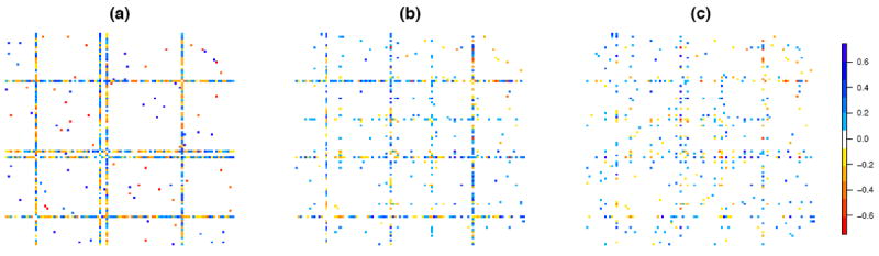
(a): Heatmap of the inverse covariance matrix in a toy example of a Gaussian graphical model with four hub nodes. White elements are zero and colored elements are non-zero in the inverse covariance matrix. Thus, colored elements correspond to edges in the graph. (b): Estimate from the hub graphical lasso, proposed in this paper. (c): Graphical lasso estimate.

Here we propose a convex penalty function for estimating graphs containing hubs. Our formulation simultaneously identifies the hubs and estimates the entire graph. The penalty function yields a convex optimization problem when combined with a convex loss function. We consider the application of this hub penalty function in modeling Gaussian graphical models, covariance graph models, and binary Ising models. Our formulation does not require that we know a priori which nodes in the network are hubs.

In related work, several authors have proposed methods to estimate a scale-free Gaussian graphical model (Liu and Ihler, 2011; Defazio and Caetano, 2012). However, those methods do not model hub nodes—the most highly-connected nodes that arise in a scale-free network are far less connected than the hubs that we consider in our formulation. Under a different framework, some authors proposed a screening-based procedure to identify hub nodes in the context of Gaussian graphical models (Hero and Rajaratnam, 2012; Firouzi and Hero, 2013). Our proposal outperforms such approaches when hub nodes are present (see discussion in Section 3.5.4).

In Figure 1, the performance of our proposed approach is shown in a toy example in the context of a Gaussian graphical model. We see that when the true network contains hub nodes (Figure 1(a)), our proposed approach (Figure 1(b)) is much better able to recover the network than is the graphical lasso (Figure 1(c)), a well-studied approach that applies an ℓ₁ penalty to each edge in the graph (Friedman et al., 2007).

We present the hub penalty function in Section 2. We then apply it to the Gaussian graphical model, the covariance graph model, and the binary Ising model in Sections 3, 4, and 5, respectively. In Section 6, we apply our approach to a webpage data set and a gene expression data set. We close with a discussion in Section 7.

2. The General Formulation

In this section, we present a general framework to accommodate network with hub nodes.

2.1 The Hub Penalty Function

Let X be a n × p data matrix, Θ a p × p symmetric matrix containing the parameters of interest, and ℓ(X, Θ) a loss function (assumed to be convex in Θ). In order to obtain a sparse and interpretable graph estimate, many authors have considered the problem

$$\underset{\mathbf{\Theta }\in \mathit{S}}{\mathrm{minimize}}\{\ell (\mathbf{X},\mathbf{\Theta })+\lambda {\Vert \mathbf{\Theta }-\mathrm{diag}(\mathbf{\Theta })\Vert }_1\},$$ (1)

where λ is a non-negative tuning parameter, S is some set depending on the loss function, and ∥·∥₁ is the sum of the absolute values of the matrix elements. For instance, in the case of a Gaussian graphical model, we could take ℓ(X, Θ) = −log det Θ + trace(SΘ), the negative log-likelihood of the data, where S is the empirical covariance matrix and S is the set of p × p positive definite matrices. The solution to (1) can then be interpreted as an estimate of the inverse covariance matrix. The ℓ₁ penalty in (1) encourages zeros in the solution. But it typically does not yield an estimate that contains hubs.

In order to explicitly model hub nodes in a graph, we wish to replace the ℓ₁ penalty in (1) with a convex penalty that encourages a solution that can be decomposed as Z+V+V^T, where Z is a sparse symmetric matrix, and V is a matrix whose columns are either entirely zero or almost entirely non-zero (see Figure 2). The sparse elements of Z represent edges between non-hub nodes, and the non-zero columns of V correspond to hub nodes. We achieve this goal via the hub penalty function, which takes the form

$$\mathrm{P}(\mathbf{\Theta })=\underset{{\mathbf{V},\mathbf{Z}:\mathbf{\Theta }=\mathbf{V}+\mathbf{V}}^T+\mathbf{Z}}{\min }\left\{{\lambda }_1{\Vert \mathbf{Z}-\mathrm{diag}\left(\mathbf{Z}\right)\Vert }_1+{\lambda }_2{\Vert \mathbf{V}-\mathrm{diag}\left(\mathbf{V}\right)\Vert }_1+{\lambda }_3\sum _{j=1}^p{\Vert {\left(\mathbf{V}-\mathrm{diag}\left(\mathbf{V}\right)\right)}_j\Vert }_q\right\}.$$ (2)

Figure 2.

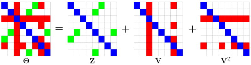
Decomposition of a symmetric matrix Θ into Z + V + V^T, where Z is sparse, and most columns of V are entirely zero. Blue, white, green, and red elements are diagonal, zero, non-zero in Z, and non-zero due to two hubs in V, respectively.

Here λ₁, λ₂, and λ₃ are nonnegative tuning parameters. Sparsity in Z is encouraged via the ℓ₁ penalty on its off-diagonal elements, and is controlled by the value of λ₁. The ℓ₁ and ℓ₁/ℓ_q norms on the columns of V induce group sparsity when q = 2 (Yuan and Lin, 2007b; Simon et al., 2013); λ₃ controls the selection of hub nodes, and λ₂ controls the sparsity of each hub node’s connections to other nodes. The convex penalty (2) can be combined with ℓ(X, Θ) to yield the convex optimization problem

$$\begin{array}{ll}\underset{\mathbf{\Theta }\in \mathit{S},\mathbf{V},\mathbf{Z}}{\mathrm{minimize}}& \{\ell \left(\mathbf{X},\mathbf{\Theta }\right)+{\lambda }_1{\Vert \mathbf{Z}-\mathrm{diag}\left(\mathbf{Z}\right)\Vert }_1+{\lambda }_2{\Vert \mathbf{V}-\mathrm{diag}\left(\mathbf{V}\right)\Vert }_1\\ & +{\lambda }_3\sum _{j=1}^p{\Vert {\left(\mathbf{V}-\mathrm{diag}\left(\mathbf{V}\right)\right)}_j\Vert }_q\}\mathrm{subject\; to}\mathbf{\Theta }=\mathbf{V}+{\mathbf{V}}^T+\mathbf{Z},\end{array}$$ (3)

where the set S depends on the loss function ℓ(X, Θ).

Note that when λ₂ → ∞ or λ₃ → ∞, then (3) reduces to (1). In this paper, we take q = 2, which leads to estimation of a network containing dense hub nodes. Other values of q such as q = ∞ are also possible (see, e.g., Mohan et al., 2014). We note that the hub penalty function is closely related to recent work on overlapping group lasso penalties in the context of learning multiple sparse precision matrices (Mohan et al., 2014).

2.2 Algorithm

In order to solve (3) with q = 2, we use an alternating direction method of multipliers (ADMM) algorithm (see, e.g., Eckstein and Bertsekas, 1992; Boyd et al., 2010; Eckstein, 2012). ADMM is an attractive algorithm for this problem, as it allows us to decouple some of the terms in (3) that are difficult to optimize jointly. In order to develop an ADMM algorithm for (3) with guaranteed convergence, we reformulate it as a consensus problem, as in Ma et al. (2013). The convergence of the algorithm to the optimal solution follows from classical results (see, e.g., the review papers Boyd et al., 2010; Eckstein, 2012).

In greater detail, we let B = (Θ, V, Z), B̃ = (Θ̃, Ṽ, Z̃),

$$\begin{array}{l}f(\mathbf{B})=\ell \left(\mathbf{X},\mathbf{\Theta }\right)+{\lambda }_1{\Vert \mathbf{Z}-\mathrm{diag}\left(\mathbf{Z}\right)\Vert }_1+{\lambda }_2{\Vert \mathbf{V}-\mathrm{diag}\left(\mathbf{V}\right)\Vert }_1+{\lambda }_3\sum _{j=1}^p{\Vert \left(\mathbf{V}-\mathrm{diag}\left(\mathbf{V}\right)\right)\Vert }_2,\\ \end{array}$$

and

$$g(\stackrel{\sim }{\mathbf{B}})=\{\begin{array}{ll}0& \mathrm{if}\stackrel{\sim }{\mathbf{\Theta }}=\stackrel{\sim }{\mathbf{V}}+{\stackrel{\sim }{\mathbf{V}}}^T+\stackrel{\sim }{\mathbf{Z}}\\ \infty & \mathrm{otherwise}.\end{array}$$

Then, we can rewrite (3) as

$$\underset{\mathbf{B},\stackrel{\sim }{\mathbf{B}}}{\mathrm{minimize}}\left\{f\left(\mathbf{B}\right)+g(\stackrel{\sim }{\mathbf{B}})\right\}\mathrm{subject\; to}\mathbf{B}=\stackrel{\sim }{\mathbf{B}}.$$ (4)

The scaled augmented Lagrangian for (4) takes the form

$$\begin{array}{lll}L(\mathbf{B},\stackrel{\sim }{\mathbf{B}},\mathbf{W})& =& \ell \left(\mathbf{X},\mathbf{\Theta }\right)+{\lambda }_1{\Vert \mathbf{Z}-\mathrm{diag}\left(\mathbf{Z}\right)\Vert }_1+{\lambda }_2{\Vert \mathbf{V}-\mathrm{diag}\left(\mathbf{V}\right)\Vert }_1\\ & +& {\lambda }_3\sum _{j=1}^p{\Vert {\left(\mathbf{V}-\mathrm{diag}\left(\mathbf{V}\right)\right)}_j\Vert }_2+g(\stackrel{\sim }{\mathbf{B}})+\frac{\rho }{2}{\Vert \mathbf{B}-\stackrel{\sim }{\mathbf{B}}+\mathbf{W}\Vert }_F^2,\end{array}$$

where B and B̃ are the primal variables, and W = (W₁, W₂, W₃) is the dual variable. Note that the scaled augmented Lagrangian can be derived from the usual Lagrangian by adding a quadratic term and completing the square (Boyd et al., 2010).

A general algorithm for solving (3) is provided in Algorithm 1. The derivation is in Appendix A. Note that only the update for Θ (Step 2(a)i) depends on the form of the convex loss function ℓ(X, Θ). In the following sections, we consider special cases of (3) that lead to estimation of Gaussian graphical models, covariance graph models, and binary networks with hub nodes.

Algorithm 1 ADMM Algorithm for Solving (3).

1. Initialize the parameters:

   1. primal variables Θ, V, Z, Θ̃, Ṽ, and Z̃ to the p × p identity matrix.
   2. dual variables W₁, W₂, and W₃ to the p × p zero matrix.
   3. constants ρ > 0 and τ > 0.

2. Iterate until the stopping criterion $\frac{{\Vert {\mathbf{\Theta }}_t-{\mathbf{\Theta }}_{t-1}\Vert }_F^2}{{\Vert {\mathbf{\Theta }}_{t-1}\Vert }_F^2}\le \tau$ is met, where Θ_t is the value of Θ obtained at the tth iteration:

   1. Update Θ, V, Z:

      1. $\mathbf{\Theta }=\underset{\mathbf{\Theta }\in \mathit{S}}{\mathrm{arg\; min}}\left\{\ell (\mathbf{X},\mathbf{\Theta })+\frac{\rho }{2}{\Vert \mathbf{\Theta }-\stackrel{\sim }{\mathbf{\Theta }}+{\mathbf{W}}_1\Vert }_F^2\right\}$.

      2. Z = S(Z̃ − W₃, $\frac{{\lambda }_1}{\rho }$), diag(Z) = diag(Z̃ − W₃). Here S denotes the soft-thresholding operator, applied element-wise to a matrix: S(A_ij, b) = sign(A_ij) max(|A_ij| − b, 0).

      3. C = Ṽ − W₂ − diag(Ṽ − W₂).

      4. ${\mathbf{V}}_j=\max \left(1-\frac{{\lambda }_3}{\rho {\Vert S\left({\mathbf{C}}_j,{\lambda }_2/\rho \right)\Vert }_2},0\right)·S({\mathbf{C}}_j,{\lambda }_2/\rho )$ for j = 1,…, p.

      5. diag(V) = diag(Ṽ − W₂).

   2. Update Θ̃, Ṽ, Z̃:

      1. $\mathbf{\Gamma }=\frac{\rho }{6}\left[(\mathbf{\Theta }+{\mathbf{W}}_1)-(\mathbf{V}+{\mathbf{W}}_2)-{(\mathbf{V}+{\mathbf{W}}_2)}^T-(\mathbf{Z}+{\mathbf{W}}_3)\right]$.

      2. $\stackrel{\sim }{\mathbf{\Theta }}=\mathbf{\Theta }+{\mathbf{W}}_1-\frac{1}{\rho }\mathbf{\Gamma }$; iii. $\stackrel{\sim }{\mathbf{V}}=\frac{1}{\rho }(\mathbf{\Gamma }+{\mathbf{\Gamma }}^T)+\mathbf{V}+{\mathbf{W}}_2$; iv. $\stackrel{\sim }{\mathbf{Z}}=\frac{1}{\rho }\mathbf{\Gamma }+\mathbf{Z}+{\mathbf{W}}_3$.

   3. Update W₁, W₂, W₃:

      1. W₁ = W₁ + Θ − Θ̃; ii. W₂ = W₂ + V − Ṽ; iii. W₃ = W₃ + Z − Z̃.

3. The Hub Graphical Lasso

Assume that ${\mathbf{x}}_1,\dots ,{\mathbf{x}}_n\stackrel{\mathrm{i}.\mathrm{i}.\mathrm{d}.}{~}N(\mathbf{0},\mathbf{\sum })$. The well-known graphical lasso problem (see, e.g., Friedman et al., 2007) takes the form of (1) with ℓ(X, Θ) = − log det Θ + trace(SΘ), and S the empirical covariance matrix of X:

$$\underset{\mathbf{\Theta }\in \mathit{S}}{\mathrm{minimize}}\{-\mathrm{log\; det}\mathbf{\Theta }+\mathrm{trace}(\mathbf{S\Theta })+\lambda \sum _{j\ne j^{\prime }}|{\mathbf{\Theta }}_{j{j}^{\prime }}|\},$$ (5)

where S = {Θ : Θ ≻ 0 and Θ = Θ^T}. The solution to this optimization problem serves as an estimate for Σ⁻¹. We now use the hub penalty function to extend the graphical lasso in order to accommodate hub nodes.

3.1 Formulation and Algorithm

We propose the hub graphical lasso (HGL) optimization problem, which takes the form

$$\underset{\mathbf{\Theta }\in \mathbf{S}}{\mathrm{minimize}}\left\{-\mathrm{log\; det}\mathbf{\Theta }+\mathrm{trace}(\mathbf{S\Theta })+\mathrm{P}\left(\mathbf{\Theta }\right)\right\}.$$ (6)

Again, S = {Θ : Θ ≻ 0 and Θ = Θ^T}. It encourages a solution that contains hub nodes, as well as edges that connect non-hubs (Figure 1). Problem (6) can be solved using Algorithm 1. The update for Θ in Algorithm 1 (Step 2(a)i) can be derived by minimizing

$$-\mathrm{log\; det}\mathbf{\Theta }+\mathrm{trace}\left(\mathbf{S\Theta }\right)+\frac{\rho }{2}{\Vert \mathbf{\Theta }-\stackrel{\sim }{\mathbf{\Theta }}+{\mathbf{W}}_1\Vert }_F^2$$ (7)

with respect to Θ (note that the constraint Θ ∈ S in (6) is treated as an implicit constraint, due to the domain of definition of the log det function). This can be shown to have the solution

$$\mathbf{\Theta }=\frac{1}{2}\mathbf{U}\left(\mathbf{D}+\sqrt{{\mathbf{D}}^2+\frac{4}{\rho }\mathbf{I}}\right){\mathbf{U}}^T,$$

where UDU^T denotes the eigen-decomposition of $\stackrel{\sim }{\mathbf{\Theta }}-{\mathbf{W}}_1-\frac{1}{\rho }\mathbf{S}$.

The complexity of the ADMM algorithm for HGL is O(p³) per iteration; this is the complexity of the eigen-decomposition for updating Θ. We now briefly compare the computational time for the ADMM algorithm for solving (6) to that of an interior point method (using the solver Sedumi called from cvx). On a 1.86 GHz Intel Core 2 Duo machine, the interior point method takes ~ 3 minutes, while ADMM takes only 1 second, on a data set with p = 30. We present a more extensive run time study for the ADMM algorithm for HGL in Appendix E.

3.2 Conditions for HGL Solution to be Block Diagonal

In order to reduce computations for solving the HGL problem, we now present a necessary condition and a sufficient condition for the HGL solution to be block diagonal, subject to some permutation of the rows and columns. The conditions depend only on the tuning parameters λ₁, λ₂, and λ₃. These conditions build upon similar results in the context of Gaussian graphical models from the recent literature (see, e.g., Witten et al., 2011; Mazumder and Hastie, 2012; Yang et al., 2012b; Danaher et al., 2014; Mohan et al., 2014). Let C₁, C₂, …, C_K denote a partition of the p features.

Theorem 1

A sufficient condition for the HGL solution to be block diagonal with blocks given by C₁, C₂, …, C_K is that $\min \left\{{\lambda }_1,\frac{{\lambda }_2}{2}\right\}>|S_{j{j}^{\prime }}|$ for all j ∈ C_k, j′ ∈ C_k′, k ≠ k′.

Theorem 2

A necessary condition for the HGL solution to be block diagonal with blocks given by C₁, C₂, …, C_K is that $\min \left\{{\lambda }_1,\frac{{\lambda }_2+{\lambda }_3}{2}\right\}>|S_{j{j}^{\prime }}|$ for all j ∈ C_k, j′ ∈ C_k′, k ≠ k′.

Theorem 1 implies that one can screen the empirical covariance matrix S to check if the HGL solution is block diagonal (using standard algorithms for identifying the connected components of an undirected graph; see, e.g., Tarjan, 1972). Suppose that the HGL solution is block diagonal with K blocks, containing p₁, …, p_K features, and ${\sum }_{k=1}^K{p}_k=p$. Then, one can simply solve the HGL problem on the features within each block separately. Recall that the bottleneck of the HGL algorithm is the eigen-decomposition for updating Θ. The block diagonal condition leads to massive computational speed-ups for implementing the HGL algorithm: instead of computing an eigen-decomposition for a p × p matrix in each iteration of the HGL algorithm, we compute the eigen-decomposition of K matrices of dimensions p₁ × p₁, …, p_K × p_K. The computational complexity per-iteration is reduced from O(p³) to ${\sum }_{k=1}^{K}O\left(p_k^3\right)$.

We illustrate the reduction in computational time due to these results in an example with p = 500. Without exploiting Theorem 1, the ADMM algorithm for HGL (with a particular value of λ) takes 159 seconds; in contrast, it takes only 22 seconds when Theorem 1 is applied. The estimated precision matrix has 107 connected components, the largest of which contains 212 nodes.

3.3 Some Properties of HGL

We now present several properties of the HGL optimization problem (6), which can be used to provide guidance on the suitable range for the tuning parameters λ₁, λ₂, and λ₃. In what follows, Z* and V* denote the optimal solutions for Z and V in (6). Let $\frac{1}{s}+\frac{1}{q}=1$ (recall that q appears in Equation 2).

Lemma 3

A sufficient condition for Z* to be a diagonal matrix is that ${\lambda }_1>\frac{{\lambda }_2+{\lambda }_3}{2}$.

Lemma 4

A sufficient condition for V* to be a diagonal matrix is that ${\lambda }_1<\frac{{\lambda }_2}{2}+\frac{{\lambda }_3}{2{\left(p-1\right)}^{1/s}}$.

Corollary 5

A necessary condition for both V* and Z* to be non-diagonal matrices is that $\frac{{\lambda }_2}{2}+\frac{{\lambda }_3}{2{\left(p-1\right)}^{1/s}}\le {\lambda }_1\le \frac{{\lambda }_2+{\lambda }_3}{2}$.

Furthermore, (6) reduces to the graphical lasso problem (5) under a simple condition.

Lemma 6

If q = 1, then (6) reduces to (5) with tuning parameter $\min \left\{{\lambda }_1,\frac{{\lambda }_2+{\lambda }_3}{2}\right\}$.

Note also that when λ₂ → ∞ or λ₃ → ∞, (6) reduces to (5) with tuning parameter λ₁. However, throughout the rest of this paper, we assume that q = 2, and λ₂ and λ₃ are finite.

The solution Θ̂ of (6) is unique, since (6) is a strictly convex problem. We now consider the question of whether the decomposition Θ̂ = V̂ + V̂^T + Ẑ is unique. We see that the decomposition is unique in a certain regime of the tuning parameters. For instance, according to Lemma 3, when ${\lambda }_1>\frac{{\lambda }_2+{\lambda }_3}{2}$, Ẑ is a diagonal matrix and hence V̂ is unique. Similarly, according to Lemma 4, when ${\lambda }_1<\frac{{\lambda }_2}{2}+\frac{{\lambda }_3}{2{\left(p-1\right)}^{1/s}}$, V̂ is a diagonal matrix and hence Ẑ is unique. Studying more general conditions on S and on λ₁, λ₂, and λ₃ such that the decomposition is guaranteed to be unique is a challenging problem and is outside of the scope of this paper.

3.4 Tuning Parameter Selection

In this section, we propose a Bayesian information criterion (BIC)-type quantity for tuning parameter selection in (6). Recall from Section 2 that the hub penalty function (2) decomposes the parameter of interest into the sum of three matrices, Θ = Z + V + V^T, and places an ℓ₁ penalty on Z, and an ℓ₁/ℓ₂ penalty on V.

For the graphical lasso problem in (5), many authors have proposed to select the tuning parameter λ such that Θ̂ minimizes the following quantity:

$$-n·\mathrm{log\; det}(\widehat{\mathbf{\Theta }})+n·\mathrm{trace}(\mathbf{S}\widehat{\mathbf{\Theta }})+\log (n)·|\widehat{\mathbf{\Theta }}|,$$

where |Θ̂| is the cardinality of Θ̂, that is, the number of unique non-zeros in Θ̂ (see, e.g., Yuan and Lin, 2007a).¹

Using a similar idea, we propose the following BIC-type quantity for selecting the set of tuning parameters (λ₁, λ₂,λ₃) for (6):

$$\mathrm{BIC}(\widehat{\mathbf{\Theta }},\widehat{\mathbf{V}},\widehat{\mathbf{Z}})=-n·\mathrm{log\; det}(\widehat{\mathbf{\Theta }})+n·\mathrm{trace}(\mathbf{S}\widehat{\mathbf{\Theta }})+\log (n)·|\widehat{\mathbf{Z}}|+\log (n)·\left(\nu +c·[|\widehat{\mathbf{V}}|-\nu ]\right),$$

where ν is the number of estimated hub nodes, that is, $\nu ={\sum }_{j=1}^p{1}_{\{{\Vert {\widehat{\mathbf{V}}}_j\Vert }_0>0\}}$, c is a constant between zero and one, and |Ẑ| and |V̂| are the cardinalities (the number of unique nonzeros) of Ẑ and V̂, respectively.² We select the set of tuning parameters (λ₁,λ₂, λ₃) for which the quantity BIC(Θ̂, V̂, Ẑ) is minimized. Note that when the constant c is small, BIC(Θ̂, V̂, Ẑ) will favor more hub nodes in V̂. In this manuscript, we take c = 0.2.

3.5 Simulation Study

In this section, we compare HGL to two sets of proposals: proposals that learn an Erdős-Rényi Gaussian graphical model, and proposals that learn a Gaussian graphical model in which some nodes are highly-connected.

3.5.1 Notation and Measures of Performance

We start by defining some notation. Let Θ̂ be the estimate of Θ = Σ⁻¹ from a given proposal, and let Θ̂_j be its jth column. Let H denote the set of indices of the hub nodes in Θ (that is, this is the set of true hub nodes in the graph), and let |H| denote the cardinality of the set. In addition, let Ĥ_r be the set of estimated hub nodes: the set of nodes in Θ̂ that are among the |H| most highly-connected nodes, and that have at least r edges. The values chosen for |H| and r depend on the simulation set-up, and will be specified in each simulation study.

We now define several measures of performance that will be used to evaluate the various methods.

• Number of correctly estimated edges: ${\sum }_{j<j^{\prime }}\left(1_{\{|{\widehat{\mathrm{\Theta }}}_{j{j}^{\prime }}|>{10}^{-5}\mathrm{and}|{\mathrm{\Theta }}_{j{j}^{\prime }}|\ne 0\}}\right)$.

• Proportion of correctly estimated hub edges:

  $$\frac{{\sum }_{j\in H,j\prime \ne j}\left(1_{\{|{\widehat{\mathrm{\Theta }}}_{j{j}^{\prime }}|>{10}^{-5}\mathrm{and}|{\mathrm{\Theta }}_{j{j}^{\prime }}|\ne 0\}}\right)}{{\sum }_{j\in H,j^{\prime }\ne j}\left(1_{\{|{\mathrm{\Theta }}_{j{j}^{\prime }}|\ne 0\}}\right)}.$$

• Proportion of correctly estimated hub nodes: $\frac{|{\widehat{H}}_r\cap H|}{|H|}$.

• Sum of squared errors: ${\sum }_{j<j^{\prime }}{\left({\widehat{\mathrm{\Theta }}}_{j{j}^{\prime }}-{\mathrm{\Theta }}_{j{j}^{\prime }}\right)}^2$.

3.5.2 Data Generation

We consider three set-ups for generating a p × p adjacency matrix A.

1. Network with hub nodes: for all i < j, we set A_ij = 1 with probability 0.02, and zero otherwise. We then set A_ji equal to A_ij. Next, we randomly select |H| hub nodes and set the elements of the corresponding rows and columns of A to equal one with probability 0.7 and zero otherwise.

2. Network with two connected components and hub nodes: the adjacency matrix is generated as $\mathbf{A}=\left(\begin{array}{cc}{\mathbf{A}}_1& 0\\ 0& {\mathbf{A}}_2\end{array}\right)$, with A₁ and A₂ as in Set-up I, each with |H|/2 hub nodes.

3. Scale-free network:³ the probability that a given node has k edges is proportional to k^−α. Barabási and Albert (1999) observed that many real-world networks have α ∈ [2.1, 4]; we took α = 2.5. Note that there is no natural notion of hub nodes in a scale-free network. While some nodes in a scale-free network have more edges than one would expect in an Erdős-Rényi graph, there is no clear distinction between “hub” and “non-hub“ nodes, unlike in Set-ups I and II. In our simulation settings, we consider any node that is connected to more than 5% of all other nodes to be a hub node.⁴

We then use the adjacency matrix A to create a matrix E, as

$$E_{\mathit{ij}}\underset{~}{\mathrm{i}.\mathrm{i}.\mathrm{d}.}\{\begin{array}{ll}0& \mathrm{if}{A}_{\mathit{ij}}=0\\ \mathrm{Unif}([-0.75,-0.25]\cup [0.25,0.75])& \mathrm{otherwise},\end{array}$$

and set $\overline{\mathbf{E}}=\frac{1}{2}(\mathbf{E}+{\mathbf{E}}^T)$. Given the matrix Ē, we set Σ⁻¹ equal to Ē + (0.1 − Λ_min(Ē))I, where Λ_min(Ē) is the smallest eigenvalue of Ē. We generate the data matrix X according to ${\mathbf{x}}_1,\dots ,{\mathbf{x}}_n\stackrel{\mathrm{i}.\mathrm{i}.\mathrm{d}.}{~}N(\mathbf{0},\mathbf{\sum })$. Then, variables are standardized to have standard deviation one.

3.5.3 Comparison to Graphical Lasso and Neighbourhood Selection

In this subsection, we compare the performance of HGL to two proposals that learn a sparse Gaussian graphical model.

• The graphical lasso (5), implemented using the R package glasso.

• The neighborhood selection approach of Meinshausen and Bühlmann (2006), implemented using the R package glasso. This approach involves performing p ℓ₁-penalized regression problems, each of which involves regressing one feature onto the others.

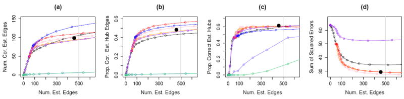
We consider the three simulation set-ups described in the previous section with n = 1000, p = 1500, and |H| = 30 hub nodes in Set-ups I and II. Figure 3 displays the results, averaged over 100 simulated data sets. Note that the sum of squared errors is not computed for Meinshausen and Bühlmann (2006), since it does not directly yield an estimate of Θ = Σ⁻¹.

Figure 3.

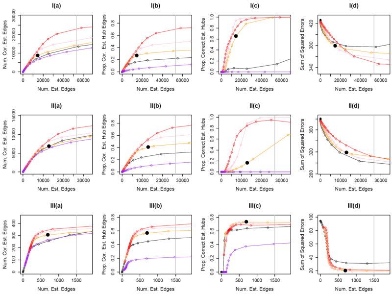
Simulation for Gaussian graphical model. Row I: Results for Set-up I. Row II: Results for Set-up II. Row III: Results for Set-up III. The results are for n = 1000 and p = 1500. In each panel, the x-axis displays the number of estimated edges, and the vertical gray line is the number of edges in the true network. The y-axes are as follows: Column (a): Number of correctly estimated edges; Column (b): Proportion of correctly estimated hub edges; Column (c): Proportion of correctly estimated hub nodes; Column (d): Sum of squared errors. The black solid circles are the results for HGL based on tuning parameters selected using the BIC-type criterion defined in Section 3.4. Colored lines correspond to the graphical lasso (Friedman et al., 2007) ( ); HGL with λ₃ = 0:5 ( ), λ₃ = 1 ( ), and λ₃ = 2 ( ); neighborhood selection (Meinshausen and Bühlmann, 2006) ( ).

HGL has three tuning parameters. To obtain the curves shown in Figure 3, we fixed λ₁ = 0.4, considered three values of λ₃ (each shown in a different color in Figure 3), and used a fine grid of values of λ₂. The solid black circle in Figure 3 corresponds to the set of tuning parameters (λ₁, λ₂, λ₃) for which the BIC as defined in Section 3.4 is minimized. The graphical lasso and Meinshausen and Bühlmann (2006) each involves one tuning parameter; we applied them using a fine grid of the tuning parameter to obtain the curves shown in Figure 3.

Results for Set-up I are displayed in Figures 3-I(a) through 3-I(d), where we calculate the proportion of correctly estimated hub nodes as defined in Section 3.5.1 with r = 300. Since this simulation set-up exactly matches the assumptions of HGL, it is not surprising that HGL outperforms the other methods. In particular, HGL is able to identify most of the hub nodes when the number of estimated edges is approximately equal to the true number of edges. We see similar results for Set-up II in Figures 3-II(a) through 3-II(d), where the proportion of correctly estimated hub nodes is as defined in Section 3.5.1 with r = 150.

In Set-up III, recall that we define a node that is connected to at least 5% of all nodes to be a hub. The proportion of correctly estimated hub nodes is then as defined in Section 3.5.1 with r = 0.05 × p. The results are presented in Figures 3-III(a) through 3-III(d). In this set-up, only approximately three of the nodes (on average) have more than 50 edges, and the hub nodes are not as highly-connected as in Set-up I or Set-up II. Nonetheless, HGL outperforms the graphical lasso and Meinshausen and Bühlmann (2006).

Finally, we see from Figure 3 that the set of tuning parameters (λ₁, λ₂, λ₃) selected using BIC performs reasonably well. In particular, the graphical lasso solution always has BIC larger than HGL, and hence, is not selected.

3.5.4 Comparison to Additional Proposals

In this subsection, we compare the performance of HGL to three additional proposals:

• The partial correlation screening procedure of Hero and Rajaratnam (2012). The elements of the partial correlation matrix (computed using a pseudo-inverse when p > n) are thresholded based on their absolute value, and a hub node is declared if the number of nonzero elements in the corresponding column of the thresholded partial correlation matrix is sufficiently large. Note that the purpose of Hero and Rajaratnam (2012) is to screen for hub nodes, rather than to estimate the individual edges in the network.

• The scale-free network estimation procedure of Liu and Ihler (2011). This is the solution to the non-convex optimization problem

  $$\underset{\mathbf{\Theta }\in \mathit{S}}{\mathrm{minimize}}\left\{-\mathrm{log\; det}\mathbf{\Theta }+\mathrm{trace}(\mathbf{S\Theta })+\alpha \sum _{j=1}^p\log ({\Vert {\theta }_{\backslash j}\Vert }_1+{\epsilon }_j)+\sum _{j=1}^p{\beta }_j|{\theta }_{\mathit{jj}}|\right\},$$ (8)

  where θ_\j = {θ_jj′∣j′ ≠ j}, and ε_j, β_j, and α are tuning parameters. Here, S = {Θ: Θ ≻ 0 and Θ = Θ^T}.

• Sparse partial correlation estimation procedure of Peng et al. (2009), implemented using the R package space. This is an extension of the neighborhood selection approach of Meinshausen and Bühlmann (2006) that combines p ℓ₁-penalized regression problems in order to obtain a symmetric estimator. The authors claimed that the proposal performs well in estimating a scale-free network.

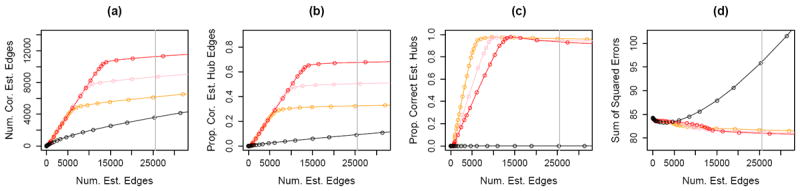
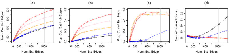
We generated data under Set-ups I and III (described in Section 3.5.2) with n = 250 and p = 500,⁵ and with |H| = 10 for Set-up I. The results, averaged over 100 data sets, are displayed in Figures 4 and 5.

Figure 4.

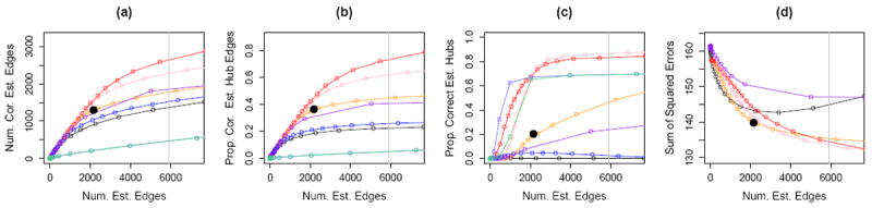
Simulation for the Gaussian graphical model. Set-up I was applied with n = 250 and p = 500. Details of the axis labels and the solid black circles are as in Figure 3. The colored lines correspond to the graphical lasso (Friedman et al., 2007) ( ); HGL with λ₃ = 1 ( ), λ₃ = 2 ( ), and λ₃ = 3 ( ); the hub screening procedure (Hero and Rajaratnam, 2012) with d = 10 ( ) and d = 20 ( ); the scale-free network approach (Liu and Ihler, 2011) ( ); sparse partial correlation estimation (Peng et al., 2009) ( ).

Figure 5.

Simulation for the Gaussian graphical model. Set-up III was applied with n = 250 and p = 500. Details of the axis labels and the solid black circles are as in Figure 3. The colored lines correspond to the graphical lasso (Friedman et al., 2007) ( ); HGL with λ₃ = 1 ( ), λ₃ = 2 ( ), and λ₃ = 3 ( ); the hub screening procedure (Hero and Rajaratnam, 2012) with d = 10 ( ) and d = 20 ( ); the scale-free network approach (Liu and Ihler, 2011) ( ); sparse partial correlation estimation (Peng et al., 2009) ( ).

To obtain Figures 4 and 5, we applied Liu and Ihler (2011) using a fine grid of α values, and using the choices for β_j and ε_j specified by the authors: β_j = 2α/ε_j, where ε_j is a small constant specified in Liu and Ihler (2011). There are two tuning parameters in Hero and Rajaratnam (2012): (1) ρ, the value used to threshold the partial correlation matrix, and (2) d, the number of non-zero elements required for a column of the thresholded matrix to be declared a hub node. We used d = {10,20} in Figures 4 and 5, and used a fine grid of values for ρ. Note that the value of d has no effect on the results for Figures 4(a)-(b) and Figures 5(a)-(b), and that larger values of d tend to yield worse results in Figures 4(c) and 5(c). For Peng et al. (2009), we used a fine grid of tuning parameter values to obtain the curves shown in Figures 4 and 5. The sum of squared errors was not reported for Peng et al. (2009) and Hero and Rajaratnam (2012) since they do not directly yield an estimate of the precision matrix. As a baseline reference, the graphical lasso is included in the comparison.

We see from Figure 4 that HGL outperforms the competitors when the underlying network contains hub nodes. It is not surprising that Liu and Ihler (2011) yields better results than the graphical lasso, since the former approach is implemented via an iterative procedure: in each iteration, the graphical lasso is performed with an updated tuning parameter based on the estimate obtained in the previous iteration. Hero and Rajaratnam (2012) has the worst results in Figures 4(a)-(b); this is not surprising, since the purpose of Hero and Rajaratnam (2012) is to screen for hub nodes, rather than to estimate the individual edges in the network.

From Figure 5, we see that the performance of HGL is comparable to that of Liu and Ihler (2011) and Peng et al. (2009) under the assumption of a scale-free network; note that this is the precise setting for which Liu and Ihler (2011)’s proposal is intended, and Peng et al. (2009) reported that their proposal performs well in this setting. In contrast, HGL is not intended for the scale-free network setting (as mentioned in the Introduction, it is intended for a setting with hub nodes). Again, Liu and Ihler (2011) and Peng et al. (2009) outperform the graphical lasso, and Hero and Rajaratnam (2012) has the worst results in Figures 5(a)-(b). Finally, we see from Figures 4 and 5 that the BIC-type criterion for HGL proposed in Section 3.4 yields good results.

4. The Hub Covariance Graph

In this section, we consider estimation of a covariance matrix under the assumption that ${\mathbf{x}}_1,\dots ,{\mathbf{x}}_n\stackrel{\mathrm{i}.\mathrm{i}.\mathrm{d}.}{~}N(\mathbf{0},\mathbf{\sum })$; this is of interest because the sparsity pattern of Σ specifies the structure of the marginal independence graph (see, e.g., Drton and Richardson, 2003; Chaudhuri et al., 2007; Drton and Richardson, 2008). We extend the covariance estimator of Xue et al. (2012) to accommodate hub nodes.

4.1 Formulation and Algorithm

Xue et al. (2012) proposed to estimate Σ using

$$\widehat{\mathbf{\sum }}=\underset{\mathbf{\sum }\in \mathit{S}}{\mathrm{arg\; min}}\left\{\frac{1}{2}{\Vert \mathbf{\sum }-\mathbf{S}\Vert }_F^2+\lambda {\Vert \mathbf{\sum }\Vert }_1\right\},$$ (9)

where S is the empirical covariance matrix, S = {Σ : Σ ≽ εI and Σ = Σ^T}, and ε is a small positive constant; we take ε = 10⁻⁴. We extend (9) to accommodate hubs by imposing the hub penalty function (2) on Σ. This results in the hub covariance graph (HCG) optimization problem,

$$\underset{\mathbf{\sum }\in \mathit{S}}{\mathrm{minimize}}\left\{\frac{1}{2}{\Vert \mathbf{\sum }-\mathbf{S}\Vert }_F^2+\mathrm{P}(\mathbf{\sum })\right\},$$

which can be solved via Algorithm 1. To update Θ = Σ in Step 2(a)i, we note that

$$\underset{\mathbf{\sum }\in \mathit{S}}{\mathrm{arg\; min}}\left\{\frac{1}{2}{\Vert \mathbf{\sum }-\mathbf{S}\Vert }_F^2+\frac{\rho }{2}{\Vert \mathbf{\sum }-\mathbf{\sum }^{\sim }+{\mathbf{W}}_1\Vert }_F^2\right\}=\frac{1}{1+\rho }{(\mathbf{S}+\rho \mathbf{\sum }^{\sim }-\rho {\mathbf{W}}_1)}^{+},$$

where (A)⁺ is the projection of a matrix A onto the convex cone {Σ ≽ εI}. That is, if ${\sum }_{j=1}^p{d}_j{\mathbf{u}}_j{\mathbf{u}}_j^T$ denotes the eigen-decomposition of the matrix A, then (A)⁺ is defined as ${\sum }_{j=1}^p\max (d_j,\epsilon ){\mathbf{u}}_j{\mathbf{u}}_j^T$. The complexity of the ADMM algorithm is O(p³) per iteration, due to the complexity of the eigen-decomposition for updating Σ.

4.2 Simulation Study

We compare HCG to two competitors for obtaining a sparse estimate of Σ:

1. The non-convex ℓ₁-penalized log-likelihood approach of Bien and Tibshirani (2011), using the R package spcov. This approach solves

   $$\underset{\mathbf{\sum }\succ 0}{\mathrm{minimize}}\{\mathrm{log\; det}\mathbf{\sum }+\mathrm{trace}({\mathbf{\sum }}^{-1}\mathbf{S})+\lambda {\Vert \mathbf{\sum }\Vert }_1\}.$$

2. The convex ℓ₁-penalized approach of Xue et al. (2012), given in (9).

We first generated an adjacency matrix A as in Set-up I in Section 3.5.2, modified to have |H| = 20 hub nodes. Then Ē was generated as described in Section 3.5.2, and we set Σ equal to Ē + (0.1 − Λ_min (Ē))I. Next, we generated. ${\mathbf{x}}_1,\dots ,{\mathbf{x}}_n\stackrel{\mathrm{i}.\mathrm{i}.\mathrm{d}.}{~}N(\mathbf{0},\mathbf{\sum })$. Finally, we standardized the variables to have standard deviation one. In this simulation study, we set n = 500 and p = 1000.

Figure 6 displays the results, averaged over 100 simulated data sets. We calculated the proportion of correctly estimated hub nodes as defined in Section 3.3.1 with r = 200. We used a fine grid of tuning parameters for Xue et al. (2012) in order to obtain the curves shown in each panel of Figure 6. HCG involves three tuning parameters, λ₁, λ₂, and λ₃. We fixed λ₁ = 0.2, considered three values of λ₃ (each shown in a different color), and varied λ₂ in order to obtain the curves shown in Figure 6.

Figure 6.

Covariance graph simulation with n = 500 and p = 1000. Details of the axis labels are as in Figure 3. The colored lines correspond to the proposal of Xue et al. (2012) ( ); HCG with λ₃ = 1 ( ), λ₃ = 1:5 ( ), and λ₃ = 2 ( ).

Figure 6 does not display the results for the proposal of Bien and Tibshirani (2011), due to computational constraints in the spcov R package. Instead, we compared our proposal to that of Bien and Tibshirani (2011) using n = 100 and p = 200; those results are presented in Figure 10 in Appendix D.

We see that HCG outperforms the proposals of Xue et al. (2012) (Figures 6 and 10) and Bien and Tibshirani (2011) (Figure 10). These results are not surprising, since those other methods do not explicitly model the hub nodes.

Figure 10.

Covariance graph simulation with n = 100 and p = 200. Details of the axis labels are as in Figure 3. The colored lines correspond to the proposal of Xue et al. (2012) ( ); HCG with λ₃ = 1 ( ), λ₃ = 1.5 ( ), and λ₃ = 2 ( ); and the proposal of Bien and Tibshirani (2011) ( ).

5. The Hub Binary Network

In this section, we focus on estimating a binary Ising Markov random field, which we refer to as a binary network. We refer the reader to Ravikumar et al. (2010) for an in-depth discussion of this type of graphical model and its applications.

In this set-up, each entry of the n × p data matrix X takes on a value of zero or one. We assume that the observations x₁, …, x_n are i.i.d. with density

$$p(\mathbf{x},\mathbf{\Theta })=\frac{1}{Z(\mathbf{\Theta })}\exp \left[\sum _{j=1}^p{\theta }_{\mathit{jj}}{x}_j+\sum _{1\le j\le j^{\prime }\le p}{\theta }_{j{j}^{\prime }{x}_j{x}_{j^{\prime }}}\right],$$ (10)

where Z(Θ) is the partition function, which ensures that the density sums to one. Here Θ is a p × p symmetric matrix that specifies the network structure: θ_jj′ = 0 implies that the jth and j′th variables are conditionally independent.

In order to obtain a sparse graph, Lee et al. (2007) considered maximizing an ℓ₁-penalized log-likelihood under this model. Due to the difficulty in computing the log-partition function, several authors have considered alternative approaches. For instance, Ravikumar et al. (2010) proposed a neighborhood selection approach. The proposal of Ravikumar et al. (2010) involves solving p logistic regression separately, and hence, the estimated parameter matrix is not symmetric. In contrast, several authors considered maximizing an ℓ₁-penalized pseudo-likelihood with a symmetric constraint on Θ (see, e.g., Höfling and Tibshirani, 2009; Guo et al., 2010, 2011).

5.1 Formulation and Algorithm

Under the model (10), the log-pseudo-likelihood for n observations takes the form

$$\sum _{j=1}^p\sum _{j^{\prime }=1}^p{\theta }_{j{j}^{\prime }}{({\mathbf{X}}^T\mathbf{X})}_{j{j}^{\prime }}-\sum _{i=1}^n\sum _{j=1}^p\log \left(1+\exp \left[{\theta }_{\mathit{jj}}+\sum _{j^{\prime }\ne j}{\theta }_{j{j}^{\prime }{x}_{i{j}^{\prime }}}\right]\right),$$ (11)

where x_i is the ith row of the n × p matrix X. The proposal of Höfling and Tibshirani (2009) involves maximizing (11) subject to an ℓ₁ penalty on Θ. We propose to instead impose the hub penalty function (2) on Θ in (11) in order to estimate a sparse binary network with hub nodes. This leads to the optimization problem

$$\underset{\mathbf{\Theta }\in \mathit{S}}{\mathrm{minimize}}\left\{-\sum _{j=1}^p\sum _{j^{\prime }=1}^p{\theta }_{j{j}^{\prime }}{({\mathbf{X}}^T\mathbf{X})}_{j{j}^{\prime }}+\sum _{i=1}^n\sum _{j=1}^p\log \left(1+\exp \left[{\theta }_{\mathit{jj}}+\sum _{j^{\prime }\ne j}{\theta }_{j{j}^{\prime }{x}_{i{j}^{\prime }}}\right]\right)+\mathrm{P}(\mathbf{\Theta })\right\},$$ (12)

where S = {Θ : Θ = Θ^T}. We refer to the solution to (12) as the hub binary network (HBN). The ADMM algorithm for solving (12) is given in Algorithm 1. We solve the update for Θ in Step 2(a)i using the Barzilai-Borwein method (Barzilai and Borwein, 1988). The details are given in Appendix F.

5.2 Simulation Study

Here we compare the performance of HBN to the proposal of Höfling and Tibshirani (2009), implemented using the R package BMN.

We simulated a binary network with p = 50 and |H| = 5 hub nodes. To generate the parameter matrix Θ we created an adjacency matrix A as in Set-up I of Section 3.5.2 with five hub nodes. Then Ē was generated as in Section 3.5.2, and we set Θ = Ē.

Each of n = 100 observations was generated using Gibbs sampling (Ravikumar et al., 2010; Guo et al., 2010). Suppose that $x_1^{(t)},\dots ,x_p^{(t)}$ is obtained at the tth iteration of the Gibbs sampler. Then, the (t + 1)th iteration is obtained according to

$$x_j^{(t+1)}\sim \mathrm{Bernoulli}\left(\frac{\exp ({\theta }_{\mathit{jj}}+{\sum }_{j\ne j^{\prime }}{\theta }_{j{j}^{\prime }}{x}_{j^{\prime }}^{(t)})}{1+\exp ({\theta }_{\mathit{jj}}+{\sum }_{j\ne j^{\prime }}{\theta }_{j{j}^{\prime }}{x}_{j^{\prime }}^{(t)})}\right)\mathrm{for}j=1,\dots ,p.$$

We took the first 10⁵ iterations as our burn-in period, and then collected an observation every 10⁴ iterations, such that the observations were nearly independent (Guo et al., 2010).

The results, averaged over 100 data sets, are shown in Figure 7. We used a fine grid of values for the ℓ₁ tuning parameter for Höfling and Tibshirani (2009), resulting in curves shown in each panel of the figure. For HBN, we fixed λ₁ = 5, considered λ₃ = {15, 25, 30}, and used a fine grid of values of λ₂. The proportion of correctly estimated hub nodes was calculated using the definition in Section 3.5.1 with r = 20. Figure 7 indicates that HBN consistently outperforms the proposal of Höfling and Tibshirani (2009).

Figure 7.

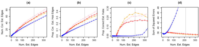
Binary network simulation with n = 100 and p = 50. Details of the axis labels are as in Figure 3. The colored lines correspond to the ℓ₁-penalized pseudo-likelihood proposal of Höfling and Tibshirani (2009) ( ); and HBN with λ₃ = 15 ( ), λ₃ = 25 ( ), and λ₃ = 30 ( ).

6. Real Data Application

We now apply HGL to a university webpage data set, and a brain cancer data set.

6.1 Application to University Webpage Data

We applied HGL to the university webpage data set from the “World Wide Knowledge Base” project at Carnegie Mellon University. This data set was pre-processed by Cardoso-Cachopo (2009). The data set consists of the occurrences of various terms (words) on webpages from four computer science departments at Cornell, Texas, Washington and Wisconsin. We consider only the 544 student webpages, and select 100 terms with the largest entropy for our analysis. In what follows, we model these 100 terms as the nodes in a Gaussian graphical model.

The goal of the analysis is to understand the relationships among the terms that appear on the student webpages. In particular, we wish to identify terms that are hubs. We are not interested in identifying edges between non-hub nodes. For this reason, we fix the tuning parameter that controls the sparsity of Z at λ₁ = 0.45 such that the matrix Z is sparse. In the interest of a graph that is interpretable, we fix λ₃ = 1.5 to obtain only a few hub nodes, and then select a value of λ₂ ranging from 0.1 to 0.5 using the BIC-type criterion presented in Section 3.4. We performed HGL with the selected tuning parameters λ₁ = 0.45, λ₂ = 0.25, and λ₃ = 1.5.⁶ The estimated matrices are shown in Figure 8.

Figure 8.

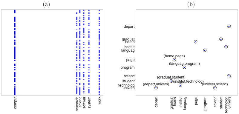
Results for HGL on the webpage data with tuning parameters selected using BIC: λ₁ = 0.45, λ₂ = 0.25, λ₃ = 1.5. Non-zero estimated values are shown, for (a): (V − diag(V)), and (b): (Z − diag(Z)).

Figure 8(a) indicates that six hub nodes are detected: comput, research, scienc, software, system, and work. For instance, the fact that comput is a hub indicates that many terms’ occurrences are explained by the occurrence of the word comput. From Figure 8(b), we see that several pairs of terms take on non-zero values in the matrix (Z−diag(Z)). These include (depart, univers); (home, page); (institut, technolog); (graduat, student); (univers, scienc), and (languag, program). These results provide an intuitive explanation of the relationships among the terms in the webpages.

6.2 Application to Gene Expression Data

We applied HGL to a publicly available cancer gene expression data set (Verhaak et al., 2010). The data set consists of mRNA expression levels for 17,814 genes in 401 patients with glioblastoma multiforme (GBM), an extremely aggressive cancer with very poor patient prognosis. Among 7,462 genes known to be associated with cancer (Rappaport et al., 2013), we selected 500 genes with the highest variance.

We aim to reconstruct the gene regulatory network that represents the interactions among the genes, as well as to identify hub genes that tend to have many interactions with other genes. Such genes likely play an important role in regulating many other genes in the network. Identifying such regulatory genes will lead to a better understanding of brain cancer, and eventually may lead to new therapeutic targets. Since we are interested in identifying hub genes, and not as interested in identifying edges between non-hub nodes, we fix λ₁ = 0.6 such that the matrix Z is sparse. We fix λ₃ = 6.5 to obtain a few hub nodes, and we select λ₂ ranging from 0.1 to 0.7 using the BIC-type criterion presented in Section 3.4.

We applied HGL with this set of tuning parameters to the empirical covariance matrix corresponding to the 401 × 500 data matrix, after standardizing each gene to have variance one. In Figure 9, we plotted the resulting network (for simplicity, only the 438 genes with at least two neighbors are displayed). We found that five genes are identified as hubs. These genes are TRIM48, TBC1D2B, PTPN2, ACRC, and ZNF763, in decreasing order of estimated edges.

Figure 9.

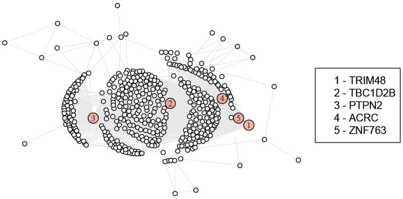
Results for HGL on the GBM data with tuning parameters selected using BIC: λ₁ = 0.6, λ₂ = 0.4, λ₃ = 6.5. Only nodes with at least two edges in the estimated network are displayed. Nodes displayed in pink were found to be hubs by the HGL algorithm.

Interestingly, some of these genes have known regulatory roles. PTPN2 is known to be a signaling molecule that regulates a variety of cellular processes including cell growth, differentiation, mitotic cycle, and oncogenic transformation (Maglott et al., 2004). ZNF763 is a DNA-binding protein that regulates the transcription of other genes (Maglott et al., 2004). These genes do not appear to be highly-connected to many other genes in the estimate that results from applying the graphical lasso (5) to this same data set (results not shown). These results indicate that HGL can be used to recover known regulators, as well as to suggest other potential regulators that may be targets for follow-up analysis.

7. Discussion

We have proposed a general framework for estimating a network with hubs by way of a convex penalty function. The proposed framework has three tuning parameters, so that it can flexibly accommodate different numbers of hubs, sparsity levels within a hub, and connectivity levels among non-hubs. We have proposed a BIC-type quantity to select tuning parameters for our proposal. We note that tuning parameter selection in unsupervised settings remains a challenging open problem (see, e.g., Foygel and Drton, 2010; Meinshausen and Bühlmann, 2010). In practice, tuning parameters could also be set based on domain knowledge or a desire for interpretability of the resulting estimates.

The framework proposed in this paper assumes an underlying model involving a set of edges between non-hub nodes, as well as a set of hub nodes. For instance, it is believed that such hub nodes arise in biology, in which “super hubs” in transcriptional regulatory networks may play important roles (Hao et al., 2012). We note here that the underlying model of hub nodes assumed in this paper differs fundamentally from a scale-free network in which the degree of connectivity of the nodes follows a power law distribution—scale-free networks simply do not have such very highly-connected hub nodes. In fact, we have shown that existing techniques for estimating a scale-free network, such as Liu and Ihler (2011) and Defazio and Caetano (2012), cannot accommodate the very dense hubs for which our proposal is intended.

As discussed in Section 2, the hub penalty function involves decomposing a parameter matrix Θ into Z + V + V^T, where Z is a sparse matrix, and V is a matrix whose columns are entirely zero or (almost) entirely non-zero. In this paper, we used an ℓ₁ penalty on Z in order to encourage it to be sparse. In effect, this amounts to assuming that the nonhub nodes obey an Erdős-Rényi network. But our formulation could be easily modified to accommodate a different network prior for the non-hub nodes. For instance, we could assume that the non-hub nodes obey a scale-free network, using the ideas developed in Liu and Ihler (2011) and Defazio and Caetano (2012). This would amount to modeling a scale-free network with hub nodes.

In this paper, we applied the proposed framework to the tasks of estimating a Gaussian graphical model, a covariance graph model, and a binary network. The proposed framework can also be applied to other types of graphical models, such as the Poisson graphical model (Allen and Liu, 2012) or the exponential family graphical model (Yang et al., 2012a).

In future work, we will study the theoretical statistical properties of the HGL formulation. For instance, in the context of the graphical lasso, it is known that the rate of statistical convergence depends upon the maximal degree of any node in the network (Ravikumar et al., 2011). It would be interesting to see whether HGL theoretically outperforms the graphical lasso in the setting in which the true underlying network contains hubs. Furthermore, it will be of interest to study HGL’s hub recovery properties from a theoretical perspective.

An R package hglasso is publicly available on the authors’ websites and on CRAN.

Appendix A. Derivation of Algorithm 1

Recall that the scaled augmented Lagrangian for (4) takes the form

$$\begin{array}{lll}L(\mathbf{B},\stackrel{\sim }{\mathbf{B}},\mathbf{W})& =& \ell (\mathbf{X},\mathbf{\Theta })+{\lambda }_1{\Vert \mathbf{Z}-\mathrm{diag}(\mathbf{Z})\Vert }_1+{\lambda }_2{\Vert \mathbf{V}-\mathrm{diag}(\mathbf{V})\Vert }_1\\ & +& {\lambda }_3\sum _{j=1}^p{\Vert {(\mathbf{V}-\mathrm{diag}(\mathbf{V}))}_j\Vert }_2+g(\stackrel{\sim }{\mathbf{B}})+\frac{\rho }{2}{\Vert \mathbf{B}-\stackrel{\sim }{\mathbf{B}}+\mathbf{W}\Vert }_F^2.\end{array}$$ (13)

The proposed ADMM algorithm requires the following updates:

1. $${\mathbf{B}}^{(t+1)}\leftarrow \underset{\mathbf{B}}{\mathrm{argmin}}L(\mathbf{B},{\stackrel{\sim }{\mathbf{B}}}^t,{\mathbf{W}}^t),$$
2. $${\stackrel{\sim }{\mathbf{B}}}^{(t+1)}\leftarrow \underset{\stackrel{\sim }{\mathbf{B}}}{\mathrm{argmin}}L({\mathbf{B}}^{(t+1)},\stackrel{\sim }{\mathbf{B}},{\mathbf{W}}^t),$$

3. W^(t+1) ← W^t + B^(t+1) − B̃^(t+1).

We now proceed to derive the updates for B and B̃.

Updates for B

To obtain updates for B = (Θ, V, Z), we exploit the fact that (13) is separable in Θ, V, and Z. Therefore, we can simply update with respect to Θ, V, and Z one-at-a-time. Update for Θ depends on the form of the convex loss function, and is addressed in the main text. Updates for V and Z can be easily seen to take the form given in Algorithm 1.

Updates for B̃

Minimizing the function in (13) with respect to B̃ is equivalent to

$$\begin{array}{ll}\underset{\stackrel{\sim }{\mathbf{\Theta }},\stackrel{\sim }{\mathbf{V}},\stackrel{\sim }{\mathbf{Z}}}{\mathrm{minimize}}& \left\{\frac{\rho }{2}{\Vert \mathbf{\Theta }-\stackrel{\sim }{\mathbf{\Theta }}+{\mathbf{W}}_1\Vert }_F^2+\frac{\rho }{2}{\Vert \mathbf{V}-\stackrel{\sim }{\mathbf{V}}+{\mathbf{W}}_2\Vert }_F^2+\frac{\rho }{2}{\Vert \mathbf{Z}-\stackrel{\sim }{\mathbf{Z}}+{\mathbf{W}}_3\Vert }_F^2\right\}\\ \mathrm{subject\; to}& \stackrel{\sim }{\mathbf{\Theta }}=\stackrel{\sim }{\mathbf{Z}}+\stackrel{\sim }{\mathbf{V}}+{\stackrel{\sim }{\mathbf{V}}}^T.\end{array}$$ (14)

Let Γ be the p × p Lagrange multiplier matrix for the equality constraint. Then, the Lagrangian for (14) is

$$\frac{\rho }{2}{\Vert \mathbf{\Theta }-\stackrel{\sim }{\mathbf{\Theta }}+{\mathbf{W}}_1\Vert }_F^2+\frac{\rho }{2}{\Vert \mathbf{V}-\stackrel{\sim }{\mathbf{V}}+{\mathbf{W}}_2\Vert }_F^2+\frac{\rho }{2}{\Vert \mathbf{Z}-\stackrel{\sim }{\mathbf{Z}}+{\mathbf{W}}_3\Vert }_F^2+\langle \mathbf{\Gamma },\stackrel{\sim }{\mathbf{\Theta }}-\stackrel{\sim }{\mathbf{Z}}-\stackrel{\sim }{\mathbf{V}}-{\stackrel{\sim }{\mathbf{V}}}^T\rangle .$$

A little bit of algebra yields

$$\begin{array}{c}\stackrel{\sim }{\mathbf{\Theta }}=\mathbf{\Theta }+{\mathbf{W}}_1-\frac{1}{\rho }\mathbf{\Gamma }\mathbf{,}\\ \stackrel{\sim }{\mathbf{V}}=\frac{1}{\rho }(\mathbf{\Gamma }+{\mathbf{\Gamma }}^T)+\mathbf{V}+{\mathbf{W}}_2,\\ \stackrel{\sim }{\mathbf{Z}}=\frac{1}{\rho }\mathbf{\Gamma }+\mathbf{Z}+{\mathbf{W}}_3,\end{array}$$

where $\mathbf{\Gamma }=\frac{\rho }{6}[(\mathbf{\Theta }+{\mathbf{W}}_1)-(\mathbf{V}+{\mathbf{W}}_2)-{(\mathbf{V}+{\mathbf{W}}_2)}^T-(\mathbf{Z}+{\mathbf{W}}_3)]$.

Appendix B. Conditions for HGL Solution to be Block-Diagonal

We begin by introducing some notation. Let ∥V∥_u,υ be the ℓ_u/ℓ_υ norm of a matrix V. For instance, ${\Vert \mathbf{V}\Vert }_{1,q}={\sum }_{j=1}^p{\Vert {\mathbf{V}}_j\Vert }_q$. We define the support of a matrix Θ as follows: supp(Θ) = {(i, j) : Θ_ij ≠ 0}. We say that Θ is supported on a set G if supp(Θ) ⊆ G. Let {C₁, …, C_K} be a partition of the index set {1, …, p}, and let $T={\cup }_{k=1}^K\{C_k\times C_k\}$. We let A_T denote the restriction of the matrix A to the set T : that is, (A_T)_ij = 0 if (i, j) ∉ T and (A_T)_ij = A_ij if (i, j) ∈ T. Note that any matrix supported on T is block-diagonal with K blocks, subject to some permutation of its rows and columns. Also, let $S_{\max }=\underset{(i,j)\in T^c}{\max }|S_{\mathit{ij}}|$.

Define

$$\begin{array}{cccc}\stackrel{\sim }{\mathbf{P}}(\mathbf{\Theta })& =& \underset{\mathbf{V},\mathbf{Z}}{\min }& {\Vert \mathbf{Z}-\mathrm{diag}(\mathbf{Z})\Vert }_1+{\widehat{\lambda }}_2{\Vert \mathbf{V}-\mathrm{diag}(\mathbf{V})\Vert }_1+{\widehat{\lambda }}_3{\Vert \mathbf{V}-\mathrm{diag}(\mathbf{V})\Vert }_{1,q}\hfill \\ & & \mathrm{subject\; to}\hfill & \mathbf{\Theta }=\mathbf{Z}+\mathbf{V}+{\mathbf{V}}^T,\hfill \end{array}$$ (15)

where ${\widehat{\lambda }}_2=\frac{{\lambda }_2}{{\lambda }_1}$ and ${\widehat{\lambda }}_3=\frac{{\lambda }_3}{{\lambda }_1}$. Then, optimization problem (6) is equivalent to

$$\underset{\mathbf{\Theta }\in \mathit{S}}{\mathrm{minimize}}-\mathrm{log\; det}(\mathbf{\Theta })+\langle \mathbf{\Theta },\mathbf{S}\rangle +{\lambda }_1\stackrel{\sim }{\mathbf{P}}(\mathbf{\Theta }),$$ (16)

where S = {Θ : Θ ≻ 0, Θ = Θ^T}.

Proof of Theorem 1 (Sufficient Condition)

Proof

First, we note that if (Θ, V, Z) is a feasible solution to (6), then (Θ_T, V_T, Z_T) is also a feasible solution to (6). Assume that (Θ, V, Z) is not supported on T. We want to show that the objective value of (6) evaluated at (Θ_T, V_T, Z_T) is smaller than the objective value of (6) evaluated at (Θ, V, Z). By Fischer’s inequality (Horn and Johnson, 1985),

$$-\mathrm{log\; det}(\mathbf{\Theta })\ge -\mathrm{log\; det}({\mathbf{\Theta }}_T).$$

Therefore, it remains to show that

$$\begin{array}{rr}\langle \mathbf{\Theta },\mathbf{S}\rangle +{\lambda }_1{\Vert \mathbf{Z}-\mathrm{diag}(\mathbf{Z})\Vert }_1+{\lambda }_2{\Vert \mathbf{V}-\mathrm{diag}(\mathbf{V})\Vert }_1+{\lambda }_3{\Vert \mathbf{V}-\mathrm{diag}(\mathbf{V})\Vert }_{1,q}& >\\ \langle {\mathbf{\Theta }}_T,\mathbf{S}\rangle +{\lambda }_1{\Vert {\mathbf{Z}}_T-\mathrm{diag}({\mathbf{Z}}_T)\Vert }_1+{\lambda }_2{\Vert {\mathbf{V}}_T-\mathrm{diag}({\mathbf{V}}_T)\Vert }_1+{\lambda }_3{\Vert {\mathbf{V}}_T-\mathrm{diag}({\mathbf{V}}_T)\Vert }_{1,q},& \end{array}$$

or equivalently, that

$$\langle {\mathbf{\Theta }}_{T^c},\mathbf{S}\rangle +{\lambda }_1{\Vert {\mathbf{Z}}_{T^c}\Vert }_1+{\lambda }_2{\Vert {\mathbf{V}}_{T^c}\Vert }_1+{\lambda }_3({\Vert \mathbf{V}-\mathrm{diag}(\mathbf{V})\Vert }_{1,q}-{\Vert {\mathbf{V}}_T-\mathrm{diag}({\mathbf{V}}_T)\Vert }_{1,q})>0.$$

Since ∥V − diag(V) ∥_1,q ≥ ∥V_T − diag(V_T)∥_1,q, it suffices to show that

$$\langle {\mathbf{\Theta }}_{T^c},\mathbf{S}\rangle +{\lambda }_1{\Vert {\mathbf{Z}}_{T^c}\Vert }_1+{\lambda }_2{\Vert {\mathbf{V}}_{T^c}\Vert }_1>0.$$ (17)

Note that 〈Θ_T^c, S〉 = 〈Θ_T^c, S_T^c〉. By the sufficient condition, S_max < λ₁ and 2S_max < λ₂.

In addition, we have that

$$\begin{array}{lll}|\langle {\mathbf{\Theta }}_{T^c},\mathbf{S}\rangle |& =& |\langle {\mathbf{\Theta }}_{T^c},{\mathbf{S}}_{T^c}\rangle |\\ & =& |\langle {\mathbf{V}}_{T^c}+{\mathbf{V}}_{T^c}^T+{\mathbf{Z}}_{T^c},{\mathbf{S}}_{T^c}\rangle |\\ & =& |\langle 2{\mathbf{V}}_{T^c}+{\mathbf{Z}}_{T^c},{\mathbf{S}}_{T^c}\rangle |\\ & \le & (2{\Vert {\mathbf{V}}_{T^c}\Vert }_1+{\Vert {\mathbf{Z}}_{T^c}\Vert }_1)S_{\max }\\ & <& {\lambda }_2{\Vert {\mathbf{V}}_{T^c}\Vert }_1+{\lambda }_1{\Vert {\mathbf{Z}}_{T^c}\Vert }_1,\end{array}$$

where the last inequality follows from the sufficient condition. We have shown (17) as desired.

Proof of Theorem 2 (Necessary Condition)

We first present a simple lemma for proving Theorem 2. Throughout the proof of Theorem 2, ∥·∥_∞ indicates the maximal absolute element of a matrix and ∥·∥_∞,s indicates the dual norm of ∥·∥_1,q.

Lemma 7

The dual representation of P̃(Θ) in (15) is

$$\begin{array}{cccc}{\stackrel{\sim }{\mathbf{P}}}^{\ast }(\mathbf{\Theta })& =& \underset{\mathbf{X},\mathbf{Y},\mathbf{\Lambda }}{\max }& \langle \mathbf{\Lambda },\mathbf{\Theta }\rangle \hfill \\ & & \mathrm{subject\; to}& \mathbf{\Lambda }+{\mathbf{\Lambda }}^T={\widehat{\lambda }}_2\mathbf{X}+{\widehat{\lambda }}_3\mathbf{Y}\hfill \\ & & & {\Vert \mathbf{X}\Vert }_{\infty }\le 1,{\Vert \mathbf{\Lambda }\Vert }_{\infty }\le 1,{\Vert \mathbf{Y}\Vert }_{\infty ,s}\le 1\hfill \\ & & & X_{\mathit{ii}}=0,Y_{\mathit{ii}}=0,{\mathrm{\Lambda }}_{\mathit{ii}}=0\mathit{for}i=1,\dots ,p,\hfill \end{array}$$ (18)

where $\frac{1}{s}+\frac{1}{q}=1$.

Proof

We first state the dual representations for the norms in (15):

$$\begin{array}{cccc}{\Vert \mathbf{Z}-\mathrm{diag}(\mathbf{Z})\Vert }_1& =& \underset{\mathbf{\Lambda }}{\max }& \langle \mathbf{\Lambda },\mathbf{Z}\rangle \hfill \\ & & \mathrm{subject\; to}& {\Vert \mathbf{\Lambda }\Vert }_{\infty }\le 1,{\mathbf{\Lambda }}_{\mathit{ii}}=0\mathrm{for}i=1,\dots ,p,\hfill \end{array}$$

$$\begin{array}{cccc}{\Vert \mathbf{V}-\mathrm{diag}(\mathbf{V})\Vert }_1& =& \underset{\mathbf{X}}{\max }& \langle \mathbf{X},\mathbf{V}\rangle \hfill \\ & & \mathrm{subject\; to}& {\Vert \mathbf{X}\Vert }_{\infty }\le 1,X_{\mathit{ii}}=0\mathrm{for}i=1,\dots ,p,\hfill \end{array}$$

$$\begin{array}{cccc}{\Vert \mathbf{V}-\mathrm{diag}(\mathbf{V})\Vert }_{1,q}& =& \underset{\mathbf{Y}}{\max }& \langle \mathbf{Y},\mathbf{V}\rangle \hfill \\ & & \mathrm{subject\; to}& {\Vert \mathbf{Y}\Vert }_{\infty ,s}\le 1,Y_{\mathit{ii}}=0\mathrm{for}i=1,\dots ,p.\hfill \end{array}$$

Then,

$$\begin{array}{l}\\ \begin{array}{cccc}\stackrel{\sim }{\mathbf{P}}(\mathbf{\Theta })& =& \underset{\mathbf{V},\mathbf{Z}}{\min }& {\Vert \mathbf{Z}-\mathrm{diag}(\mathbf{Z})\Vert }_1+{\widehat{\lambda }}_2{\Vert \mathbf{V}-\mathrm{diag}(\mathbf{V})\Vert }_1+{\widehat{\lambda }}_3{\Vert \mathbf{V}-\mathrm{diag}(\mathbf{V})\Vert }_{1,q}\hfill \\ & & \mathrm{subject\; to}& \mathbf{\Theta }=\mathbf{Z}+\mathbf{V}+{\mathbf{V}}^T\hfill \\ & =& \underset{\mathbf{V},\mathbf{Z}}{\min }& \underset{\mathbf{\Lambda },\mathbf{X},\mathbf{Y}}{\max }\langle \mathbf{\Lambda },\mathbf{Z}\rangle +{\widehat{\lambda }}_2\langle \mathbf{X},\mathbf{V}\rangle +{\widehat{\lambda }}_3\langle \mathbf{Y},\mathbf{V}\rangle \hfill \\ & & \mathrm{subject\; to}& {\Vert \mathbf{\Lambda }\Vert }_{\infty }\le 1,{\Vert \mathbf{X}\Vert }_{\infty }\le 1,{\Vert \mathbf{Y}\Vert }_{\infty ,s}\le 1\hfill \\ & & & {\mathrm{\Lambda }}_{\mathit{ii}}=0,X_{\mathit{ii}}=0,Y_{\mathit{ii}}=0\mathrm{for}i=1,\dots ,p\hfill \\ & & & \mathbf{\Theta }=\mathbf{Z}+\mathbf{V}+{\mathbf{V}}^T\hfill \\ & =& \underset{\mathbf{\Lambda },\mathbf{X},\mathbf{Y}}{\max }& \underset{\mathbf{V},\mathbf{Z}}{\min }\langle \mathbf{\Lambda },\mathbf{Z}\rangle +{\widehat{\lambda }}_2\langle \mathbf{X},\mathbf{V}\rangle +{\widehat{\lambda }}_3\langle \mathbf{Y},\mathbf{V}\rangle \hfill \\ & & \mathrm{subject\; to}& {\Vert \mathbf{\Lambda }\Vert }_{\infty }\le 1,{\Vert \mathbf{X}\Vert }_{\infty }\le 1,{\Vert \mathbf{Y}\Vert }_{\infty ,s}\le 1\hfill \\ & & & {\mathrm{\Lambda }}_{\mathit{ii}}=0,X_{\mathit{ii}}=0,Y_{\mathit{ii}}=0\mathrm{for}i=1,\dots ,p\hfill \\ & & & \mathbf{\Theta }=\mathbf{Z}+\mathbf{V}+{\mathbf{V}}^T\hfill \\ & =& \underset{\mathbf{\Lambda },\mathbf{X},\mathbf{Y}}{\max }& \langle \mathbf{\Lambda },\mathbf{\Theta }\rangle \hfill \\ & & \mathrm{subject\; to}& \mathbf{\Lambda }+{\mathbf{\Lambda }}^T={\widehat{\lambda }}_2\mathbf{X}+{\widehat{\lambda }}_3\mathbf{Y}\hfill \\ & & & {\Vert \mathbf{X}\Vert }_{\infty }\le 1,{\Vert \mathbf{\Lambda }\Vert }_{\infty }\le 1,{\Vert \mathbf{Y}\Vert }_{\infty ,s}\le 1\hfill \\ & & & X_{\mathit{ii}}=0,Y_{\mathit{ii}}=0,{\mathrm{\Lambda }}_{\mathit{ii}}=0\mathrm{for}i=1,\dots ,p.\hfill \end{array}\end{array}$$

The third equality holds since the constraints on (V, Z) and on (Λ, X, Y) are both compact convex sets and so by the minimax theorem, we can swap max and min. The last equality follows from the fact that

$$\begin{array}{cc}\underset{\mathbf{V},\mathbf{Z}}{\min }& \langle \mathbf{\Lambda },\mathbf{Z}\rangle +{\widehat{\lambda }}_2\langle \mathbf{X},\mathbf{V}\rangle +{\widehat{\lambda }}_3\langle \mathbf{Y},\mathbf{V}\rangle \\ \mathrm{subject\; to}& \mathbf{\Theta }=\mathbf{Z}+\mathbf{V}+{\mathbf{V}}^T\\ =& \{\begin{array}{cc}\langle \mathbf{\Lambda },\mathbf{\Theta }\rangle & \mathrm{if}\mathbf{\Lambda }+{\mathbf{\Lambda }}^T={\widehat{\lambda }}_2\mathbf{X}+{\widehat{\lambda }}_3\mathbf{Y}\\ -\infty & \mathrm{otherwise}.\end{array}\end{array}$$

We now present the proof of Theorem 2.

Proof

The optimality condition for (16) is given by

$$\mathbf{0}=-{\mathbf{\Theta }}^{-1}+\mathbf{S}+{\lambda }_1\mathbf{\Lambda },$$ (19)

where Λ is a subgradient of P̃(Θ) in (15) and the left-hand side of the above equation is a zero matrix of size p × p.

Now suppose that Θ* that solves (19) is supported on T, i.e., ${\mathbf{\Theta }}_{T^c}^{\ast }=0$. Then for any (i, j) ∈ T^c, we have that

$$0=S_{\mathit{ij}}+{\lambda }_1{\mathrm{\Lambda }}_{\mathit{ij}}^{\ast },$$ (20)

where Λ* is a subgradient of P̃(Θ*). Note that Λ* must be an optimal solution to the optimization problem (18). Therefore, it is also a feasible solution to (18), implying that

$$\begin{array}{lll}\hfill |{\mathrm{\Lambda }}_{\mathit{ij}}^{\ast }+{\mathrm{\Lambda }}_{\mathit{ji}}^{\ast }|& \le & {\widehat{\lambda }}_2+{\widehat{\lambda }}_3,\\ \hfill |{\mathrm{\Lambda }}_{\mathit{ij}}^{\ast }|& \le & 1.\end{array}$$

From (20), we have that ${\mathrm{\Lambda }}_{\mathit{ij}}^{\ast }=-\frac{S_{\mathit{ij}}}{{\lambda }_1}$ and thus,

$$\begin{array}{lll}{\lambda }_1& \ge & {\lambda }_1\underset{(i,j)\in T^c}{\max }|{\mathrm{\Lambda }}_{\mathit{ij}}^{\ast }|\\ & =& {\lambda }_1\underset{(i,j)\in T^c}{\max }\frac{|S_{\mathit{ij}}|}{{\lambda }_1}\\ & =& S_{\max }.\end{array}$$

Also, recall that ${\widehat{\lambda }}_2=\frac{{\lambda }_2}{{\lambda }_1}$ and ${\widehat{\lambda }}_3=\frac{{\lambda }_3}{{\lambda }_1}$. We have that

$$\begin{array}{lll}{\lambda }_2+{\lambda }_3& \ge & {\lambda }_1\underset{(i,j)\in T^c}{\max }|{\mathrm{\Lambda }}_{\mathit{ij}}^{\ast }+{\mathrm{\Lambda }}_{\mathit{ji}}^{\ast }|\\ & =& {\lambda }_1\underset{(i,j)\in T^c}{\max }\frac{2|S_{\mathit{ij}}|}{{\lambda }_1}\\ & =& 2S_{\max }.\end{array}$$

Hence, we obtain the desired result.

Appendix C. Some Properties of HGL

Proof of Lemma 3

Proof

Let (Θ*, Z*, V*) be the solution to (6) and suppose that Z* is not a diagonal matrix. Note that Z* is symmetric since Θ ∈ S ≡ {Θ : Θ ≻ 0 and Θ = Θ^T}. Let Ẑ = diag(Z*), a matrix that contains the diagonal elements of the matrix Z*. Also, construct V̂ as follows,

$${\widehat{\mathbf{V}}}_{\mathit{ij}}=\{\begin{array}{cc}{\mathbf{V}}_{\mathit{ij}}^{\ast }+\frac{{\mathbf{Z}}_{\mathit{ij}}^{\ast }}{2}& \mathrm{if}i\ne j\\ {\mathbf{V}}_{\mathit{ij}}^{\ast }& \mathrm{otherwise}.\end{array}$$

Then, we have that Θ* = Ẑ + V̂ + V̂^T. Thus, (Θ*, Ẑ, V̂) is a feasible solution to (6). We now show that (Θ*, Ẑ, V̂) has a smaller objective than (Θ*, Z*, V*) in (6), giving us a contradiction. Note that

$$\begin{array}{lll}{\lambda }_1{\Vert \widehat{\mathbf{Z}}-\mathrm{diag}(\widehat{\mathbf{Z}})\Vert }_1+{\lambda }_2{\Vert \widehat{\mathbf{V}}-\mathrm{diag}(\widehat{\mathbf{V}})\Vert }_1& =& {\lambda }_2{\Vert \widehat{\mathbf{V}}-\mathrm{diag}(\widehat{\mathbf{V}})\Vert }_1\\ & =& {\lambda }_2{\sum }_{i\ne j}|{\mathbf{V}}_{\mathit{ij}}^{\ast }+\frac{{\mathbf{Z}}_{\mathit{ij}}^{\ast }}{2}|\\ & \le & {\lambda }_2{\Vert {\mathbf{V}}^{\ast }-\mathrm{diag}({\mathbf{V}}^{\ast })\Vert }_1+\frac{{\lambda }_2}{2}{\Vert {\mathbf{Z}}^{\ast }-\mathrm{diag}({\mathbf{Z}}^{\ast })\Vert }_1,\end{array}$$

and

$$\begin{array}{ll}& {\lambda }_3{\sum }_{j=1}^p{\Vert {(\widehat{\mathbf{V}}-\mathrm{diag}(\widehat{\mathbf{V}}))}_j\Vert }_q\\ \le & {\lambda }_3{\sum }_{j=1}^p{\Vert {({\mathbf{V}}^{\ast }-\mathrm{diag}({\mathbf{V}}^{\ast }))}_j\Vert }_q+\frac{{\lambda }_3}{2}{\sum }_{j=1}^p{\Vert {({\mathbf{Z}}^{\ast }-\mathrm{diag}({\mathbf{Z}}^{\ast }))}_j\Vert }_q\\ \le & {\lambda }_3{\sum }_{j=1}^p{\Vert {({\mathbf{V}}^{\ast }-\mathrm{diag}({\mathbf{V}}^{\ast }))}_j\Vert }_q+\frac{{\lambda }_3}{2}{\Vert {\mathbf{Z}}^{\ast }-\mathrm{diag}({\mathbf{Z}}^{\ast })\Vert }_1,\end{array}$$

where the last inequality follows from the fact that for any vector x ∈ ℝ^p and q ≥ 1, ∥x∥_q is a nonincreasing function of q (Gentle, 2007).

Summing up the above inequalities, we get that

$$\begin{array}{rr}{\lambda }_1{\Vert \widehat{\mathbf{Z}}-\mathrm{diag}(\widehat{\mathbf{Z}})\Vert }_1+{\lambda }_2{\Vert \widehat{\mathbf{V}}-\mathrm{diag}(\widehat{\mathbf{V}})\Vert }_1+{\lambda }_3{\sum }_{j=1}^p{\Vert {(\widehat{\mathbf{V}}-\mathrm{diag}(\widehat{\mathbf{V}}))}_j\Vert }_q& \le \\ \frac{{\lambda }_2+{\lambda }_3}{2}{\Vert {\mathbf{Z}}^{\ast }-\mathrm{diag}({\mathbf{Z}}^{\ast })\Vert }_1+{\lambda }_2{\Vert {\mathbf{V}}^{\ast }-\mathrm{diag}({\mathbf{V}}^{\ast })\Vert }_1+{\lambda }_3{\sum }_{j=1}^p{\Vert {({\mathbf{V}}^{\ast }-\mathrm{diag}({\mathbf{V}}^{\ast }))}_j\Vert }_q& <\\ {\lambda }_1{\Vert {\mathbf{Z}}^{\ast }-\mathrm{diag}({\mathbf{Z}}^{\ast })\Vert }_1+{\lambda }_2{\Vert {\mathbf{V}}^{\ast }-\mathrm{diag}({\mathbf{V}}^{\ast })\Vert }_1+{\lambda }_3{\sum }_{j=1}^p{\Vert {({\mathbf{V}}^{\ast }-\mathrm{diag}({\mathbf{V}}^{\ast }))}_j\Vert }_q,& \end{array}$$

where the last inequality uses the assumption that ${\lambda }_1>\frac{{\lambda }_2+{\lambda }_3}{2}$. We arrive at a contradiction and therefore the result holds.

Proof of Lemma 4

Proof

Let (Θ*, Z*, V*) be the solution to (6) and suppose V* is not a diagonal matrix. Let V̂ = diag(V*), a diagonal matrix that contains the diagonal elements of V*. Also construct Ẑ as follows,

$${\widehat{\mathbf{Z}}}_{\mathit{ij}}=\{\begin{array}{cc}\hfill {\mathbf{Z}}_{\mathit{ij}}^{\ast }+{\mathbf{V}}_{\mathit{ij}}^{\ast }+{\mathbf{V}}_{\mathit{ji}}^{\ast }& \mathrm{if}i\ne j\\ \hfill {\mathbf{Z}}_{\mathit{ij}}^{\ast }& \mathrm{otherwise}.\end{array}$$

Then, we have that Θ* = V̂ + V̂^T +Ẑ. We now show that (Θ*, Ẑ, V̂) has a smaller objective value than (Θ*, Z*, V*) in (6), giving us a contradiction. We start by noting that

$$\begin{array}{lll}{\lambda }_1{\Vert \widehat{\mathbf{Z}}-\mathrm{diag}(\widehat{\mathbf{Z}})\Vert }_1+{\lambda }_2{\Vert \widehat{\mathbf{V}}-\mathrm{diag}(\widehat{\mathbf{V}})\Vert }_1& =& {\lambda }_1{\Vert \widehat{\mathbf{Z}}-\mathrm{diag}(\widehat{\mathbf{Z}})\Vert }_1\\ & \le & {\lambda }_1{\Vert {\mathbf{Z}}^{\ast }-\mathrm{diag}({\mathbf{Z}}^{\ast })\Vert }_1+2{\lambda }_1{\Vert {\mathbf{V}}^{\ast }-\mathrm{diag}({\mathbf{V}}^{\ast })\Vert }_1.\end{array}$$

By Holder’s Inequality, we know that x^T y ≤ ∥x∥_q ∥y∥_s where $\frac{1}{s}+\frac{1}{q}=1$ and x, y ∈ ℝ^p−1. Setting y = sign(x), we have that ${\Vert \mathbf{x}\Vert }_1\le {(p-1)}^{\frac{1}{s}}{\Vert \mathbf{x}\Vert }_q$. Consequently,

$$\frac{{\lambda }_3}{{(p-1)}^{\frac{1}{s}}}{\Vert {\mathbf{V}}^{\ast }-\mathrm{diag}({\mathbf{V}}^{\ast })\Vert }_1\le {\lambda }_3\sum _{j=1}^p{\Vert {({\mathbf{V}}^{\ast }-\mathrm{diag}({\mathbf{V}}^{\ast }))}_j\Vert }_{q.}$$

Combining these results, we have that

$$\begin{array}{l}{\lambda }_1{\Vert \widehat{\mathbf{Z}}-\mathrm{diag}(\widehat{\mathbf{Z}})\Vert }_1+{\lambda }_2{\Vert \widehat{\mathbf{V}}-\mathrm{diag}(\widehat{\mathbf{V}})\Vert }_1+{\lambda }_3\sum _{j=1}^p{\Vert {(\widehat{\mathbf{V}}-\mathrm{diag}(\widehat{\mathbf{V}}))}_j\Vert }_q\\ \le {\lambda }_1{\Vert {\mathbf{Z}}^{\ast }-\mathrm{diag}({\mathbf{Z}}^{\ast })\Vert }_1+2{\lambda }_1{\Vert {\mathbf{V}}^{\ast }-\mathrm{diag}({\mathbf{V}}^{\ast })\Vert }_1\\ <{\lambda }_1{\Vert {\mathbf{Z}}^{\ast }-\mathrm{diag}({\mathbf{Z}}^{\ast })\Vert }_1+\left({\lambda }_2+\frac{{\lambda }_3}{{(p-1)}^{\frac{1}{s}}}\right){\Vert {\mathbf{V}}^{\ast }-\mathrm{diag}({\mathbf{V}}^{\ast })\Vert }_1\\ \le {\lambda }_1{\Vert {\mathbf{Z}}^{\ast }-\mathrm{diag}({\mathbf{Z}}^{\ast })\Vert }_1+{\lambda }_2{\Vert {\mathbf{V}}^{\ast }-\mathrm{diag}({\mathbf{V}}^{\ast })\Vert }_1+{\lambda }_3\sum _{j=1}^p{\Vert {({\mathbf{V}}^{\ast }-\mathrm{diag}({\mathbf{V}}^{\ast }))}_j\Vert }_{q,}\end{array}$$

where we use the assumption that ${\lambda }_1<\frac{{\lambda }_2}{2}+\frac{{\lambda }_3}{2{(p-1)}^{\frac{1}{s}}}$. This leads to a contradiction.

Proof of Lemma 6

In this proof, we consider the case when ${\lambda }_1>\frac{{\lambda }_2+{\lambda }_3}{2}$. A similar proof technique can be used to prove the case when ${\lambda }_1<\frac{{\lambda }_2+{\lambda }_3}{2}$.

Proof

Let f(Θ, V, Z) denote the objective of (6) with q= 1, and (Θ*, V*, Z*) the optimal solution. By Lemma 3, the assumption that ${\lambda }_1>\frac{{\lambda }_2+{\lambda }_3}{2}$ implies that Z* is a diagonal matrix. Now let $\widehat{\mathbf{V}}=\frac{1}{2}({\mathbf{V}}^{\ast }+{({\mathbf{V}}^{\ast })}^T)$. Then

$$\begin{array}{ll}& f({\mathbf{\Theta }}^{\ast },\widehat{\mathbf{V}},{\mathbf{Z}}^{\ast })\\ =& -\mathrm{log\; det}{\mathbf{\Theta }}^{\ast }+\langle {\mathbf{\Theta }}^{\ast },\mathbf{S}\rangle +{\lambda }_1{\Vert {\mathbf{Z}}^{\ast }-\mathrm{diag}({\mathbf{Z}}^{\ast })\Vert }_1+({\lambda }_2+{\lambda }_3){\Vert \widehat{\mathbf{V}}-\mathrm{diag}(\widehat{\mathbf{V}})\Vert }_1\\ =& -\mathrm{log\; det}{\mathbf{\Theta }}^{\ast }+\langle {\mathbf{\Theta }}^{\ast },\mathbf{S}\rangle +\frac{{\lambda }_2+{\lambda }_3}{2}{\Vert {\mathbf{V}}^{\ast }+{\mathbf{V}}^{\ast T}-\mathrm{diag}({\mathbf{V}}^{\ast }+{\mathbf{V}}^{\ast T})\Vert }_1\\ \le & -\mathrm{log\; det}{\mathbf{\Theta }}^{\ast }+\langle {\mathbf{\Theta }}^{\ast },\mathbf{S}\rangle +({\lambda }_2+{\lambda }_3){\Vert {\mathbf{V}}^{\ast }-\mathrm{diag}({\mathbf{V}}^{\ast })\Vert }_1\\ =& f({\mathbf{\Theta }}^{\ast },{\mathbf{V}}^{\ast },{\mathbf{Z}}^{\ast })\\ \le & f({\mathbf{\Theta }}^{\ast },\widehat{\mathbf{V}},{\mathbf{Z}}^{\ast }),\end{array}$$

where the last inequality follows from the assumption that (Θ*, V*, Z*) solves (6). By strict convexity of f, this means that V* = V̂, i.e., V* is symmetric. This implies that

$$\begin{array}{lll}f({\mathbf{\Theta }}^{\ast },{\mathbf{V}}^{\ast },{\mathbf{Z}}^{\ast })& =& -\mathrm{log\; det}{\mathbf{\Theta }}^{\ast }+\langle {\mathbf{\Theta }}^{\ast },\mathbf{S}\rangle +\frac{{\lambda }_2+{\lambda }_3}{2}{\Vert {\mathbf{V}}^{\ast }+{\mathbf{V}}^{\ast T}-\mathrm{diag}({\mathbf{V}}^{\ast }+{\mathbf{V}}^{\ast T})\Vert }_1\\ & =& -\mathrm{log\; det}{\mathbf{\Theta }}^{\ast }+\langle {\mathbf{\Theta }}^{\ast },\mathbf{S}\rangle +\frac{{\lambda }_2+{\lambda }_3}{2}{\Vert {\mathbf{\Theta }}^{\ast }-\mathrm{diag}({\mathbf{\Theta }}^{\ast })\Vert }_1\\ & =& g({\mathbf{\Theta }}^{\ast }),\end{array}$$ (21)

where g(Θ) is the objective of the graphical lasso optimization problem, evaluated at Θ, with tuning parameter $\frac{{\lambda }_2+{\lambda }_3}{2}$. Suppose that Θ̃ minimizes g(Θ), and Θ* ≠ Θ̃. Then, by (21) and strict convexity of g, g(Θ*) = f(Θ*, V*, Z*) ≤ f(Θ̃, Θ̃/2, 0) = g(Θ̃) < g(Θ*), giving us a contradiction. Thus it must be that Θ̃ = Θ*.

Appendix D. Simulation Study for Hub Covariance Graph

In this section, we present the results for the simulation study described in Section 4.2 with n = 100, p = 200, and |H| = 4. We calculate the proportion of correctly estimated hub nodes with r = 40. The results are shown in Figure 10. As we can see from Figure 10, our proposal outperforms Bien and Tibshirani (2011). In particular, we can see from Figure 10(c) that Bien and Tibshirani (2011) fails to identify hub nodes.

Appendix E. Run Time Study for the ADMM algorithm for HGL

In this section, we present a more extensive run time study for the ADMM algorithm for HGL. We ran experiments with p = 100, 200, 300 and with n = p/2 on a 2.26GHz Intel Core 2 Duo machine. Results averaged over 10 replications are displayed in Figures 11(a)-(b), where the panels depict the run time and number of iterations required for the algorithm to converge, as a function of λ₁, with λ₂ = 0.5 and λ₃ = 2 fixed. The number of iterations required for the algorithm to converge is computed as the total number of iterations in Step 2 of Algorithm 1. We see from Figure 11(a) that as p increases from 100 to 300, the run times increase substantially, but never exceed several minutes. Note that these results are without using the block diagonal condition in Theorem 1.

Figure 11.

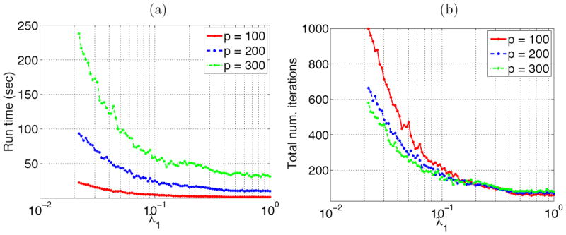
(a): Run time (in seconds) of the ADMM algorithm for HGL, as a function of λ₁, for fixed values of λ₂ and λ₃. (b): The total number of iterations required for the ADMM algorithm for HGL to converge, as a function of λ₁. All results are averaged over 10 simulated data sets. These results are without using the block diagonal condition in Theorem 1.

Appendix F. Update for Θ in Step 2(a)i for Binary Ising Model using Barzilai-Borwein Method

We consider updating Θ in Step 2(a)i of Algorithm 1 for binary Ising model. Let

$$\begin{array}{lll}h(\mathbf{\Theta })& =& -\sum _{j=1}^p\sum _{j^{\prime }=1}^p{\theta }_{j{j}^{\prime }}{({\mathbf{X}}^T\mathbf{X})}_{j{j}^{\prime }}+\sum _{i=1}^p\sum _{j=1}^p\log \left(1+\exp \left[{\theta }_{\mathit{jj}}+\sum _{j^{\prime }\ne j}{\theta }_{j{j}^{\prime }}{x}_{i{j}^{\prime }}\right]\right)\\ & & +\frac{\rho }{2}{\Vert \mathbf{\Theta }-\stackrel{\sim }{\mathbf{\Theta }}+{\mathbf{W}}_1\Vert }_F^2.\end{array}$$

Then, the optimization problem for Step 2(a)i of Algorithm 1 is

$$\underset{\mathbf{\Theta }\in \mathit{S}}{\mathrm{minimize}}h(\mathbf{\Theta }),$$ (22)

where S = {Θ : Θ = Θ^T}. In solving (22), we will treat Θ ∈ S as an implicit constraint.

The Barzilai-Borwein method is a gradient descent method with the step-size chosen to mimic the secant condition of the BFGS method (see, e.g., Barzilai and Borwein, 1988; Nocedal and Wright, 2006). The convergence of the Barzilai-Borwein method for unconstrained minimization using a non-monotone line search was shown in Raydan (1997). Recent convergence results for a quadratic cost function can be found in Dai (2013). To implement the Barzilai-Borwein method, we need to evaluate the gradient of h(Θ). Let ∇h(Θ) be a p × p matrix, where the (j, j′) entry is the gradient of h(Θ) with respect to θ_jj′, computed under the constraint Θ ∈ S, that is, θ_jj′ = θ_j′j. Then,

$${(\nabla h(\mathbf{\Theta }))}_{\mathit{jj}}=-{({\mathbf{X}}^T\mathbf{X})}_{\mathit{jj}}+\sum _{i=1}^n\left[\frac{\exp ({\theta }_{\mathit{jj}}+{{\sum }_{j^{\prime }\ne j}{\theta }_{j{j}^{\prime }}x}_{i{j}^{\prime }})}{1+\exp ({\theta }_{\mathit{jj}}+{\sum }_{j^{\prime }\ne j}{\theta }_{j{j}^{\prime }}{x}_{i{j}^{\prime }})}\right]+\rho ({\theta }_{\mathit{jj}}-{\stackrel{\sim }{\theta }}_{\mathit{jj}}+{({\mathbf{W}}_1)}_{\mathit{jj}}),$$

and

$$\begin{array}{lll}{(\nabla h(\mathbf{\Theta }))}_{j{j}^{\prime }}& =& -2{({\mathbf{X}}^T\mathbf{X})}_{\mathit{jj}}+2\rho ({\theta }_{j{j}^{\prime }}-{\stackrel{\sim }{\theta }}_{j{j}^{\prime }}+{({\mathbf{W}}_1)}_{j{j}^{\prime }})\\ & & +\sum _{i=1}^n\left[\frac{x_{i{j}^{\prime }}\exp ({\theta }_{\mathit{jj}}+{\sum }_{j^{\prime }\ne j}{\theta }_{j{j}^{\prime }}{x}_{i{j}^{\prime }})}{1+\exp ({\theta }_{\mathit{jj}}+{\sum }_{j^{\prime }\ne j}{\theta }_{j{j}^{\prime }}{x}_{i{j}^{\prime }})}+\frac{x_{\mathit{ij}}\exp ({\theta }_{j^{\prime }{j}^{\prime }}+{\sum }_{j\ne j^{\prime }}{\theta }_{j{j}^{\prime }}{x}_{\mathit{ij}})}{1+\exp ({\theta }_{j^{\prime }{j}^{\prime }}+{\sum }_{j\ne j^{\prime }}{\theta }_{j{j}^{\prime }}{x}_{\mathit{ij}})}\right].\end{array}$$

A simple implementation of the Barzilai-Borwein algorithm for solving (22) is detailed in Algorithm 2. We note that the Barzilai-Borwein algorithm can be improved (see, e.g., Barzilai and Borwein, 1988; Wright et al., 2009). We leave such improvement for future work.

Algorithm 2 Barzilai-Borwein Algorithm for Solving (22).

1. Initialize the parameters:

   1. Θ₁ = I and Θ₀ = 2I.

   2. constant τ > 0.

2. Iterate until the stopping criterion $\frac{{\Vert {\mathbf{\Theta }}_t-{\mathbf{\Theta }}_{t-1}\Vert }_F^2}{{\Vert {\mathbf{\Theta }}_{t-1}\Vert }_F^2}\le \tau$ is met, where Θ_t is the value of Θ obtained at the tth iteration:

   1. α_t = trace [(Θ_t − Θ_t−1)^T (Θ_t − Θ_t−1)] /trace [(Θ_t − Θ_t−1)^T (∇h(Θ_t) − ∇h(Θ_t−1))].

   2. Θ_t+1 = Θ_t − α_t ∇h(Θ_t).

References

- Allen GI, Liu Z. A log-linear graphical model for inferring genetic networks from high-throughput sequencing data. IEEE International Conference on Bioinformatics and Biomedicine; 2012. [Google Scholar]
- Barabási AL. Scale-free networks: A decade and beyond. Science. 2009;325:412–413. doi: 10.1126/science.1173299. [DOI] [PubMed] [Google Scholar]
- Barabási AL, Albert R. Emergence of scaling in random networks. Science. 1999;286:509–512. doi: 10.1126/science.286.5439.509. [DOI] [PubMed] [Google Scholar]
- Barzilai J, Borwein JM. Two-point step size gradient methods. IMA Journal of Numerical Analysis. 1988;8:141–148. [Google Scholar]
- Bickel PJ, Levina E. Regularized estimation of large covariance matrices. Annals of Statistics. 2008;36(1):199–227. [Google Scholar]
- Bien J, Tibshirani R. Sparse estimation of a covariance matrix. Biometrika. 2011;98(4):807–820. doi: 10.1093/biomet/asr054. [DOI] [PMC free article] [PubMed] [Google Scholar]
- Boyd S, Parikh N, Chu E, Peleato B, Eckstein J. Distributed optimization and statistical learning via the ADMM. Foundations and Trends in Machine Learning. 2010;3(1):1–122. [Google Scholar]
- Cai T, Liu W. Adaptive thresholding for sparse covariance matrix estimation. Journal of the American Statistical Association. 2011;106(494):672–684. [Google Scholar]
- Cardoso-Cachopo A. 2009 http://web.ist.utl.pt/acardoso/datasets/
- Chaudhuri S, Drton M, Richardson T. Estimation of a covariance matrix with zeros. Biometrika. 2007;94:199–216. [Google Scholar]
- Dai Y. A new analysis on the Barzilai-Borwein gradient method. Journal of the Operations Research Society of China. 2013;1(2):187–198. [Google Scholar]
- Danaher P, Wang P, Witten DM. The joint graphical lasso for inverse covariance estimation across multiple classes. Journal of the Royal Statistical Society: Series B. 2014;76(2):373–397. doi: 10.1111/rssb.12033. [DOI] [PMC free article] [PubMed] [Google Scholar]
- Defazio A, Caetano TS. A convex formulation for learning scale-free network via submodular relaxation. Advances in Neural Information Processing Systems. 2012 [Google Scholar]
- Drton M, Richardson TS. A new algorithm for maximum likelihood estimation in Gaussian graphical models for marginal independence. Proceedings of the 19th Conference on Uncertainty in Artificial Intelligence; 2003. pp. 184–191. [Google Scholar]
- Drton M, Richardson TS. Graphical methods for efficient likelihood inference in Gaussian covariance models. Journal of Machine Learning Research. 2008;9:893–914. [Google Scholar]
- Eckstein J. Augmented Lagrangian and alternating direction methods for convex optimization: A tutorial and some illustrative computational results. RUTCOR Research Reports. 2012;32 [Google Scholar]
- Eckstein J, Bertsekas DP. On the Douglas-Rachford splitting method and the proximal point algorithm for maximal monotone operators. Mathematical Programming. 1992;55(3, Ser. A):293–318. [Google Scholar]
- El Karoui N. Operator norm consistent estimation of large-dimensional sparse covariance matrices. The Annals of Statistics. 2008;36(6):2717–2756. [Google Scholar]
- Erdős P, Rényi A. On random graphs I. Publ Math Debrecen. 1959;6:290–297. [Google Scholar]
- Firouzi H, Hero AO. Local hub screening in sparse correlation graphs. Proceedings of SPIE. 2013;8858 Wavelets and Sparsity XV, 88581H. [Google Scholar]
- Foygel R, Drton M. Extended Bayesian information criteria for Gaussian graphical models. Advances in Neural Information Processing Systems. 2010 [Google Scholar]
- Friedman J, Hastie T, Tibshirani R. Sparse inverse covariance estimation with the graphical lasso. Biostatistics. 2007;9:432–441. doi: 10.1093/biostatistics/kxm045. [DOI] [PMC free article] [PubMed] [Google Scholar]
- Gentle JE. Matrix Algebra: Theory, Computations, and Applications in Statistics. Springer; New York: 2007. [Google Scholar]
- Guo J, Levina E, Michailidis G, Zhu J. Joint structure estimation for categorical Markov networks. 2010 Submitted, available at http://www.stat.lsa.umich.edu/~elevina.
- Guo J, Levina E, Michailidis G, Zhu J. Asymptotic properties of the joint neighborhood selection method for estimating categorical Markov networks. 2011 arXiv: math.PR/0000000. [Google Scholar]
- Hao D, Ren C, Li C. Revisiting the variation of clustering coefficient of biological networks suggests new modular structure. BMC System Biology. 2012;6(34):1–10. doi: 10.1186/1752-0509-6-34. [DOI] [PMC free article] [PubMed] [Google Scholar]
- Hero A, Rajaratnam B. Hub discovery in partial correlation graphs. IEEE Transactions on Information Theory. 2012;58:6064–6078. [Google Scholar]
- Höfling H, Tibshirani R. Estimation of sparse binary pairwise Markov networks using pseudo-likelihoods. Journal of Machine Learning Research. 2009;10:883–906. [PMC free article] [PubMed] [Google Scholar]
- Horn RA, Johnson CR. Matrix Analysis. Cambridge University Press; New York, NY: 1985. [Google Scholar]
- Jeong H, Mason SP, Barabási AL, Oltvai ZN. Lethality and centrality in protein networks. Nature. 2001;411:41–42. doi: 10.1038/35075138. [DOI] [PubMed] [Google Scholar]
- Lee S-I, Ganapathi V, Koller D. Efficient structure learning of Markov networks using ℓ1-regularization. Advances in Neural Information Processing Systems. 2007 [Google Scholar]
- Li L, Alderson D, Doyle JC, Willinger W. Towards a theory of scale-free graphs: Definition, properties, and implications. Internet Mathematics. 2005;2(4):431–523. [Google Scholar]
- Liljeros F, Edling CR, Amaral LAN, Stanley HE, Aberg Y. The web of human sexual contacts. Nature. 2001;411:907–908. doi: 10.1038/35082140. [DOI] [PubMed] [Google Scholar]
- Liu Q, Ihler AT. Learning scale free networks by reweighed ℓ1 regularization. Proceedings of the 14th International Conference on Artificial Intelligence and Statistics; 2011. pp. 40–48. [Google Scholar]
- Ma S, Xue L, Zou H. Alternating direction methods for latent variable Gaussian graphical model selection. Neural Computation. 2013 doi: 10.1162/NECO_a_00379. [DOI] [PubMed] [Google Scholar]
- Maglott, et al. Entrez Gene: gene-centered information at NCBI. Nucleic Acids Research. 2004;33(D):54–58. doi: 10.1093/nar/gki031. [DOI] [PMC free article] [PubMed] [Google Scholar]
- Mardia KV, Kent J, Bibby JM. Multivariate Analysis. Academic Press; 1979. [Google Scholar]
- Mazumder R, Hastie T. Exact covariance thresholding into connected components for large-scale graphical lasso. Journal of Machine Learning Research. 2012;13:781–794. [PMC free article] [PubMed] [Google Scholar]
- Meinshausen N, Bühlmann P. High dimensional graphs and variable selection with the lasso. Annals of Statistics. 2006;34(3):1436–1462. [Google Scholar]
- Meinshausen N, Bühlmann P. Stability selection. Journal of the Royal Statistical Society, Series B. 2010;72:417–473. with discussion. [Google Scholar]
- Mohan K, London P, Fazel M, Witten DM, Lee S-I. Node-based learning of Gaussian graphical models. Journal of Machine Learning Research. 2014;15:445–488. [PMC free article] [PubMed] [Google Scholar]
- Newman MEJ. The structure of scientific collaboration networks. Proceedings of the National Academy of the United States of America. 2000;98:404–409. doi: 10.1073/pnas.021544898. [DOI] [PMC free article] [PubMed] [Google Scholar]
- Nocedal J, Wright SJ. Numerical Optimization. Springer; 2006. [Google Scholar]
- Peng J, Wang P, Zhou N, Zhu J. Partial correlation estimation by joint sparse regression model. Journal of the American Statistical Association. 2009;104(486):735–746. doi: 10.1198/jasa.2009.0126. [DOI] [PMC free article] [PubMed] [Google Scholar]
- Rappaport, et al. MalaCards: an integrated compendium for diseases and their annotation. Database (Oxford) 2013 doi: 10.1093/database/bat018. [DOI] [PMC free article] [PubMed] [Google Scholar]
- Ravikumar P, Wainwright MJ, Lafferty JD. High-dimensional Ising model selection using ℓ1-regularized logistic regression. The Annals of Statistics. 2010;38(3):1287–1319. [Google Scholar]
- Ravikumar P, Wainwright MJ, Raskutti G, Yu B. High-dimensional covariance estimation by minimizing ℓ1-penalized log-determinant divergence. Electronic Journal of Statistics. 2011;5:935–980. [Google Scholar]
- Raydan M. The Barzilai and Borwein gradient method for the large scale unconstrained minimization problem. SIAM Journal on Optimization. 1997;7:26–33. [Google Scholar]
- Rothman A, Bickel PJ, Levina E, Zhu J. Sparse permutation invariant covariance estimation. Electronic Journal of Statistics. 2008;2:494–515. [Google Scholar]
- Rothman A, Levina E, Zhu J. Generalized thresholding of large covariance matrices. Journal of the American Statistical Association. 2009;104:177–186. [Google Scholar]
- Simon N, Friedman JH, Hastie T, Tibshirani R. A sparse-group lasso. Journal of Computational and Graphical Statistics. 2013;22(2):231–245. [Google Scholar]
- Tarjan R. Depth-first search and linear graph algorithms. SIAM Journal on Computing. 1972;1(2):146–160. [Google Scholar]
- Verhaak, et al. Integrated genomic analysis identifies clinically relevant subtypes of glioblastoma characterized by abnormalities in PDGFRA, IDH1, EGFR, and NF1. Cancer Cell. 2010;17(1):98–110. doi: 10.1016/j.ccr.2009.12.020. [DOI] [PMC free article] [PubMed] [Google Scholar]
- Witten DM, Friedman JH, Simon N. New insights and faster computations for the graphical lasso. Journal of Computational and Graphical Statistics. 2011;20(4):892–900. [Google Scholar]
- Wright SJ, Nowak RD, Figueiredo M. Sparse reconstruction by separable approximation. IEEE Transactions on Signal Processing. 2009;57(7):2479–2493. [Google Scholar]
- Xue L, Ma S, Zou H. Positive definite ℓ1 penalized estimation of large covariance matrices. Journal of the American Statistical Association. 2012;107(500):1480–1491. [Google Scholar]
- Yang E, Allen GI, Liu Z, Ravikumar PK. Graphical models via generalized linear models. Advances in Neural Information Processing Systems. 2012a [Google Scholar]
- Yang S, Pan Z, Shen X, Wonka P, Ye J. Fused multiple graphical lasso. 2012b arXiv:1209.2139 [cs.LG] [Google Scholar]
- Yuan M. Efficient computation of ℓ1 regularized estimates in Gaussian graphical models. Journal of Computational and Graphical Statistics. 2008;17(4):809–826. [Google Scholar]
- Yuan M, Lin Y. Model selection and estimation in the Gaussian graphical model. Biometrika. 2007a;94(10):19–35. [Google Scholar]
- Yuan M, Lin Y. Model selection and estimation in regression with grouped variables. Journal of the Royal Statistical Society, Series B. 2007b;68:49–67. [Google Scholar]
- Zou H, Hastie T, Tibshirani R. On the “degrees of freedom” of the lasso. The Annals of Statistics. 2007;35(5):2173–2192. [Google Scholar]