Graph Estimation From Multi-Attribute Data

Abstract

Undirected graphical models are important in a number of modern applications that involve exploring or exploiting dependency structures underlying the data. For example, they are often used to explore complex systems where connections between entities are not well understood, such as in functional brain networks or genetic networks. Existing methods for estimating structure of undirected graphical models focus on scenarios where each node represents a scalar random variable, such as a binary neural activation state or a continuous mRNA abundance measurement, even though in many real world problems, nodes can represent multivariate variables with much richer meanings, such as whole images, text documents, or multi-view feature vectors. In this paper, we propose a new principled framework for estimating the structure of undirected graphical models from such multivariate (or multi-attribute) nodal data. The structure of a graph is inferred through estimation of non-zero partial canonical correlation between nodes. Under a Gaussian model, this strategy is equivalent to estimating conditional independencies between random vectors represented by the nodes and it generalizes the classical problem of covariance selection (Dempster, 1972). We relate the problem of estimating non-zero partial canonical correlations to maximizing a penalized Gaussian likelihood objective and develop a method that efficiently maximizes this objective. Extensive simulation studies demonstrate the effectiveness of the method under various conditions. We provide illustrative applications to uncovering gene regulatory networks from gene and protein profiles, and uncovering brain connectivity graph from positron emission tomography data. Finally, we provide sufficient conditions under which the true graphical structure can be recovered correctly.

1. Introduction

Gaussian graphical models are commonly used to represent and explore conditional independencies between variables in a complex system. An edge between two nodes is present in the graph if and only if the corresponding variables are conditionally independent given all the other variables. Current approaches to estimating the Markov network structure underlying a Gaussian graphical model focus on cases where nodes in a network represent scalar variables such as the binary voting actions of actors (Banerjee et al., 2008; Kolar et al., 2010) or the continuous mRNA abundance measurements of genes (Peng et al., 2009). However, in many modern problems, we are interested in studying a network where nodes can represent more complex and informative vector-variables or multi-attribute entities. For example, due to advances of modern data acquisition technologies, researchers are able to measure the activities of a single gene in a high-dimensional space, such as an image of the spatial distribution of the gene expression, or a multi-view snapshot of the gene activity such as mRNA and protein abundances; when modeling a social network, a node may correspond to a person for which a vector of attributes is available, such as personal information, demographics, interests, and other features. Therefore, there is a need for methods that estimate the structure of an undirected graphical model from such multi-attribute data.

In this paper, we develop a new method for estimating the structure of undirected graphical models of which the nodes correspond to vectors, that is, multi-attribute entities. We consider the following setting. Let $X={(X_1^T,\dots ,X_p^T)}^T$ where X₁ ∈ ℝ^k₁, …, X_p ∈ ℝ^k_p are random vectors that jointly follow a multivariate Gaussian distribution with mean $\mu ={({\mu }_1^T,\dots ,{\mu }_p^T)}^T$ and covariance matrix Σ^*, which is partitioned as

$${\mathrm{\sum }}^{\ast }=\left(\begin{array}{ccc}{\mathrm{\sum }}_{11}^{\ast }& \cdots & {\mathrm{\sum }}_{1p}^{\ast }\\ ⋮& \ddots & ⋮\\ {\mathrm{\sum }}_{p1}^{\ast }& \cdots & {\mathrm{\sum }}_{pp}^{\ast }\end{array}\right),$$ (1)

with ${\mathrm{\sum }}_{ij}^{\ast }=\text{Cov}(X_i,X_j)$. Without loss of generality, we assume μ = 0. Let G = (V, E) be a graph with the vertex set V = {1, …, p} and the set of edges E ⊆ V × V that encodes the conditional independence relationships among (X_a)_a∈V. That is, each node a ∈ V of the graph G corresponds to the random vector X_a and there is no edge between nodes a and b in the graph if and only if X_a is conditionally independent of X_b given all the vectors corresponding to the remaining nodes, X_¬ab = {X_c : c ∈ V\{a, b}}. Such a graph is known as a Markov network (of Markov graph), which we shall emphasize in this paper to contrast an alternative graph over V known as the association network, which is based on pairwise marginal independence. Conditional independence can be read from the inverse of the covariance matrix of X, as the block corresponding to X_a and X_b will be equal to zero when they are conditionally independent, whereas marginal independencies are captured by the covariance matrix itself. It is well known that estimating an association network from data can result in a hard-to-interpret dense graph due to prevalent indirect correlations among variables (for example, multiple nodes each influenced by a common single node could result in a clique over all these nodes), which can be avoided in estimating a Markov network.

Let ${\mathcal{D}}_n={\left\{x_i\right\}}_{i=1}^n$ be a sample of n independent and identically distributed (iid) vectors drawn from N(0, Σ^*). For a vector x_i, we denote x_i,a ∈ ℝ^k_a the component corresponding to the node a ∈ V. Our goal is to estimate the structure of the graph G from the sample . Note that we allow for different nodes to have different number of attributes, which is useful in many applications, for example, when a node represents a gene pathway (of different sizes) in a regulatory network, or a brain region (of different volumes) in a neural activation network.

Learning the structure of a Gaussian graphical model, where each node represents a scalar random variable, is a classical problem, known as the covariance selection (Demp-ster, 1972). One can estimate the graph structure by estimating the sparsity pattern of the precision matrix Ω = Σ⁻¹. For high dimensional problems, Meinshausen and Bühlmann (2006) propose a parallel Lasso approach for estimating Gaussian graphical models by solving a collection of sparse regression problems. This procedure can be viewed as a pseudo-likelihood based method. In contrast, Banerjee et al. (2008), Yuan and Lin (2007), and Friedman et al. (2008) take a penalized likelihood approach to estimate the sparse precision matrix Ω. To reduce estimation bias, Lam and Fan (2009), Johnson et al. (2012), and Shen et al. (2012) developed the non-concave penalties to penalize the likelihood function. More recently, Yuan (2010) and Cai et al. (2011) proposed the graphical Dantzig selector and CLIME, which can be solved by linear programming and are more amenable to theoretical analysis than the penalized likelihood approach. Under certain regularity conditions, these methods have proven to be graph-estimation consistent (Ravikumar et al., 2011; Yuan, 2010; Cai et al., 2011) and scalable software packages, such as glasso and huge, were developed to implement these algorithms (Zhao et al., 2012). For a recent survey see Pourahmadi (2011). However, these methods cannot be extended to handle multi-attribute data we consider here in an obvious way. For example, if the number of attributes is the same for each node, one may naively estimate one graph per attribute, however, it is not clear how to combine such graphs into a summary graph with a clear statistical interpretation. The situation becomes even more difficult when nodes correspond to objects that have different number of attributes.

In a related work, Katenka and Kolaczyk (2011) use canonical correlation to estimate association networks from multi-attribute data, however, such networks have different interpretation to undirected graphical models. In particular, as mentioned above, association networks are known to confound the direct interactions with indirect ones as they only represent marginal associations, whereas Markov networks represent conditional independence assumptions that are better suited for separating direct interactions from indirect confounders. Our work is related to the literature on simultaneous estimation of multiple Gaussian graphical models under a multi-task setting (Guo et al., 2011; Varoquaux et al., 2010; Honorio and Samaras, 2010; Chiquet et al., 2011; Danaher et al., 2014). However, the model given in (1) is different from models considered in various multi-task settings and the optimization algorithms developed in the multi-task literature do not extend to handle the optimization problem given in our setting.

Unlike the standard procedures for estimating the structure of Gaussian graphical models, for example, neighborhood selection (Meinshausen and Bühlmann, 2006) or glasso (Friedman et al., 2008), which infer the partial correlations between pairs of nodes, our proposed method estimates the graph structure based on the partial canonical correlation, which can naturally incorporate complex nodal observations. Under that the Gaussian model in (1), the estimated graph structure has the same probabilistic independence interpretations as the Gaussian graphical model over univariate nodes. The main contributions of the paper are the following. First, we introduce a new framework for learning structure of undirected graphical models from multi-attribute data. Second, we develop an efficient algorithm that estimates the structure of a graph from the observed data. Third, we provide extensive simulation studies that demonstrate the effectiveness of our method and illustrate how the framework can be used to uncover gene regulatory networks from gene and protein profiles, and to uncover brain connectivity graph from functional magnetic resonance imaging data. Finally, we provide theoretical results, which give sufficient conditions for consistent structure recovery.

2. Methodology

In this section, we propose to estimate the graph by estimating non-zero partial canonical correlation between the nodes. This leads to a penalized maximum likelihood objective, for which we develop an efficient optimization procedure.

2.1 Preliminaries

Let X_a and X_b be two multivariate random vectors. Canonical correlation is defined between X_a and X_b as

$${\rho }_c(X_a,X_b)=\underset{u\in {ℝ}^{k_a},v\in {ℝ}^{k_b}}{max}\text{corr}(u^T{X}_a,v^T{X}_b).$$

That is, computing canonical correlation between X_a and X_b is equivalent to maximizing the correlation between two linear combinations u^TX_a and v^TX_b with respect to vectors u and v. Canonical correlation can be used to measure association strength between two nodes with multi-attribute observations. For example, in Katenka and Kolaczyk (2011), a graph is estimated from multi-attribute nodal observations by elementwise thresholding the canonical correlation matrix between nodes, but such a graph estimator may confound the direct interactions with indirect ones.

In this paper, we exploit the partial canonical correlation to estimate a graph from multi-attribute nodal observations. A graph is going to be formed by connecting nodes with non-zero partial canonical correlation. Let $\widehat{A}=\text{argmin}E({\Vert X_a-A{X}_{\neg ab}\Vert }_2^2)$ and $\widehat{B}=\text{argmin}E({\Vert X_b-B{X}_{\neg ab}\Vert }_2^2)$, then the partial canonical correlation between X_a and X_b is defined as

$${\rho }_c(X_a,X_b;X_{\neg ab})=\underset{u\in {ℝ}^{k_a},v\in {ℝ}^{k_b}}{max}\text{corr}\{u^T(X_a-\widehat{A}{X}_{\neg ab}),v^T(X_b-\widehat{B}{X}_{\neg ab})\},$$ (2)

that is, the partial canonical correlation between X_a and X_b is equal to the canonical correlation between the residual vectors of X_a and X_b after the effect of X_¬ab is removed (Rao, 1969).¹

Let Ω^* = (Σ^*)⁻¹ denote the precision matrix. A simple calculation, given in Appendix B.3, shows that

$${\rho }_c(X_a,X_b;X_{\neg ab})\ne 0\text{if}\text{and}\text{only}\text{if}\underset{u\in {ℝ}^{k_a},v\in {ℝ}^{k_b}}{max}{u}^T{\mathrm{\Omega }}_{ab}^{\ast }v\ne 0$$ (3)

This implies that estimating whether the partial canonical correlation is zero or not can be done by estimating whether a block of the precision matrix is zero or not. Furthermore, under the Gaussian model in (1), vectors X_a and X_b are conditionally independent given X_¬ab if and only if partial canonical correlation is zero. A graph built on this type of inter-nodal relationship is known as a Markov network, as it captures both local and global Markov properties over all arbitrary subsets of nodes in the graph, even though the graph is built based on pairwise conditional independence properties. In Section 2.2, we use the above observations to design an algorithm that estimates the non-zero partial canonical correlation between nodes from data using the penalized maximum likelihood estimation of the precision matrix.

Based on the relationship given in (3), we can motivate an alternative method for estimating the non-zero partial canonical correlation. Let ā = {b : b ∈ V\{a}} denote the set of all nodes minus the node a. Then

$$E(X_a\mid X_{\overline{a}}=x_{\overline{a}})={\mathrm{\sum }}_{a,\overline{a}}^{\ast }{\mathrm{\sum }}_{\overline{a},\overline{a}}^{\ast ,-1}{x}_{\overline{a}}.$$

Since ${\mathrm{\Omega }}_{a,\overline{a}}^{\ast }=-{({\mathrm{\sum }}_{aa}^{\ast }-{\mathrm{\sum }}_{a,\overline{a}}^{\ast }{\mathrm{\sum }}_{\overline{a},\overline{a}}^{\ast ,-1}{\mathrm{\sum }}_{\overline{a},a}^{\ast })}^{-1}{\mathrm{\sum }}_{a,\overline{a}}^{\ast }{\mathrm{\sum }}_{\overline{a},\overline{a}}^{\ast ,-1}$, we observe that a zero block Ω_ab can be identified from the regression coefficients when each component of X_a is regressed on X_ā. We do not build an estimation procedure around this observation, however, we note that this relationship shows how one would develop a regression based analogue of the work presented in Katenka and Kolaczyk (2011).

2.2 Penalized Log-Likelihood Optimization

Based on the data , we propose to minimize the penalized negative Gaussian log-likelihood under the model in (1),

$$\underset{\mathrm{\Omega }\succ 0}{min}\left\{\text{tr}S\mathrm{\Omega }-log\mid \mathrm{\Omega }\mid +\lambda \sum _{a,b}{\Vert {\mathrm{\Omega }}_{ab}\Vert }_F\right\},$$ (4)

where $S=n^{-1}{\sum }_{i=1}^n{x}_i{x}_i^T$ is the sample covariance matrix, ||Ω_ab||_F denotes the Frobenius norm of Ω_ab and λ is a user defined parameter that controls the sparsity of the solution Ω̂. The first two terms in (4) correspond to the negative Gaussian log-likelihood, while the second term is the Frobenius norm penalty, which encourages blocks of the precision matrix to be equal to zero, similar to the way that the ℓ₂ penalty is used in the group Lasso (Yuan and Lin, 2006). Here we assume that the same number of samples is available per attribute. However, the same method can be used in cases when some samples are obtained on a subset of attributes. Indeed, we can simply estimate each element of the matrix S from available samples, treating non-measured attributes as missing completely at random (for more details see Kolar and Xing, 2012).

The dual problem to (4) is

$$\underset{\mathrm{\sum }}{max}\sum _{j\in V}{k}_j+log\mid \mathrm{\sum }\mid \text{subject}\text{to}\underset{a,b}{max}{\Vert S_{ab}-{\mathrm{\sum }}_{ab}\Vert }_F\le \lambda ,$$ (5)

where k_j is the number attributes of node j, Σ is the dual variable to Ω and |Σ| denotes the determinant of Σ. Note that the primal problem gives us an estimate of the precision matrix, while the dual problem estimates the covariance matrix. The proposed optimization procedure, described below, will simultaneously estimate the precision matrix and covariance matrix, without explicitly performing an expensive matrix inversion.

We propose to optimize the objective function in (4) using an inexact block coordinate descent procedure, inspired by Mazumder and Agarwal (2011). The block coordinate descent is an iterative procedure that operates on a block of rows and columns while keeping the other rows and columns fixed. We write

$$\mathrm{\Omega }=\left(\begin{array}{cc}{\mathrm{\Omega }}_{aa}& {\mathrm{\Omega }}_{a,\overline{a}}\\ {\mathrm{\Omega }}_{\overline{a},a}& {\mathrm{\Omega }}_{\overline{a},\overline{a}}\end{array}\right),\mathrm{\sum }=\left(\begin{array}{cc}{\mathrm{\sum }}_{aa}& {\mathrm{\sum }}_{a,\overline{a}}\\ {\mathrm{\sum }}_{\overline{a},a}& {\mathrm{\sum }}_{\overline{a},\overline{a}}\end{array}\right),S=\left(\begin{array}{cc}{S}_{aa}& S_{a,\overline{a}}\\ S_{\overline{a},a}& S_{\overline{a},\overline{a}}\end{array}\right),$$

and suppose that (Ω̃, Σ̃) are the current estimates of the precision matrix and covariance matrix. With the above block partition, we have log |Ω| = log(Ω_ā,ā) + log(Ω_aa − Ω_a,ā(Ω_ā,ā)⁻¹Ω_ā,a). In the next iteration, Ω̂ is of the form

$$\widehat{\mathrm{\Omega }}=\stackrel{\sim }{\mathrm{\Omega }}+\left(\begin{array}{cc}{\mathrm{\Delta }}_{aa}& {\mathrm{\Delta }}_{a,\overline{a}}\\ {\mathrm{\Delta }}_{\overline{a},a}& 0\end{array}\right)=\left(\begin{array}{cc}{\widehat{\mathrm{\Omega }}}_{aa}& {\widehat{\mathrm{\Omega }}}_{a,\overline{a}}\\ {\widehat{\mathrm{\Omega }}}_{\overline{a},a}& {\stackrel{\sim }{\mathrm{\Omega }}}_{\overline{a},\overline{a}}\end{array}\right),$$

and is obtained by minimizing

$$\text{tr}{S}_{aa}{\mathrm{\Omega }}_{aa}+2\text{tr}{S}_{a,\overline{a}}{\mathrm{\Omega }}_{\overline{a},a}-log\mid {\mathrm{\Omega }}_{aa}-{\mathrm{\Omega }}_{a,\overline{a}}{({\stackrel{\sim }{\mathrm{\Omega }}}_{\overline{a},\overline{a}})}^{-1}{\mathrm{\Omega }}_{\overline{a},a}\mid +\lambda {\Vert {\mathrm{\Omega }}_{aa}\Vert }_F+2\lambda \sum _{b\ne a}{\Vert {\mathrm{\Omega }}_{ab}\Vert }_F.$$ (6)

Exact minimization over the variables Ω_aa and Ω_a,ā at each iteration of the block coordinate descent procedure can be computationally expensive. Therefore, we propose to update Ω_aa and Ω_a,ā using one generalized gradient step update (see Beck and Teboulle, 2009) in each iteration. Note that the objective function in (6) is a sum of a smooth convex function and a non-smooth convex penalty so that the gradient descent method cannot be directly applied. Given a step size t, generalized gradient descent optimizes a quadratic approximation of the objective at the current iterate Ω̃, which results in the following two updates

$${\widehat{\mathrm{\Omega }}}_{aa}=\underset{{\mathrm{\Omega }}_{aa}}{\text{argmin}}\left\{\text{tr}(S_{aa}-{\mathrm{\sum }^{\sim }}_{aa}){\mathrm{\Omega }}_{aa}+\frac{1}{2t}{\Vert {\mathrm{\Omega }}_{aa}-{\stackrel{\sim }{\mathrm{\Omega }}}_{aa}\Vert }_F^2+\lambda {\Vert {\mathrm{\Omega }}_{aa}\Vert }_F\right\},\text{and}$$ (7)

$${\widehat{\mathrm{\Omega }}}_{ab}=\underset{{\mathrm{\Omega }}_{ab}}{\text{argmin}}\left\{\text{tr}(S_{ab}-{\mathrm{\sum }^{\sim }}_{ab}){\mathrm{\Omega }}_{ba}+\frac{1}{2t}{\Vert {\mathrm{\Omega }}_{ab}-{\stackrel{\sim }{\mathrm{\Omega }}}_{ab}\Vert }_F^2+\lambda {\Vert {\mathrm{\Omega }}_{ab}\Vert }_F\right\},\forall b\in \overline{a}.$$ (8)

If the resulting estimator Ω̂ is not positive definite or the update does not decrease the objective, we halve the step size t and find a new update. Once the update of the precision matrix Ω̂ is obtained, we update the covariance matrix Σ̂. Updates to the precision and covariance matrices can be found efficiently, without performing expensive matrix inversion. First, note that the solutions to (7) and (8) can be computed in a closed form as

$${\widehat{\mathrm{\Omega }}}_{aa}=(1-t\lambda /{\Vert {\stackrel{\sim }{\mathrm{\Omega }}}_{aa}+t({\mathrm{\sum }^{\sim }}_{aa}-S_{aa})\Vert }_F)+({\stackrel{\sim }{\mathrm{\Omega }}}_{aa}+t({\mathrm{\sum }^{\sim }}_{aa}-S_{aa})),\text{and}$$ (9)

$${\widehat{\mathrm{\Omega }}}_{ab}=(1-t\lambda /{\Vert {\stackrel{\sim }{\mathrm{\Omega }}}_{ab}+t({\mathrm{\sum }^{\sim }}_{ab}-S_{ab})\Vert }_F)+({\stackrel{\sim }{\mathrm{\Omega }}}_{ab}+t({\mathrm{\sum }^{\sim }}_{ab}-S_{ab})),\forall b\in \overline{a},$$ (10)

where (x)₊ = max(0, x). Next, the estimate of the covariance matrix can be updated efficiently, without inverting the whole Ω̂ matrix, using the matrix inversion lemma as follows

$$\begin{array}{l}{\widehat{\mathrm{\sum }}}_{\overline{a},\overline{a}}={({\stackrel{\sim }{\mathrm{\Omega }}}_{\overline{a},\overline{a}})}^{-1}+{({\stackrel{\sim }{\mathrm{\Omega }}}_{\overline{a},\overline{a}})}^{-1}{\widehat{\mathrm{\Omega }}}_{\overline{a},a}{({\widehat{\mathrm{\Omega }}}_{aa}-{\widehat{\mathrm{\Omega }}}_{a,\overline{a}}{({\stackrel{\sim }{\mathrm{\Omega }}}_{\overline{a},\overline{a}})}^{-1}{\widehat{\mathrm{\Omega }}}_{\overline{a},a})}^{-1}{\widehat{\mathrm{\Omega }}}_{a,\overline{a}}{({\stackrel{\sim }{\mathrm{\Omega }}}_{\overline{a},\overline{a}})}^{-1},\\ {\widehat{\mathrm{\sum }}}_{a,\overline{a}}=-{\widehat{\mathrm{\Omega }}}_{aa}{\widehat{\mathrm{\Omega }}}_{a,\overline{a}}{\widehat{\mathrm{\sum }}}_{\overline{a},\overline{a}},\\ {\widehat{\mathrm{\sum }}}_{aa}={({\widehat{\mathrm{\Omega }}}_{aa}-{\widehat{\mathrm{\Omega }}}_{a,\overline{a}}{({\stackrel{\sim }{\mathrm{\Omega }}}_{\overline{a},\overline{a}})}^{-1}{\widehat{\mathrm{\Omega }}}_{\overline{a},a})}^{-1},\end{array}$$ (11)

with ${({\stackrel{\sim }{\mathrm{\Omega }}}_{\overline{a},\overline{a}})}^{-1}={\mathrm{\sum }^{\sim }}_{\overline{a},\overline{a}}-{\mathrm{\sum }^{\sim }}_{\overline{a},a}{\mathrm{\sum }^{\sim }}_{aa}^{-1}{\mathrm{\sum }^{\sim }}_{a,\stackrel{\sim }{a}}$.

Combining all three steps we get the following algorithm:

1. Set the initial estimator Ω̃ = diag(S) and Σ̃ = Ω̃⁻¹. Set the step size t = 1.

2. For each a ∈ V perform the following:

   • Update Ω̂ using (9) and (10).

   • If Ω̂ is not positive definite, set t ← t/2 and repeat the update.

   • Update Σ̂ using (11).

3. Repeat Step 2 until the duality gap

   $$\left|\text{tr}(S\widehat{\mathrm{\Omega }})-log\mid \widehat{\mathrm{\Omega }}\mid +\lambda \sum _{a,b}{\Vert {\widehat{\mathrm{\Omega }}}_{ab}\Vert }_F-\sum _{j\in V}{k}_j-log\mid \mathrm{\sum }\mid \right|\le \epsilon ,$$

   where ε is a prefixed precision parameter (for example, ε = 10⁻³).

Finally, we form a graph Ĝ = (V, Ê) by connecting nodes with ||Ω̂_ab||_F ≠ 0.

Computational complexity of the procedure is given in Appendix A. Convergence of the above described procedure to the unique minimum of the objective function in (4) does not follow from the standard results on the block coordinate descent algorithm (Tseng, 2001) for two reasons. First, the minimization problem in (6) is not solved exactly at each iteration, since we only update Ω_aa and Ω_a,ā using one generalized gradient step update in each iteration. Second, the blocks of variables, over which the optimization is done at each iteration, are not completely separable between iterations due to the symmetry of the problem. The proof of the following convergence result is given in Appendix B.

Lemma 1

For every value of λ > 0, the above described algorithm produces a sequence of estimates {Ω̃^(t)}_t≥1 of the precision matrix that monotonically decrease the objective values given in (4). Every element of this sequence is positive definite and the sequence converges to the unique minimizer Ω̂ of (4).

2.3 Efficient Identification of Connected Components

When the target graph Ĝ is composed of smaller, disconnected components, the solution to the problem in (4) is block diagonal (possibly after permuting the node indices) and can be obtained by solving smaller optimization problems. That is, the minimizer Ω̂ can be obtained by solving (4) for each connected component independently, resulting in massive computational gains. We give necessary and sufficient condition for the solution Ω̂ of (4) to be block-diagonal, which can be easily checked by inspecting the empirical covariance matrix S.

Our first result follows immediately from the Karush-Kuhn-Tucker conditions for the optimization problem (4) and states that if Ω̂ is block-diagonal, then it can be obtained by solving a sequence of smaller optimization problems.

Lemma 2

If the solution to (4) takes the form Ω̂ = diag(Ω̂₁, Ω̂₂, …, Ω̂_l), that is, Ω̂ is a block diagonal matrix with the diagonal blocks Ω̂₁, …, Ω̂_l, then it can be obtained by solving

$$\underset{{\mathrm{\Omega }}_{l^{\prime }}\succ 0}{min}\left\{\text{tr}{S}_{l^{\prime }}{\mathrm{\Omega }}_{l^{\prime }}-log\mid {\mathrm{\Omega }}_{l^{\prime }}\mid +\lambda \sum _{a,b}{\Vert {\mathrm{\Omega }}_{ab}\Vert }_F\right\}$$

separately for each l′ = 1, …, l, where S_l′ are submatrices of S corresponding to Ω_l′.

Next, we describe how to identify diagonal blocks of Ω̂ Let = {P₁, P₂, …, P_l} be a partition of the set V and assume that the nodes of the graph are ordered in a way that if a ∈ P_j, b ∈ P_j′, j < j′, then a < b. The following lemma states that the blocks of Ω̂ can be obtained from the blocks of a thresholded sample covariance matrix.

Lemma 3

A necessary and sufficient condition for Ω̂ to be block diagonal with blocks P₁, P₂, …, P_l is that ||S_ab||_F ≤ λ for all a ∈ P_j, b ∈ P_j′, j ≠ j′.

Blocks P₁, P₂, …, P_l can be identified by forming a p × p matrix Q with elements q_ab = {||S_ab||_F > λ} and computing connected components of the graph with adjacency matrix Q. The lemma states also that given two penalty parameters λ₁ < λ₂, the set of un-connected nodes with penalty parameter λ₁ is a subset of unconnected nodes with penalty parameter λ₂. The simple check above allows us to estimate graphs on data sets with large number of nodes, if we are interested in graphs with small number of edges. However, this is often the case when the graphs are used for exploration and interpretation of complex systems. Lemma 3 is related to existing results established for speeding-up computation when learning single and multiple Gaussian graphical models (Witten et al., 2011; Mazumder and Hastie, 2012; Danaher et al., 2014). Each condition is different, since the methods optimize different objective functions.

3. Consistent Graph Identification

In this section, we provide theoretical analysis of the estimator described in Section 2.2. In particular, we provide sufficient conditions for consistent graph recovery. For simplicity of presentation, we assume that k_a = k, for all a ∈ V, that is, we assume that the same number of attributes is observed for each node. For each a = 1, …, kp, we assume that ${({\sigma }_{aa}^{\ast })}^{-1/2}{X}_a$ is sub-Gaussian with parameter γ, where ${\sigma }_{aa}^{\ast }$ is the ath diagonal element of Σ^*. Recall that Z is a sub-Gaussian random variable if there exists a constant σ ∈ (0, ∞) such that

$$E(exp(tZ))\le exp({\sigma }^2{t}^2),\text{for}\text{all}t\in ℝ.$$

Our assumptions involve the Hessian of the function f(A) = tr SA − log |A| evaluated at the true Ω^*, = (Ω^*) = (Ω^*)⁻¹ ⊗ (Ω^*)⁻¹ ∈ ℝ^(pk)2×(pk)2, with ⊗ denoting the Kronecker product, and the true covariance matrix Σ^*. The Hessian and the covariance matrix can be thought of as block matrices with blocks of size k² × k² and k × k, respectively. We will make use of the operator (·) that operates on these block matrices and outputs a smaller matrix with elements that equal to the Frobenius norm of the original blocks. For example, (Σ^*) ∈ ℝ^p×p with elements $\mathcal{C}{({\mathrm{\sum }}^{\ast })}_{ab}={\Vert {\mathrm{\sum }}_{ab}^{\ast }\Vert }_F$. Let = {(a, b) : ||Ω_ab||_F ≠ 0} and = {(a, b) : ||Ω_ab||_F = 0}. With this notation introduced, we assume that the following irrepresentable condition holds. There exists a constant α ∈ [0, 1) such that

$${\mid \mid \mid \mathcal{C}({\mathscr{H}}_{\mathcal{N}\mathcal{T}}{({\mathscr{H}}_{\mathcal{T}\mathcal{T}})}^{-1})\mid \mid \mid }_{\infty }\le 1-\alpha ,$$ (12)

where ⫴A⫴_∞ = max_iΣ_j |A_ij|. We will also need the following quantities to specify the results κ_Σ^* = ⫴ (Σ^*)⫴_∞ and ${\kappa }_{\mathscr{H}}={\mid \mid \mid \mathcal{C}({\mathscr{H}}_{\mathcal{T}\mathcal{T}}^{-1})\mid \mid \mid }_{\infty }$. These conditions extend the conditions specified in Ravikumar et al. (2011) needed for estimating graphs from single attribute observations.

We have the following result that provides sufficient conditions for the exact recovery of the graph.

Proposition 4

Let τ > 2. We set the penalty parameter λ in (4) as

$$\lambda =8k{\alpha }^{-1}{\left(128{(1+4{\gamma }^2)}^2(\underset{a}{max}{({\sigma }_{aa}^{\ast })}^2)n^{-1}(2log(2k)+\tau log(p))\right)}^{1/2}.$$

If n > C₁s²k²(1 + 8α⁻¹)²(τ log p + log 4 + 2 log k), where s is the maximal degree of nodes in G, $C_1={(48\sqrt{2}(1+4{\gamma }^2)({max}_a{\sigma }_{aa}^{\ast })max({\kappa }_{{\mathrm{\sum }}^{\ast }}{\kappa }_{\mathscr{H}},{\kappa }_{{\mathrm{\sum }}^{\ast }}^3{\kappa }_{\mathscr{H}}^2))}^2$ and

$$\underset{(a,b)\in \mathcal{T},a\ne b}{min}{\Vert {\mathrm{\Omega }}_{ab}\Vert }_F>16\sqrt{2}(1+4{\gamma }^2)(\underset{a}{max}{\sigma }_{aa}^{\ast })(1+8{\alpha }^{-1}){\kappa }_{\mathscr{H}}k{\left(\frac{\tau logp+log4+2logk}{n}\right)}^{1/2},$$

then pr(Ĝ = G) ≥ 1 − p^2−τ.

The proof of Proposition 4 is given in Appendix B. We extend the proof of Ravikumar et al. (2011) to accommodate the Frobenius norm penalty on blocks of the precision matrix. This proposition specifies the sufficient sample size and a lower bound on the Frobenius norm of the off-diagonal blocks needed for recovery of the unknown graph. Under these conditions and correctly specified tuning parameter λ, the solution to the optimization problem in (4) correctly recovers the graph with high probability. In practice, one needs to choose the tuning parameter in a data dependent way. For example, using the Bayesian information criterion. Even though our theoretical analysis obtains the same rate of convergence as that of Ravikumar et al. (2011), our method has a significantly improved finite-sample performance, as will be shown in Section 5. It remains an open question whether the sample size requirement can be improved as in the case of group Lasso (see, for example, Lounici et al., 2011). The analysis of Lounici et al. (2011) relies heavily on the special structure of the least squares regression. Hence, their method does not carry over to the more complicated objective function as in (4).

4. Interpreting Edges

We propose a post-processing step that will allow us to quantify the strength of links identified by the method proposed in Section 2.2, as well as identify important attributes that contribute to the existence of links.

For any two nodes a and b for which Ω_ab ≠ 0, we define (a, b) = {c ∈ V\{a, b} : Ω_ac ≠ 0 or Ω_bc ≠ 0}, which is the Markov blanket for the set of nodes {X_a, X_b}. Note that the conditional distribution of ${(X_a^T,X_b^T)}^T$ given X_¬ab is equal to the conditional distribution of ${(X_a^T,X_b^T)}^T$ given . Now,

$$\begin{array}{l}{\rho }_c(X_a,X_b;X_{\neg ab})={\rho }_c(X_a,X_b;X_{\mathcal{N}(a,b)})\\ =\underset{w_a\in {ℝ}^{k_a},w_b\in {ℝ}^{k_b}}{max}\text{corr}(u^T(X_a-\stackrel{\sim }{A}{X}_{\mathcal{N}(a,b)}),v^T(X_b-\stackrel{\sim }{B}{X}_{\mathcal{N}(a,b)})),\end{array}$$

where $\stackrel{\sim }{A}=\text{argmin}E({\Vert X_a-A{X}_{\mathcal{N}(a,b)}\Vert }_2^2)$ and $\stackrel{\sim }{B}=\text{argmin}E({\Vert X_b-B{X}_{\mathcal{N}(a,b)}\Vert }_2^2)$. Let Σ̄(a, b) = var(X_a, X_b | ). Now we can express the partial canonical correlation as

$${\rho }_c(X_a,X_b;X_{\mathcal{N}(a,b)})=\underset{w_a\in {ℝ}^{k_a},w_b\in {ℝ}^{k_a}}{max}\frac{w_a^T{\overline{\mathrm{\sum }}}_{ab}{w}_b}{{(w_a^T{\overline{\mathrm{\sum }}}_{aa}{w}_a)}^{1/2}{(w_b^T{\overline{\mathrm{\sum }}}_{bb}{w}_b)}^{1/2}},$$

where

$$\overline{\mathrm{\sum }}(a,b)=\left(\begin{array}{cc}{\overline{\mathrm{\sum }}}_{aa}& {\overline{\mathrm{\sum }}}_{ab}\\ {\overline{\mathrm{\sum }}}_{ba}& {\overline{\mathrm{\sum }}}_{bb}\end{array}\right).$$

The weight vectors w_a and w_b can be easily found by solving the system of eigenvalue equations

$$\{\begin{array}{c}{\overline{\mathrm{\sum }}}_{aa}^{-1}{\overline{\mathrm{\sum }}}_{ab}{\overline{\mathrm{\sum }}}_{bb}^{-1}{\overline{\mathrm{\sum }}}_{ba}{w}_a={\varphi }^2{w}_a\\ {\overline{\mathrm{\sum }}}_{bb}^{-1}{\overline{\mathrm{\sum }}}_{ba}{\overline{\mathrm{\sum }}}_{aa}^{-1}{\overline{\mathrm{\sum }}}_{ab}{w}_b={\varphi }^2{w}_b\end{array}$$ (13)

with w_a and w_b being the vectors that correspond to the maximum eigenvalue ϕ². Furthermore, we have ρ_c(X_a, X_b; ) = ϕ. Following Katenka and Kolaczyk (2011), the weights w_a, w_b can be used to access the relative contribution of each attribute to the edge between the nodes a and b. In particular, the weight (w_a,i)² characterizes the relative contribution of the ith attribute of node a to ρ_c(X_a, X_b; ).

Given an estimate (a, b) = {c ∈ V\{a, b} : Ω̂_ac ≠ 0 or Ω̂_bc ≠ 0} of the Markov blanket (a, b), we form the residual vectors

$$r_{i,a}=x_{i,a}=\check{A}{x}_{i,\widehat{\mathcal{N}}(a,b)},r_{i,b}=x_{i,b}-\check{B}{x}_{i,\widehat{N}(a,b)},$$

where Ǎ and B̌ are the least square estimators of à and B̃. Given the residuals, we form Σ̌(a, b), the empirical version of the matrix Σ̄ (a, b), by setting

$${\mathrm{\sum }^{ˇ}}_{aa}=\text{corr}({\{r_{i,a}\}}_{i\in [n]}),{\mathrm{\sum }^{ˇ}}_{bb}=\text{corr}({\{r_{i,b}\}}_{i\in [n]}),{\mathrm{\sum }^{ˇ}}_{ab}=\text{corr}({\{r_{i,a}\}}_{i\in [n]},{\{r_{i,a}\}}_{i\in [n]}).$$

Now, solving the eigenvalue system in (13) will give us estimates of the vectors w_a, w_b and the partial canonical correlation.

Note that we have described a way to interpret the elements of the off-diagonal blocks in the estimated precision matrix. The elements of the diagonal blocks, which correspond to coefficients between attributes of the same node, can still be interpreted by their relationship to the partial correlation coefficients.

5. Simulation Studies

In this section, we perform a set of simulation studies to illustrate finite sample performance of our method. We demonstrate that the scalings of (n, p, s) predicted by the theory are sharp. Furthermore, we compare against three other methods: 1) a method that uses the glasso first to estimate one graph over each of the k individual attributes and then creates an edge in the resulting graph if an edge appears in at least one of the single attribute graphs, 2) the method of Guo et al. (2011) and 3) the method of Danaher et al. (2014). We have also tried applying the glasso to estimate the precision matrix for the model in (1) and then post-processing it, so that an edge appears in the resulting graph if the corresponding block of the estimated precision matrix is non-zero. The result of this method is worse compared to the first baseline, so we do not report it here.

All the methods above require setting one or two tuning parameters that control the sparsity of the estimated graph. We select these tuning parameters by minimizing the Bayesian information criterion (Schwarz, 1978), which balances the goodness of fit of the model and its complexity, over a grid of parameter values. For our multi-attribute method, the Bayesian information criterion takes the following form

$$\text{BIC}(\lambda )=\text{tr}(S\widehat{\mathrm{\Omega }})-log\mid \widehat{\mathrm{\Omega }}\mid +\sum _{a<b}1\mathrm{I}\{{\widehat{\mathrm{\Omega }}}_{ab}\ne 0\}{k}_a{k}_{b}log(n).$$

Other methods for selecting tuning parameters are possible, like minimization of cross-validation or Akaike information criterion (Akaike, 1974). However, these methods tend to select models that are too dense.

Theoretical results given in Section 3 characterize the sample size needed for consistent recovery of the underlying graph. In particular, Proposition 4 suggests that we need n = θs²k² log(pk) samples to estimate the graph structure consistently, for some control parameter θ > 0. Therefore, if we plot the hamming distance between the true and recovered graph against θ, we expect the curves to reach zero distance for different problem sizes at a same point. We verify this on randomly generated chain and nearest-neighbors graphs.

Simulation 1

We generate data as follows. A random graph with p nodes is created by first partitioning nodes into p/20 connected components, each with 20 nodes, and then forming a random graph over these 20 nodes. A chain graph is formed by permuting the nodes and connecting them in succession, while a nearest-neighbor graph is constructed following the procedure outlined in Li and Gui (2006). That is, for each node, we draw a point uniformly at random on a unit square and compute the pairwise distances between nodes. Each node is then connected to s = 4 closest neighbors. Since some of nodes will have more than 4 adjacent edges, we randomly remove edges from nodes that have degree larger than 4 until the maximum degree of a node in a graph is 4. Once the graph is created, we construct a precision matrix, with non-zero blocks corresponding to edges in the graph. Elements of diagonal blocks are set as 0.5^|a−b|, 0 ≤ a, b ≤ k, while off-diagonal blocks have elements with the same value, 0.2 for chain graphs and 0.3/k for nearest-neighbor graph. Finally, we add ρI to the precision matrix, so that its minimum eigenvalue is equal to 0.5. Note that s = 2 for the chain graph and s = 4 for the nearest-neighbor graph. Simulation results are averaged over 100 replicates.

Figure 1 shows simulation results. Each row in the figure reports results for one method, while each column in the figure represents a different simulation setting. For the first two columns, we set k = 3 and vary the total number of nodes in the graph. The third simulation setting sets the total number of nodes p = 20 and changes the number of attributes k. In the case of the chain graph, we observe that for small sample sizes the method of Danaher et al. (2014) outperforms all the other methods. We note that the multi-attribute method is estimating many more parameters, which require large sample size in order to achieve high accuracy. However, as the sample size increases, we observe that multi-attribute method starts to outperform the other methods. In particular, for the sample size indexed by θ = 13 all the graph are correctly recovered, while other methods fail to recover the graph consistently at the same sample size. In the case of nearest-neighbor graph, none of the methods recover the graph well for small sample sizes. However, for moderate sample sizes, multi-attribute method outperforms the other methods. Furthermore, as the sample size increases none of the other methods recover the graph exactly. This suggests that the conditions for consistent graph recovery may be weaker in the multi-attribute setting.

Figure 1.

Results of Simulation 1. Average hamming distance plotted against the rescaled sample size. Off-diagonal blocks are full matrices.

From Figure 1 we can observe that for sufficiently large sample size n, multi-attribute method recovers the graph structure exactly. Next, we evaluate performance of the methods for smaller sample sizes, with the number of attributes k = 2. Figure 2 shows average F₁ score plotted against the sample size.² This figure shows more precisely performance of the methods for smaller sample sizes that are not sufficient for perfect graph recovery. Again, even though none of the methods perform well, we can observe somewhat better performance of the multi-attribute procedure.

Figure 2.

Results of Simulation 1 for smaller sample size. The number of attributes is k = 2. Average F₁ score plotted against the sample size.

5.1 Alternative Structure of Off-diagonal Blocks

In this section, we investigate performance of different estimation procedures under different assumptions on the elements of the off-diagonal blocks of the precision matrix.

Simulation 2

First, we investigate a situation where the multi-attribute method does not perform as well as the methods that estimate multiple graphical models. One such situation arises when different attributes are conditionally independent. To simulate this situation, we use the data generating approach as before, however, we make each block Ω_ab of the precision matrix Ω a diagonal matrix. Figure 3 summarizes results of the simulation. We see that the methods of Danaher et al. (2014) and Guo et al. (2011) perform better, since they are estimating much fewer parameters than the multi-attribute method. glasso does not exploit any structural information underlying the estimation problem and requires larger sample size to correctly estimate the graph than other methods.

Figure 3.

Results of Simulation 2 described in Section 5.1. Average hamming distance plotted against the rescaled sample size. Blocks Ω_ab of the precision matrix Ω are diagonal matrices.

Simulation 3

A completely different situation arises when the edges between nodes can be inferred only based on inter-attribute data, that is, when a graph based on any individual attribute is empty. To generate data under this situation, we follow the procedure as before, but with the diagonal elements of the off-diagonal blocks Ω_ab set to zero. Figure 4 summarizes results of the simulation. In this setting, we clearly see the advantage of the multi-attribute method, compared to other three methods. Furthermore, we can see that glasso does better than multi-graph methods of Danaher et al. (2014) and Guo et al. (2011). The reason is that glasso can identify edges based on inter-attribute relationships among nodes, while multi-graph methods rely only on intra-attribute relationships. This simulation illustrates an extreme scenario where inter-attribute relationships are important for identifying edges.

Figure 4.

Results of Simulation 3 described in Section 5.1. Average hamming distance plotted against the rescaled sample size. Off-diagonal blocks Ω_ab of the precision matrix Ω have zeros as diagonal elements.

Simulation 4

So far, off-diagonal blocks of the precision matrix were constructed to have constant values. Now, we use the same data generating procedure, but generate off-diagonal blocks of a precision matrix in a different way. Each element of the off-diagonal block Ω_ab is generated independently and uniformly from the set [−0.3, −0.1]∪[0.1, 0.3]. The results of the simulation are given in Figure 5. Again, qualitatively, the results are similar to those given in Figure 1, except that in this setting more samples are needed to recover the graph correctly.

Figure 5.

Results of Simulation 4 described in Section 5.1. Average hamming distance plotted against the rescaled sample size. Off-diagonal blocks Ω_ab of the precision matrix Ω have elements uniformly sampled from [−0.3, −0.1]∪[0.1, 0.3].

5.2 Different Number of Samples per Attribute

In this section, we show how to deal with a case when different number of samples is available per attribute. As noted in Section 2.2, we can treat non-measured attributes as missing completely at random (see Kolar and Xing, 2012, for more details).

Let R = (r_il)_{i∈{1,…,n},l∈{1,…,pk}} ∈ ℝ^n×pk be an indicator matrix, which denotes for each sample point x_i the components that are observed. Then we can form an estimate of the sample covariance matrix S = (σ_lk) ∈ ℝ^pk×pk as

$${\sigma }_{lk}=\frac{{\sum }_{i=1}^n{r}_{i,l}{r}_{i,k}{x}_{i,l}{x}_{i,k}}{{\sum }_{i=1}^n{r}_{i,l}{r}_{i,k}}.$$

This estimate is plugged into the objective in (4).

Simulation 5

We generate a chain graph with p = 60 nodes, construct a precision matrix associated with the graph and k = 3 attributes, and generate n = θs²k² log(pk) samples, θ > 0. Next, we generate additional 10%, 30% and 50% samples from the same model, but record only the values for the first attribute. Results of the simulation are given in Figure 6. Qualitatively, the results are similar to those presented in Figure 1.

Figure 6.

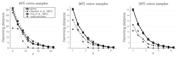
Results of Simulation 5 described in Section 5.2. Average hamming distance plotted against the rescaled sample size. Additional samples available for the first attribute.

5.3 Scale-Free Graphs

In this section, we show simulation results when the methods are applied to estimate structure of scale-free graph, that is, graph whose degree distribution follows a power low. A prominent characteristic of these graphs is presence of hub nodes.³ Such graphs commonly arise in studies of real world systems, such as gene or protein networks (Albert and Barabási, 2002).

Simulation 6

We generate a scale-free graph using the preferential attachment procedure described in Barabási and Albert (1999). The procedure starts with a 4-node cycle. New nodes are added to the graph, one at a time, and connected to nodes currently in the graph with probability proportional to their degree. Once the graph is generated, parameters in the model are set as in Simulation 1, with the number of attributes k = 2. Simulation results are summarized in Figure 7. These networks are harder to estimate using the ℓ₁-penalized procedures, due to the presence of high-degree hubs (Peng et al., 2009).

Figure 7.

Results of Simulation 6 described in Section 5.3. Average F₁ score plotted against the sample size.

6. Illustrative Applications to Real Data

In this section, we illustrate how to apply our method to data arising in studies of biological regulatory networks and Alzheimer’s disease.

6.1 Analysis of a Gene/Protein Regulatory Network

We provide illustrative, exploratory analysis of data from the well-known NCI-60 database, which contains different molecular profiles on a panel of 60 diverse human cancer cell lines. Data set consists of protein profiles (normalized reverse-phase lysate arrays for 92 antibodies) and gene profiles (normalized RNA microarray intensities from Human Genome U95 Affymetrix chip-set for 9000 genes). We focus our analysis on a subset of 91 genes/proteins for which both types of profiles are available. These profiles are available across the same set of 60 cancer cells. More detailed description of the data set can be found in Katenka and Kolaczyk (2011).

We inferred three types of networks: a network based on protein measurements alone, a network based on gene expression profiles and a single gene/protein network. For protein and gene networks we use the glasso, while for the gene/protein network, we use our procedure outlined in Section 2.2. We use the stability selection (Meinshausen and Bühlmann, 2010) procedure to estimate stable networks. In particular, we first select the penalty parameter λ using cross-validation, which over-selects the number of edges in a network. Next, we use the selected λ to estimate 100 networks based on random subsamples containing 80% of the data-points. Final network is composed of stable edges that appear in at least 95 of the estimated networks. Table 1 provides a few summary statistics for the estimated networks. Furthermore, protein and gene/protein networks share 96 edges, while gene and gene/protein networks share 104 edges. Gene and protein network share only 17 edges. Finally, 66 edges are unique to gene/protein network. Figure 8 shows node degree distributions for the three networks. We observe that the estimated networks are much sparser than the association networks in Katenka and Kolaczyk (2011), as expected due to marginal correlations between a number of nodes. The differences in networks require a closer biological inspection by a domain scientist.

Table 1.

Summary statistics for protein, gene, and gene/protein networks (p = 91).

	protein network	gene network	gene/protein network
Number of edges	122	214	249
Density	0.03	0.05	0.06
Largest connected component	62	89	82
Avg Node Degree	2.68	4.70	5.47
Avg Clustering Coefficient	0.0008	0.001	0.003

Figure 8.

Node degree distributions for protein, gene and gene/protein networks.

We proceed with a further exploratory analysis of the gene/protein network. We investigate the contribution of two nodal attributes to the existence of an edge between the nodes. Following Katenka and Kolaczyk (2011), we use a simple heuristic based on the weight vectors to classify the nodes and edges into three classes. For an edge between the nodes a and b, we take one weight vector, say w_a, and normalize it to have unit norm. Denote w_p the component corresponding to the protein attribute. Left plot in Figure 9 shows the values of $w_p^2$ over all edges. The edges can be classified into three classes based on the value of $w_p^2$. Given a threshold T, the edges for which $w_p^2\in (0,T)$ are classified as gene-influenced, the edges for which $w_p^2\in (1-T,1)$ are classified as protein influenced, while the remainder of the edges are classified as mixed type. In the left plot of Figure 9, the threshold is set as T = 0.25 following Katenka and Kolaczyk (2011). Similar classification can be performed for nodes after computing the proportion of incident edges. Let p₁, p₂ and p₃ denote proportions of gene, protein and mixed edges, respectively, incident with a node. These proportions are represented in a simplex in the right subplot of Figure 9. Nodes with mostly gene edges are located in the lower left corner, while the nodes with mostly protein edges are located in the lower right corner. Mixed nodes are located in the center and towards the top corner of the simplex. Further biological enrichment analysis is possible (see Katenka and Kolaczyk, 2011), however, we do not pursue this here.

Figure 9.

Edge and node classification based on $w_p^2$.

6.2 Uncovering Functional Brain Network

We apply our method to the Positron Emission Tomography data set, which contains 259 subjects, of whom 72 are healthy, 132 have mild cognitive Impairment and 55 are diagnosed as Alzheimer’s & Dementia. Note that mild cognitive impairment is a transition stage from normal aging to Alzheimer’s & Dementia. The data can be obtained from http://adni.loni.ucla.edu/. The preprocessing is done in the same way as in Huang et al. (2009).

Each Positron Emission Tomography image contains 91 × 109 × 91 = 902, 629 voxels. The effective brain region contains 180, 502 voxels, which are partitioned into 95 regions, ignoring the regions with fewer than 500 voxels. The largest region contains 5, 014 voxels and the smallest region contains 665 voxels. Our preprocessing stage extracts 948 representative voxels from these regions using the K-median clustering algorithm. The parameter K is chosen differently for each region, proportionally to the initial number of voxels in that region. More specifically, for each category of subjects we have an n × (d₁ + … + d₉₅) matrix, where n is the number of subjects and d₁ + … + d₉₅ = 902, 629 is the number of voxels. Next we set K_i = ⌈d_i/Σ_j dj⌉, the number of representative voxels in region i, i = 1, …, 95. The representative voxels are identified by running the K-median clustering algorithm on a sub-matrix of size n × d_i with K = K_i.

We inferred three networks, one for each subtype of subjects using the procedure outlined in Section 2.2. Note that for different nodes we have different number of attributes, which correspond to medians found by the clustering algorithm. We use the stability selection (Meinshausen and Bühlmann, 2010) approach to estimate stable networks. The stability selection procedure is combined with our estimation procedure as follows. We first select the penalty parameter λ in (4) using cross-validation, which overselects the number of edges in a network. Next, we create 100 subsampled data sets, each of which contain 80% of the data points, and estimate one network for each data set using the selected λ. The final network is composed of stable edges that appear in at least 95 of the estimated networks.

We visualize the estimated networks in Figure 10. Table 2 provides a few summary statistics for the estimated networks. Appendix C contains names of different regions, as well as the adjacency matrices for networks. From the summary statistics, we can observe that in normal subjects there are many more connections between different regions of the brain. Loss of connectivity in Alzheimer’s & Dementia has been widely reported in the literature (Greicius et al., 2004; Hedden et al., 2009; Andrews-Hanna et al., 2007; Wu et al., 2011).

Figure 10.

Brain connectivity networks

Table 2.

Summary statistics for brain connectivity networks

	Healthy subjects	Mild Cognitive Impairment	Alzheimer’s & Dementia
Number of edges	116	84	59
Density	0.030	0.020	0.014
Largest connected component	48	27	25
Avg Node Degree	2.40	1.73	1.2
Avg Clustering Coefficient	0.001	0.0023	0.0007

Learning functional brain connectivity is potentially valuable for early identification of signs of Alzheimer’s disease. Huang et al. (2009) approach this problem using exploratory data analysis. The framework of Gaussian graphical models is used to explore functional brain connectivity. Here we point out that our approach can be used for the same exploratory task, without the need to reduce the information in the whole brain to one number. For example, from our estimates, we observe the loss of connectivity in the cerebellum region of patients with Alzheimer’s disease, which has been reported previously in Sjöbeck and Englund (2001). As another example, we note increased connectivity between the frontal lobe and other regions in the patients, which was linked to compensation for the lost connections in other regions (Stern, 2006; Gould et al., 2006).

7. Conclusion and Discussion

This paper extends the classical Gaussian graphical model to handle multi-attribute data. Multi-attribute data appear naturally in social media and scientific data analysis. For example, in a study of social networks, one may use personal information, including demographics, interests, and many other features, as nodal attributes. We proposed a new family of Gaussian graphical models for modeling such multi-attribute data. The main idea is to replace the notion of partial correlation in the existing graphical model literature by partial canonical correlation. Such a modification, though simple, has profound impact to both applications and theory. Practically, many challenging data, including brain imaging and gene expression profiles, can be naturally fitted using this model, which has been illustrated in the paper. Theoretically, we proved sufficient conditions that secure the correct recovery of the unknown population network structure.

The methods and theory of this paper can be naturally extended to handle non-Gaussian data by replacing the Gaussian model with the more general nonparanormal model (Liu et al., 2009) or the transelliptical model (Liu et al., 2012). Both of them can be viewed as semiparametric extensions of the Gaussian graphical model. Instead of assuming that data follows a Gaussian distribution, one assumes that there exists a set of strictly increasing univariate functions, so that after marginal transformation the data follows a Gaussian or Elliptical distribution. More details on model interpretation can be found in Liu et al. (2009) and Liu et al. (2012). To handle multi-attribute data in this semiparametric framework, we would replace the sample covariance matrix S in Eq. (4) by a rank-based correlation matrix estimator. We leave the formal analysis of this approach for future work.

Appendix A. Complexity Analysis of Multi-attribute Estimation

Step 2 of the estimation algorithm updates portions of the precision and covariance matrices corresponding to one node at a time. We observe that the computational complexity of updating the precision matrix is (pk²). Updating the covariance matrix requires computing (Ω̃_ā,ā)⁻¹, which can be efficiently done in (p²k² + pk² + k³)= (p²k²) operations, assuming that k ≪ p. With this, the covariance matrix can be updated in (p²k²) operations. Therefore the total cost of updating the covariance and precision matrices is (p²k²) operations. Since step 2 needs to be performed for each node a ∈ V, the total complexity is (p³k²). Let T denote the total number of times step 2 is executed. This leads to the overall complexity of the algorithm as (Tp³k²). In practice, we observe that T ≈ 10 to 20 for sparse graphs. Furthermore, when the whole solution path is computed, we can use warm starts to further speed up computation, leading to T < 5 for each λ.

Appendix B. Technical Proofs

In this appendix, we collect proofs of the results presented in the main part of the paper.

B.1 Proof of Lemma 1

We start the proof by giving to technical results needed later. The following lemma states that the minimizer of (4) is unique and has bounded minimum and maximum eigenvalues, denoted Λ_min and Λ_max.

Lemma 5

For every value of λ > 0, the optimization problem in Eq. (4) has a unique minimizer Ω̂ which satisfies Λ_min(Ω̂ ≥ (Λ_max(S) + λp)⁻¹ > 0 and Λ_max(Ω̂ ≤ λ⁻¹ Σ_j∈V k_j.

Proof

The optimization objective given in (4) can be written in the equivalent constrained form as

$$\underset{\mathrm{\Omega }\succ 0}{min}\text{tr}S\mathrm{\Omega }-log\mid \mathrm{\Omega }\mid \text{subject}\text{to}\sum _{a,b}{\Vert {\mathrm{\Omega }}_{ab}\Vert }_F\le C(\lambda ).$$

The procedure involves minimizing a continuous objective over a compact set, and so by Weierstrass theorem, the minimum is always achieved. Furthermore, the objective is strongly convex and therefore the minimum is unique.

The solution Ω̂ to the optimization problem (4) satisfies

$$S-{\widehat{\mathrm{\Omega }}}^{-1}+\lambda Z=0,$$ (14)

where Z ∈ ∂ Σ_a,b ||Ω̂_ab||_F is the element of the sub-differential and satisfies ||Z_ab||_F ≤ 1 for all (a, b) ∈ V². Therefore,

$${\mathrm{\Lambda }}_{max}({\widehat{\mathrm{\Omega }}}^{-1})\le {\mathrm{\Lambda }}_{max}(S)+\lambda {\mathrm{\Lambda }}_{max}(Z)\le {\mathrm{\Lambda }}_{max}(S)+\lambda p.$$

Next, we prove an upper bound on Λ_max(Ω̂). At optimum, the primal-dual gap is zero, which gives that

$$\sum _{a,b}{\Vert {\widehat{\mathrm{\Omega }}}_{ab}\Vert }_F\le {\lambda }^{-1}(\sum _{j\in V}{k}_j-\text{tr}S\widehat{\mathrm{\Omega }})\le {\lambda }^{-1}\sum _{j\in V}{k}_j,$$

as S ⪰ 0 and Ω̂ ≻ 0. Since Λ_max(Ω̂) ≤ Σ_a,b ||Ω̂_ab||_F, the proof is done.

The next results states that the objective function has a Lipschitz continuous gradient, which will be used to show that the generalized gradient descent can be used to find Ω̂.

Lemma 6

The function f(A) = tr SA − log |A| has a Lipschitz continuous gradient on the set {A ∈ : Λ_min(A) ≥ γ}, with the Lipschitz constant L = γ⁻².

Proof

We have that ∇f(A) = S − A⁻¹. Then

$$\begin{array}{l}{\Vert \nabla f(A)-\nabla f(A^{\prime })\Vert }_F={\Vert A^{-1}-{(A^{\prime })}^{-1}\Vert }_F\\ \le {\mathrm{\Lambda }}_{max}{A}^{-1}{\Vert A-A^{\prime }\Vert }_F{\mathrm{\Lambda }}_{max}{A}^{-1}\\ \le {\gamma }^{-2}{\Vert A-A^{\prime }\Vert }_F,\end{array}$$

which completes the proof.

Now, we provide the proof of Lemma 1.

By construction, the sequence of estimates (Ω̃^(t))_t≥1 decrease the objective value and are positive definite.

To prove the convergence, we first introduce some additional notation. Let f(Ω) = tr SΩ − log |Ω| and F (Ω) = f(Ω) + Σ_ab ||Ω_ab||_F. For any L > 0, let

$$Q_L(\mathrm{\Omega };\overline{\mathrm{\Omega }}):=f(\overline{\mathrm{\Omega }})+\text{tr}[(\mathrm{\Omega }-\overline{\mathrm{\Omega }})\nabla f(\overline{\mathrm{\Omega }})]+\frac{L}{2}{\Vert \mathrm{\Omega }-\overline{\mathrm{\Omega }}\Vert }_F^2+\sum _{ab}{\Vert {\mathrm{\Omega }}_{ab}\Vert }_F$$

be a quadratic approximation of F (Ω) at a given point Ω̄, which has a unique minimizer

$$p_L(\overline{\mathrm{\Omega }}):=arg\underset{\mathrm{\Omega }}{min}{Q}_L(\mathrm{\Omega };\overline{\mathrm{\Omega }}).$$

From Lemma 2.3. in Beck and Teboulle (2009), we have that

$$F(\overline{\mathrm{\Omega }})-F(p_L(\overline{\mathrm{\Omega }}))\ge \frac{L}{2}{\Vert p_L(\overline{\mathrm{\Omega }})-\overline{\mathrm{\Omega }}\Vert }_F^2,$$ (15)

if F(p_L(Ω̄)) ≤ Q_L(p_L(Ω̄); Ω̄). Note that F(p_L(Ω̄)) ≤ Q_L(p_L(Ω̄); Ω̄) always holds if L is as large as the Lipschitz constant of ∇F.

Let Ω̃^(t−1) and Ω̃^(t) denote two successive iterates obtained by the procedure. Without loss of generality, we can assume that Ω̃^(t) is obtained by updating the rows/columns corresponding to the node a. From (15), it follows that

$$\frac{2}{L_k}(F({\stackrel{\sim }{\mathrm{\Omega }}}^{(t-1)})-F({\stackrel{\sim }{\mathrm{\Omega }}}^{(t)}))\ge {\Vert {\stackrel{\sim }{\mathrm{\Omega }}}_{aa}^{(t-1)}-{\stackrel{\sim }{\mathrm{\Omega }}}_{aa}^{(t)}\Vert }_F+2\sum _{b\ne a}{\Vert {\stackrel{\sim }{\mathrm{\Omega }}}_{ab}^{(t-1)}-{\stackrel{\sim }{\mathrm{\Omega }}}_{ab}^{(t)}\Vert }_F,$$ (16)

where L_k is a current estimate of the Lipschitz constant. Recall that in our procedure the scalar t serves as a local approximation of 1/L. Since eigenvalues of Ω̂ are bounded according to Lemma 5, we can conclude that the eigenvalues of Ω̃^(t−1) are bounded as well. Therefore the current Lipschitz constant is bounded away from zero, using Lemma 6. Combining the results, we observe that the right hand side of (16) converges to zero as t → ∞, since the optimization procedure produces iterates that decrease the objective value. This shows that ${\Vert {\stackrel{\sim }{\mathrm{\Omega }}}_{aa}^{(t-1)}-{\stackrel{\sim }{\mathrm{\Omega }}}_{aa}^{(t)}\Vert }_F+2{\sum }_{b\ne a}{\Vert {\stackrel{\sim }{\mathrm{\Omega }}}_{ab}^{(t-1)}-{\stackrel{\sim }{\mathrm{\Omega }}}_{ab}^{(t)}\Vert }_F$ converges to zero, for any a ∈ V. Since (Ω̃^(t) is a bounded sequence, it has a limit point, which we denote Ω̂. It is easy to see, from the stationary conditions for the optimization problem given in (6), that the limit point Ω̂ also satisfies the global KKT conditions to the optimization problem in (4).

B.2 Proof of Lemma 3

Suppose that the solution Ω̂ to (4) is block diagonal with blocks (P₁, P₂, … , P_l. For two nodes a, b in different blocks, we have that ${(\widehat{\mathrm{\Omega }})}_{ab}^{-1}=0$ as the inverse of the block diagonal matrix is block diagonal. From the KKT conditions, it follows that ||S_ab||_F ≤ λ.

Now suppose that ||S_ab||_F ≤ λ for all a ∈ P_j, b ∈ P_j′, j ≠ j′. For every l′ = 1, … , l construct

$${\stackrel{\sim }{\mathrm{\Omega }}}_{l^{\prime }}=arg\underset{{\mathrm{\Omega }}_{l^{\prime }}\succ 0}{min}\text{tr}{S}_{l^{\prime }}{\mathrm{\Omega }}_{l^{\prime }}-log\mid {\mathrm{\Omega }}_{l^{\prime }}\mid +\lambda \sum _{a,b}{\Vert {\mathrm{\Omega }}_{ab}\Vert }_F.$$

Then Ω̂ = diag(Ω̂₁, Ω̂₂, … , Ω̂_l) is the solution of (4) as it satisfies the KKT conditions.

B.3 Proof of Eq. (3)

First, we note that

$$var({(X_a^T,X_b^T)}^T\mid X_{\overline{ab}})={\mathrm{\sum }}_{ab,ab}-{\mathrm{\sum }}_{ab,\overline{ab}}{\mathrm{\sum }}_{\overline{ab},\overline{ab}}^{-1}{\mathrm{\sum }}_{\overline{ab},ab}$$

is the conditional covariance matrix of ${(X_a^T,X_b^T)}^T$ given the remaining nodes $X_{\overline{ab}}$ (see Proposition C.5 in Lauritzen (1996)). Define $\overline{\mathrm{\sum }}-{\mathrm{\sum }}_{ab,ab}-{\mathrm{\sum }}_{ab,\overline{ab}}{\mathrm{\sum }}_{\overline{ab},\overline{ab}}^{-1}{\mathrm{\sum }}_{\overline{ab},ab}$ . Partial canonical correlation between X_a and X_b is equal to zero if and only if Σ̄_ab = 0. On the other hand, the matrix inversion lemma gives that Ω_ab,ab = Σ̄⁻¹. Now, Ω_ab = 0 if and only if Σ̄_ab = 0. This shows the equivalence relationship in Eq. (3).

B.4 Proof of Proposition 4

We provide sufficient conditions for consistent network estimation. Proposition 4 given in Section 3 is then a simple consequence. To provide sufficient conditions, we extend the work of Ravikumar et al. (2011) to our setting, where we observe multiple attributes for each node. In particular, we extend their Theorem 1.

For simplicity of presentation, we assume that k_a = k, for all a ∈ V, that is, we assume that the same number of attributes is observed for each node. Our assumptions involve the Hessian of the function f(A) = tr SA − log |A| evaluated at the true Ω*,

$$\mathscr{H}=\mathscr{H}({\mathrm{\Omega }}^{\ast })={({\mathrm{\Omega }}^{\ast })}^{-1}\otimes {({\mathrm{\Omega }}^{\ast })}^{-1}\in {ℝ}^{{(pk)}^2\times {(pk)}^2},$$ (17)

and the true covariance matrix Σ*. The Hessian and the covariance matrix can be thought of block matrices with blocks of size k² × k² and k × k, respectively. We will make use of the operator (·) that operates on these block matrices and outputs a smaller matrix with elements that equal to the Frobenius norm of the original blocks,

$$\left(\begin{array}{cccc}{A}_{11}& A_{12}& \cdots & A_{1p}\\ A_{21}& A_{22}& \cdots & A_{2p}\\ ⋮& & \ddots & ⋮\\ A_{p1}& \cdots & & A_{pp}\end{array}\right)\stackrel{\mathcal{C}(·)}{\to }\left(\begin{array}{cccc}{\Vert A_{11}\Vert }_F& {\Vert A_{12}\Vert }_F& \cdots & {\Vert A_{1p}\Vert }_F\\ {\Vert A_{21}\Vert }_F& {\Vert A_{22}\Vert }_F& \cdots & {\Vert A_{2p}\Vert }_F\\ ⋮& & \ddots & ⋮\\ {\Vert A_{p1}\Vert }_F& \cdots & & {\Vert A_{pp}\Vert }_F\end{array}\right).$$

In particular, (Σ*) ∈ ℝ^p×p and ( ) ∈ ℝ^p2×p2.

We denote the index set of the non-zero blocks of the precision matrix as

$$\mathcal{T}:=\{(a,b)\in V\times V:{\Vert {\mathrm{\Omega }}_{ab}^{\ast }\Vert }_2\ne 0\}\cup \{(a,a):a\in V\}$$

and let denote its complement in V × V, that is,

$$\mathcal{N}=\{(a,b):{\Vert {\mathrm{\Omega }}_{ab}\Vert }_F=0\}.$$

As mentioned earlier, we need to make an assumption on the Hessian matrix, which takes the standard irrepresentable-like form. There exists a constant α ∈ [0, 1) such that

$${\mid \mid \mid \mathcal{C}({\mathscr{H}}_{\mathcal{N}\mathcal{T}}{({\mathscr{H}}_{\mathcal{T}\mathcal{T}})}^{-1})\mid \mid \mid }_{\infty }\le 1-\alpha .$$ (18)

These condition extends the irrepresentable condition given in Ravikumar et al. (2011), which was needed for estimation of networks from single attribute observations. It is worth noting, that the condition given in Eq. (18) can be much weaker than the irrepresentable condition of Ravikumar et al. (2011) applied directly to the full Hessian matrix. This can be observed in simulations done in Section 5, where a chain network is not consistently estimated even with a large number of samples.

We will also need the following two quantities to specify the results

$${\kappa }_{{\mathrm{\sum }}^{\ast }}={\mid \mid \mid \mathcal{C}({\mathrm{\sum }}^{\ast })\mid \mid \mid }_{\infty },$$ (19)

and

$${\kappa }_{\mathscr{H}}={\mid \mid \mid \mathcal{C}({\mathscr{H}}_{\mathcal{T}\mathcal{T}}^{-1})\mid \mid \mid }_{\infty }.$$ (20)

Finally, the results are going to depend on the tail bounds for the elements of the matrix (S − Σ*). We will assume that there is a constant v_* ∈ (0, ∞] and a function f: × (0, ∞) ↦ (0, ∞) such that for any (a, b) ∈ V × V

$$\text{pr}(\mathcal{C}{(S-{\mathrm{\sum }}^{\ast })}_{ab}\ge \delta )\le \frac{1}{f(n,\delta )}\delta \in (0,v_{\ast }^{-1}].$$ (21)

The function f(n, δ) will be monotonically increasing in both n and δ. Therefore, we define the following two inverse functions

$${\overline{n}}_f(\delta ;r)=\text{argmax}\{n:f(n,\delta )\le r\}$$ (22)

and

$${\overline{\delta }}_f(r;n)=argmax\{\delta :f(n,\delta )\le r\}$$ (23)

for r ∈ [1, ∞).

With the notation introduced, we have the following result.

Theorem 7

Assume that the irrepresentable condition in Eq. (18) is satisfied and that there exists a constant v_* ∈ (0, ∞] and a function f(n, δ) so that Eq. (21) is satisfied for any (a, b) ∈ V × V. Let

$$\lambda =\frac{8}{\alpha }{\overline{\delta }}_f(n,p^{\tau })$$

for some τ > 2. If

$$n>{\overline{n}}_f\left(\frac{1}{max(v_{\ast },6(1+8{\alpha }^{-1})smax({\kappa }_{{\mathrm{\sum }}^{\ast }}{\kappa }_{\mathscr{H}},{\kappa }_{{\mathrm{\sum }}^{\ast }}^3{\kappa }_{\mathscr{H}}^2))},p^{\tau }\right),$$ (24)

then

$${\Vert \mathcal{C}(\widehat{\mathrm{\Omega }}-\mathrm{\Omega })\Vert }_{\infty }\le 2(1+8{\alpha }^{-1}){\kappa }_{\mathscr{H}}{\overline{\delta }}_f(n,p^{\tau })$$ (25)

with probability at least 1 − p^2−τ.

Theorem 7 is of the same form as Theorem 1 in Ravikumar et al. (2011), but the ℓ_∞ element-wise convergence is established for (Ω̂−Ω), which will guarantee successful recovery of nonzero partial canonical correlations if the blocks of the true precision matrix are sufficiently large.

Theorem 7 is proven as Theorem 1 in Ravikumar et al. (2011). We provide technical results in Lemma 8, Lemma 9 and Lemma 10, which can be used to substitute results of Lemma 4, Lemma 5 and Lemma 6 in Ravikumar et al. (2011) under our setting. The rest of the arguments then go through. Below we provide some more details.

First, let : ℝ^pk×pk ↦ ℝ^pk×pk be the mapping defined as

$$\mathcal{Z}{(A)}_{ab}=\{\begin{array}{ll}\frac{A_{ab}}{{\Vert A_{ab}\Vert }_F}\hfill & \text{if}{\Vert A_{ab}\Vert }_F\ne 0,\hfill \\ Z\text{with}{\Vert Z\Vert }_F\le 1\hfill & \text{if}{\Vert A_{ab}\Vert }_F=0,\hfill \end{array}$$ (26)

Next, define the function

$$G(\mathrm{\Omega })=\text{tr}\mathrm{\Omega }S-log\mid \mathrm{\Omega }\mid +\lambda {\Vert \mathcal{C}(\mathrm{\Omega })\Vert }_1,\forall \mathrm{\Omega }\succ 0$$ (27)

and the following system of equations

$$\{\begin{array}{llll}{S}_{ab}-{({\mathrm{\Omega }}^{-1})}_{ab}\hfill & =\hfill & -\lambda \mathcal{Z}{(\mathrm{\Omega })}_{ab},\hfill & \text{if}{\mathrm{\Omega }}_{ab}\ne 0\hfill \\ {\Vert S_{ab}-{({\mathrm{\Omega }}^{-1})}_{ab}\Vert }_F\hfill & \le \hfill & \lambda ,\hfill & \text{if}{\mathrm{\Omega }}_{ab}=0.\hfill \end{array}$$ (28)

It is known that Ω ∈ ℝ^p̃×p̃ is the minimizer of optimization problem in Eq. (4) if and only if it satisfies the system of equations given in Eq. (28). We have already shown in Lemma 5 that the minimizer is unique.

Let Ω̃ be the solution to the following constrained optimization problem

$$\underset{\mathrm{\Omega }\succ 0}{min}\text{tr}S\mathrm{\Omega }-log\mid \mathrm{\Omega }\mid +\lambda {\Vert \mathcal{C}(\mathrm{\Omega })\Vert }_1\text{subject}\text{to}\mathcal{C}{(\mathrm{\Omega })}_{ab}=0,\forall (a,b)\in \mathcal{N}.$$ (29)

Observe that one cannot find Ω̃ in practice, as it depends on the unknown set . However, it is a useful construction in the proof. We will prove that Ω̃ is solution to the optimization problem given in Eq. (4), that is, we will show that Ω̃ satisfies the system of equations (28).

Using the first-order Taylor expansion we have that

$${\stackrel{\sim }{\mathrm{\Omega }}}^{-1}={({\mathrm{\Omega }}^{\ast })}^{-1}-{({\mathrm{\Omega }}^{\ast })}^{-1}\mathrm{\Delta }{({\mathrm{\Omega }}^{\ast })}^{-1}+R(\mathrm{\Delta }),$$ (30)

where Δ = Ω − Ω* and R(Δ) denotes the remainder term. With this, we state and prove Lemma 8, Lemma 9 and Lemma 10. They can be combined as in Ravikumar et al. (2011) to complete the proof of Theorem 7.

Lemma 8

Assume that

$$\underset{ab}{max}{\Vert {\mathrm{\Delta }}_{ab}\Vert }_F\le \frac{\alpha \lambda }{8}\mathit{and}\underset{ab}{max}{\Vert {\mathrm{\sum }}_{ab}^{\ast }-S_{ab}\Vert }_F\le \frac{\alpha \lambda }{8}.$$ (31)

Then Ω̃ is the solution to the optimization problem in Eq. (4).

Proof

We use R to denote R(Δ). Recall that = 0 by construction. Using (30) we can rewrite (28) as

$${\mathscr{H}}_{ab,\mathcal{T}}{\overline{\mathrm{\Delta }}}_{\mathcal{T}}-{\overline{R}}_{ab}+{\overline{S}}_{ab}+{\overline{\mathrm{\sum }}}_{ab}^{\ast }+\lambda \overline{\mathcal{Z}}{(\stackrel{\sim }{\mathrm{\Omega }})}_{ab}=0\text{if}(a,b)\in \mathcal{T}$$ (32)

$${\Vert {\mathscr{H}}_{ab,\mathcal{T}}{\overline{\mathrm{\Delta }}}_{\mathcal{T}}-{\overline{R}}_{ab}+{\overline{S}}_{ab}-{\overline{\mathrm{\sum }}}_{ab}^{\ast }\Vert }_2\le \lambda \text{if}(a,b)\in \mathcal{N}.$$ (33)

By construction, the solution Ω̃ satisfy (32). Under the assumptions, we show that (33) is also satisfied with inequality.

From (32), we can solve for ,

$${\mathrm{\Delta }}_{\mathcal{T}}={\mathscr{H}}_{\mathcal{T},\mathcal{T}}^{-1}[{\overline{R}}_{\mathcal{T}}-{\overline{\mathrm{\sum }}}_{\mathcal{T}}+{\overline{S}}_{\mathcal{T}}-\lambda \overline{\mathcal{Z}}{(\stackrel{\sim }{\mathrm{\Omega }})}_{\mathcal{T}}].$$

Then

$$\begin{array}{l}{\Vert {\mathscr{H}}_{ab,\mathcal{T}}{\mathscr{H}}_{\mathcal{T},\mathcal{T}}^{-1}[{\overline{R}}_{\mathcal{T}}-{\overline{\mathrm{\sum }}}_{\mathcal{T}}+{\overline{S}}_{\mathcal{T}}-\lambda \overline{\mathcal{Z}}{(\stackrel{\sim }{\mathrm{\Omega }})}_{\mathcal{T}}]-{\overline{R}}_{ab}+{\overline{S}}_{ab}-{\overline{\mathrm{\sum }}}_{ab}^{\ast }\Vert }_2\\ \le \lambda {\Vert {\mathscr{H}}_{ab,\mathcal{T}}{\mathscr{H}}_{\mathcal{T},\mathcal{T}}^{-1}\overline{\mathcal{Z}}{(\stackrel{\sim }{\mathrm{\Omega }})}_{\mathcal{T}}\Vert }_2+{\Vert {\mathscr{H}}_{ab,\mathcal{T}}{\mathscr{H}}_{\mathcal{T},\mathcal{T}}^{-1}[{\overline{R}}_{\mathcal{T}}-{\overline{\mathrm{\sum }}}_{\mathcal{T}}+{\overline{S}}_{\mathcal{T}}]\Vert }_2+{\Vert {\overline{R}}_{ab}+{\overline{S}}_{ab}-{\overline{\mathrm{\sum }}}_{ab}^{\ast }\Vert }_2\\ \le \lambda (1-\alpha )+(2-\alpha )\frac{\alpha \lambda }{4}\\ <\lambda \end{array}$$

using assumption on in (18) and (31). This shows that Ω̃ satisfies (28).

Lemma 9

Assume that

$${\Vert \mathcal{C}(\mathrm{\Delta })\Vert }_{\infty }\le \frac{1}{3{\kappa }_{{\mathrm{\sum }}^{\ast }}s}.$$ (34)

Then

$${\Vert \mathcal{C}(R(\mathrm{\Delta }))\Vert }_{\infty }\le \frac{3s}{2}{\kappa }_{{\mathrm{\sum }}^{\ast }}^3{\Vert \mathcal{C}(\mathrm{\Delta })\Vert }_{\infty }^2.$$ (35)

Proof

Remainder term can be written as

$$R(\mathrm{\Delta })={({\mathrm{\Omega }}^{\ast }+\mathrm{\Delta })}^{-1}-{({\mathrm{\Omega }}^{\ast })}^{-1}+{({\mathrm{\Omega }}^{\ast })}^{-1}\mathrm{\Delta }{({\mathrm{\Omega }}^{\ast })}^{-1}.$$

Using (40), we have that

$$\begin{array}{l}{\mid \mid \mid \mathcal{C}({({\mathrm{\Omega }}^{\ast })}^{-1}\mathrm{\Delta })\mid \mid \mid }_{\infty }\le {\mid \mid \mid \mathcal{C}({({\mathrm{\Omega }}^{\ast })}^{-1})\mid \mid \mid }_{\infty }{\mid \mid \mid \mathcal{C}(\mathrm{\Delta })\mid \mid \mid }_{\infty }\\ \le s{\mid \mid \mid \mathcal{C}({({\mathrm{\Omega }}^{\ast })}^{-1})\mid \mid \mid }_{\infty }{\Vert \mathcal{C}(\mathrm{\Delta })\Vert }_{\infty }\\ \le \frac{1}{3},\end{array}$$

which gives us the following expansion

$${({\mathrm{\Omega }}^{\ast }+\mathrm{\Delta })}^{-1}={({\mathrm{\Omega }}^{\ast })}^{-1}-{({\mathrm{\Omega }}^{\ast })}^{-1}\mathrm{\Delta }{({\mathrm{\Omega }}^{\ast })}^{-1}+{({\mathrm{\Omega }}^{\ast })}^{-1}\mathrm{\Delta }{({\mathrm{\Omega }}^{\ast })}^{-1}\mathrm{\Delta }J{({\mathrm{\Omega }}^{\ast })}^{-1},$$

with J = Σ_k≥0(−1)^k((Ω*)⁻¹Δ)^k. Using (41) and (40), we have that

$$\begin{array}{l}{\Vert \mathcal{C}(R)\Vert }_{\infty }\le {\Vert \mathcal{C}({({\mathrm{\Omega }}^{\ast })}^{-1}\mathrm{\Delta })\Vert }_{\infty }{\mid \mid \mid \mathcal{C}{({({\mathrm{\Omega }}^{\ast })}^{-1}\mathrm{\Delta }J{({\mathrm{\Omega }}^{\ast })}^{-1})}^T\mid \mid \mid }_{\infty }\\ \le {\mid \mid \mid \mathcal{C}({({\mathrm{\Omega }}^{\ast })}^{-1})\mid \mid \mid }_{\infty }^3{\Vert \mathcal{C}(\mathrm{\Delta })\Vert }_{\infty }{\mid \mid \mid \mathcal{C}(J^T)\mid \mid \mid }_{\infty }{\mid \mid \mid \mathcal{C}(\mathrm{\Delta })\mid \mid \mid }_{\infty }\\ \le s{\mid \mid \mid \mathcal{C}({({\mathrm{\Omega }}^{\ast })}^{-1})\mid \mid \mid }_{\infty }^3{\Vert \mathcal{C}(\mathrm{\Delta })\Vert }_{\infty }^2{\mid \mid \mid \mathcal{C}(J^T)\mid \mid \mid }_{\infty }.\end{array}$$

Next, we have that

$$\begin{array}{l}{\mid \mid \mid \mathcal{C}(J^T)\mid \mid \mid }_{\infty }\le \sum _{k>0}{\mid \mid \mid \mathcal{C}(\mathrm{\Delta }{({\mathrm{\Omega }}^{\ast })}^{-1})\mid \mid \mid }_{\infty }^k\\ \le \frac{1}{1-{\mid \mid \mid \mathcal{C}(\mathrm{\Delta }{({\mathrm{\Omega }}^{\ast })}^{-1})\mid \mid \mid }_{\infty }}\\ \le \frac{3}{2},\end{array}$$

which gives us

$${\Vert \mathcal{C}(R)\Vert }_{\infty }\le \frac{3s}{2}{\kappa }_{{\mathrm{\sum }}^{\ast }}^3{\Vert \mathcal{C}(\mathrm{\Delta })\Vert }_{\infty }^2$$

as claimed.

Lemma 10

Assume that

$$r:=2{\kappa }_{\mathscr{H}}({\Vert \mathcal{C}(S-{\mathrm{\sum }}^{\ast })\Vert }_{\infty }+\lambda )\le min\left(\frac{1}{3{\kappa }_{{\mathrm{\sum }}^{\ast }}s},\frac{1}{3{\kappa }_{\mathscr{H}}{\kappa }_{{\mathrm{\sum }}^{\ast }}^{3}s}\right).$$ (36)

Then

$${\Vert \mathcal{C}(\mathrm{\Delta })\Vert }_{\infty }\le r.$$ (37)

Proof

The proof follows the proof of Lemma 6 in Ravikumar et al. (2011). Define the ball

$$ℬ(r):=\{A:C{(A)}_{ab}\le r,\forall (a,b)\in \mathcal{T}\},$$

the gradient mapping

$$G({\mathrm{\Omega }}_{\mathcal{T}})=-{({\mathrm{\Omega }}^{-1})}_{\mathcal{T}}+S_{\mathcal{T}}+\lambda \mathcal{Z}{(\mathrm{\Omega })}_{\mathcal{T}}$$

and

$$F({\overline{\mathrm{\Delta }}}_{\mathcal{T}})=-{\mathscr{H}}_{\mathcal{T}\mathcal{T}}^{-1}\overline{G}({\mathrm{\Omega }}_{\mathcal{T}}^{\ast }+{\mathrm{\Delta }}_{\mathcal{T}})+{\overline{\mathrm{\Delta }}}_{\mathcal{T}}.$$

We need to show that F ( (r)) ⊆ (r), which implies that || ( )||_∞ ≤ r.

Under the assumptions of the lemma, for any Δ_S ∈ (r), we have the following decomposition

$$F({\overline{\mathrm{\Delta }}}_{\mathcal{T}})={\mathscr{H}}_{\mathcal{T}\mathcal{T}}^{-1}\overline{R}{(\mathrm{\Delta })}_{\mathcal{T}}+{\mathscr{H}}_{\mathcal{T}\mathcal{T}}^{-1}({\overline{S}}_{\mathcal{T}}-{\overline{\mathrm{\sum }}}_{\mathcal{T}}^{\ast }+\lambda \overline{\mathcal{Z}}{({\mathrm{\Omega }}^{\ast }+\mathrm{\Delta })}_{\mathcal{T}}).$$

Using Lemma 9, the first term can be bounded as

$$\begin{array}{l}{\Vert \mathcal{C}({\mathscr{H}}_{\mathcal{T}\mathcal{T}}^{-1}\overline{R}{(\mathrm{\Delta })}_{\mathcal{T}})\Vert }_{\infty }\le {\mid \mid \mid \mathcal{C}({\mathscr{H}}_{\mathcal{T}\mathcal{T}}^{-1})\mid \mid \mid }_{\infty }{\Vert \mathcal{C}(R(\mathrm{\Delta }))\Vert }_{\infty }\\ \le \frac{3s}{2}{\kappa }_{\mathscr{H}}{\kappa }_{{\mathrm{\sum }}^{\ast }}^3{\Vert \mathcal{C}(\mathrm{\Delta })\Vert }_{\infty }^2\\ \le \frac{3s}{2}{\kappa }_{\mathscr{H}}{\kappa }_{{\mathrm{\sum }}^{\ast }}^3{r}^2\\ \le r/2\end{array}$$

where the last inequality follows under the assumptions. Similarly

$$\begin{array}{l}{\Vert \mathcal{C}({\mathscr{H}}_{\mathcal{T}\mathcal{T}}^{-1}({\overline{S}}_{\mathcal{T}}-{\overline{\mathrm{\sum }}}_{\mathcal{T}}^{\ast }+\lambda \overline{\mathcal{Z}}{({\mathrm{\Omega }}^{\ast }+\mathrm{\Delta })}_{\mathcal{T}})\Vert }_{\infty }\\ \le {\mid \mid \mid \mathcal{C}({\mathscr{H}}_{\mathcal{T}\mathcal{T}}^{-1})\mid \mid \mid }_{\infty }({\Vert \mathcal{C}(S-{\mathrm{\sum }}^{\ast })\Vert }_{\infty }+\lambda {\Vert \mathcal{C}(\mathcal{Z}({\mathrm{\Omega }}^{\ast }+\mathrm{\Delta }))\Vert }_{\infty })\\ \le {\kappa }_{\mathscr{H}}({\Vert \mathcal{C}(S-{\overline{\mathrm{\sum }}}^{\ast })\Vert }_{\infty }+\lambda )\\ \le r/2.\end{array}$$

This shows that F ( (r)) ⊆ (r).

The following result is a corollary of Theorem 7, which shows that the graph structure can be estimated consistently under some assumptions.

Corollary 11

Assume that the conditions of Theorem 7 are satisfied. Furthermore, suppose that

$$\underset{(a,b)\in \mathcal{T},a\ne b}{min}{\Vert \mathrm{\Omega }\Vert }_F>2(1+8{\alpha }^{-1}){\kappa }_{\mathscr{H}}{\overline{\delta }}_f(n,p^{\tau }),$$

then Algorithm 1 estimates a graph Ĝ which satisfies

$$\text{pr}\left(\widehat{G}\ne G\right)\ge 1-p^{2-\tau }.$$

Next, we specialize the result of Theorem 7 to a case where X has sub-Gaussian tails. That is, the random vector X = (X₁, … , X_pk)T is zero-mean with covariance Σ*. Each ${({\sigma }_{aa}^{\ast })}^{-1/2}{X}_a$ is sub-Gaussian with parameter γ.

Proposition 12

Set the penalty parameter in λ in Eq. (4) as

$$\lambda =8k{\alpha }^{-1}{\left(128{(1+4{\gamma }^2)}^2(\underset{a}{max}{({\sigma }_{aa}^{\ast })}^2)n^{-1}(2log(2k)+\tau log(p))\right)}^{1/2}.$$

If

$$n>C_1{s}^2{k}^2{(1+8{\alpha }^{-1})}^2(\tau logp+log4+2logk),$$

where $C_1={(48\sqrt{2}(1+4{\gamma }^2)({max}_a{\sigma }_{aa}^{\ast })max({\kappa }_{{\mathrm{\sum }}^{\ast }}{\kappa }_{\mathscr{H}},{\kappa }_{{\mathrm{\sum }}^{\ast }}^3{\kappa }_{\mathscr{H}}^2))}^2$, then

$${\Vert \mathcal{C}(\widehat{\mathrm{\Omega }}-\mathrm{\Omega })\Vert }_{\infty }\le 16\sqrt{2}(1+4{\gamma }^2)\underset{i}{max}{\sigma }_{ii}^{\ast }(1+8{\alpha }^{-1}){\kappa }_{\mathscr{H}}k{\left(\frac{\tau logp+log4+2logk}{n}\right)}^{1/2}$$

with probability 1 minus; p^2−τ.

The proof simply follows by observing that, for any (a, b),

$$\begin{array}{l}\text{pr}(\mathcal{C}{(S-{\mathrm{\sum }}^{\ast })}_{ab}>\delta )\le \text{pr}\left(\underset{(c,d)\in (a,b)}{max}{({\sigma }_{cd}-{\sigma }_{cd}^{\ast })}^2>{\delta }^2/k^2\right)\\ \le k^2\text{pr}(\mid {\sigma }_{cd}-{\sigma }_{cd}^{\ast }\mid >\delta /k)\\ \le 4k^{2}exp\left(-\frac{n{\delta }^2}{c_{\ast }{k}^2}\right)\end{array}$$ (38)

for all $\delta \in (0,8(1+4{\gamma }^2)({max}_a{\sigma }_{aa}^{\ast }))$ with $c_{\ast }=128{(1+4{\gamma }^2)}^2({max}_a{({\sigma }_{aa}^{\ast })}^2)$. Therefore,

$$\begin{array}{l}f(n,\delta )=\frac{1}{4k^2}exp(c_{\ast }\frac{n{\delta }^2}{k^2}),\\ {\overline{n}}_f(\delta ;r)=\frac{k^{2}log(4k^{2}r)}{c_{\ast }{\delta }^2},\\ {\overline{\delta }}_f(r;n)={\left(\frac{k^{2}log(4k^{2}r)}{c_{\ast }n}\right)}^{1/2}.\end{array}$$

Theorem 7 and some simple algebra complete the proof.

Proposition 4 is a simple consequence of Proposition 12.

B.5 Some Results on Norms of Block Matrices

Let be a partition of V. Throughout this section, we assume that matrices A, B ∈ ℝ^p×p and a vector b ∈ ℝ^p are partitioned into blocks according to .

Lemma 13

$$\underset{a\in \mathcal{T}}{max}{\Vert A_{a·}b\Vert }_2\le \underset{a\in \mathcal{T}}{max}\sum _{b\in \mathcal{T}}{\Vert A_{ab}\Vert }_F\underset{c\in \mathcal{T}}{max}{\Vert b_c\Vert }_2.$$ (39)

Proof

For any a ∈ ,

$$\begin{array}{l}{\Vert A_{a·}b\Vert }_2\le \sum _{b\in \mathcal{T}}{\Vert A_{ab}{b}_b\Vert }_2\\ =\sum _{b\in \mathcal{T}}{\left(\sum _{i\in a}{(A_{ib}{b}_b)}^2\right)}^{1/2}\\ \le \sum _{b\in \mathcal{T}}{\left(\sum _{i\in a}{\Vert A_{ib}\Vert }_2^2{\Vert b_b\Vert }_2^2\right)}^{1/2}\\ \le \sum _{b\in \mathcal{T}}{\left(\sum _{i\in a}{\Vert A_{ib}\Vert }_2^2\right)}^{1/2}\underset{c\in \mathcal{T}}{max}{\Vert b_c\Vert }_2\\ =\sum _{b\in \mathcal{T}}{\Vert A_{ab}\Vert }_F\underset{c\in \mathcal{T}}{max}{\Vert b_c\Vert }_2.\end{array}$$

Lemma 14

$${\mid \mid \mid \mathcal{C}(AB)\mid \mid \mid }_{\infty }\le {\mid \mid \mid \mathcal{C}(B)\mid \mid \mid }_{\infty }{\mid \mid \mid \mathcal{C}(A)\mid \mid \mid }_{\infty }.$$ (40)

Proof

Let C = AB and let be a partition of V.

$$\begin{array}{l}{\mid \mid \mid \mathcal{C}(AB)\mid \mid \mid }_{\infty }=\underset{a\in \mathcal{T}}{max}\sum _{b\in \mathcal{T}}{\Vert {\mathcal{C}}_{ab}\Vert }_F\\ \le \underset{a\in \mathcal{T}}{max}\sum _b\sum _c{\Vert A_{ac}\Vert }_F{\Vert B_{cb}\Vert }_F\\ \le \{\underset{a\in \mathcal{T}}{max}\sum _c{\Vert A_{ac}\Vert }_F\}\{\underset{c\in \mathcal{T}}{max}\sum _b{\Vert B_{cb}\Vert }_F\}\\ ={\mid \mid \mid \mathcal{C}(A)\mid \mid \mid }_{\infty }{\mid \mid \mid \mathcal{C}(B)\mid \mid \mid }_{\infty }.\end{array}$$

Lemma 15

$${\Vert \mathcal{C}(AB)\Vert }_{\infty }\le {\Vert \mathcal{C}(A)\Vert }_{\infty }{\mid \mid \mid \mathcal{C}{(B)}^T\mid \mid \mid }_{\infty }.$$ (41)

Proof

For a fixed a and b,

$$\begin{array}{l}\mathcal{C}{(AB)}_{ab}={\Vert \sum _c{A}_{ac}{B}_{cb}\Vert }_F\\ \le \sum _c{\Vert A_{ac}\Vert }_F{\Vert B_{c}b\Vert }_F\\ \le \underset{c}{max}\Vert A_{ac}\Vert \sum _c{\Vert B_{cb}\Vert }_F.\end{array}$$

Maximizing over a and b gives the result.

Appendix C. Additional Information About Functional Brain Networks

Table 3 contains list of the names of the brain regions. The number before each region is used to index the node in the connectivity models. Figures 11, 12 and 13 contain adjacency matrices for the estimated graph structures.

Table 3.

Names of the brain regions. L means that the brain region is located at the left hemisphere; R means right hemisphere.

1	Precentral_L
2	Precentral_R
3	Frontal_Sup_L
4	Frontal_Sup_R
5	Frontal_Sup_Orb_L
6	Frontal_Sup_Orb_R
7	Frontal_Mid_L
8	Frontal_Mid_R
9	Frontal_Mid_Orb_L
10	Frontal_Mid_Orb_R
11	Frontal_Inf_Oper_L
12	Frontal_Inf_Oper_R
13	Frontal_Inf_Tri_L
14	Frontal_Inf_Tri_R
15	Frontal_Inf_Orb_L
16	Frontal_Inf_Orb_R
17	Rolandic_Oper_L
18	Rolandic_Oper_R
19	Supp_Motor_Area_L
20	Supp_Motor_Area_R
21	Frontal_Sup_Medial_L
22	Frontal_Sup_Medial_R
23	Frontal_Med_Orb_L
24	Frontal_Med_Orb_R
25	Rectus_L
26	Rectus_R
27	Insula_L
28	Insula_R
29	Cingulum_Ant_L
30	Cingulum_Ant_R
31	Cingulum_Mid_L
32	Cingulum_Mid_R
33	Hippocampus_L
34	Hippocampus_R
35	ParaHippocampal_L
36	ParaHippocampal_R
37	Calcarine_L
38	Calcarine_R
39	Cuneus_L
40	Cuneus_R
41	Lingual_L
42	Lingual_R
43	Occipital_Sup_L
44	Occipital_Sup_R
45	Occipital_Mid_L
46	Occipital_Mid_R
47	Occipital_Inf_L
48	Occipital_Inf_R
49	Fusiform_L
50	Fusiform_R
51	Postcentral_L
52	Postcentral_R
53	Parietal_Sup_L
54	Parietal_Sup_R
55	Parietal_Inf_L
56	Parietal_Inf_R
57	SupraMarginal_L
58	SupraMarginal_R
59	Angular_L
60	Angular_R
61	Precuneus_L
62	Precuneus_R
63	Paracentral_Lobule_L
64	Paracentral_Lobule_R
65	Caudate_L
66	Caudate_R
67	Putamen_L
68	Putamen_R
69	Thalamus_L
70	Thalamus_R
71	Temporal_Sup_L
72	Temporal_Sup_R
73	Temporal_Pole_Sup_L
74	Temporal_Pole_Sup_R
75	Temporal_Mid_L
76	Temporal_Mid_R
77	Temporal_Pole_Mid_L
78	Temporal_Pole_Mid_R
79	Temporal_Inf_L
80	Temporal_Inf_R
81	Cerebelum_Crus1_L
82	Cerebelum_Crus1_R
83	Cerebelum_Crus2_L
84	Cerebelum_Crus2_R
85	Cerebelum_4_5_L
86	Cerebelum_4_5_R
87	Cerebelum_6_L
88	Cerebelum_6_R
89	Cerebelum_7b_L
90	Cerebelum_7b_R
91	Cerebelum_8_L
92	Cerebelum_8_R
93	Cerebelum_9_L
94	Cerebelum_9_R
95	Vermis_4_5

Figure 11.

Adjacency matrix for the brain connectivity network: healthy subjects

Figure 12.

Adjacency matrix for the brain connectivity network: Mild Cognitive Impairment

Figure 13.

Adjacency matrix for the brain connectivity network: Alzheimer’s & Dementia

References

- Akaike H. A new look at the statistical model identification. IEEE Trans Automat Contr. 1974 Dec;19(6):716–723. [Google Scholar]
- Albert R, Barabási AL. Statistical mechanics of complex networks. Rev Mod Phys. 2002 Jan;74:47–97. [Google Scholar]
- Andrews-Hanna JR, Snyder AZ, Vincent JL, Lustig C, Head D, Raichle ME, Buckner RL. Disruption of large-scale brain systems in advanced aging. Neuron. 2007;56(5):924–935. doi: 10.1016/j.neuron.2007.10.038. [DOI] [PMC free article] [PubMed] [Google Scholar]
- Banerjee O, El Ghaoui L, d’Aspremont A. Model selection through sparse maximum likelihood estimation. J Mach Learn Res. 2008;9(3):485–516. [Google Scholar]
- Barabási AL, Albert R. Emergence of scaling in random networks. Science. 1999;286(5439):509–512. doi: 10.1126/science.286.5439.509. [DOI] [PubMed] [Google Scholar]
- Beck A, Teboulle M. A fast iterative shrinkage-thresholding algorithm for linear inverse problems. SIAM J Imag Sci. 2009;2:183–202. [Google Scholar]
- Cai TT, Liu W, Luo X. A constrained ℓ1 minimization approach to sparse precision matrix estimation. J Am Stat Assoc. 2011;106(494):594–607. [Google Scholar]
- Chiquet J, Grandvalet Y, Ambroise C. Inferring multiple graphical structures. Stat Comput. 2011;21(4):537–553. [Google Scholar]
- Danaher P, Wang P, Witten DM. The joint graphical lasso for inverse covariance estimation across multiple classes. J R Stat Soc B. 2014;76(2):373–397. doi: 10.1111/rssb.12033. [DOI] [PMC free article] [PubMed] [Google Scholar]
- Dempster AP. Covariance selection. Biometrics. 1972;28:157–175. [Google Scholar]
- Friedman JH, Hastie TJ, Tibshirani RJ. Sparse inverse covariance estimation with the graphical lasso. Biostatistics. 2008;9(3):432–441. doi: 10.1093/biostatistics/kxm045. [DOI] [PMC free article] [PubMed] [Google Scholar]
- Gould RL, Arroyo B, Brown RG, Owen AM, Bullmore ET, Howard RJ. Brain mechanisms of successful compensation during learning in alzheimer disease. Neurology. 2006;67(6):1011–1017. doi: 10.1212/01.wnl.0000237534.31734.1b. [DOI] [PubMed] [Google Scholar]
- Greicius MD, Srivastava G, Reiss AL, Menon V. Default-mode network activity distinguishes alzheimer’s disease from healthy aging: Evidence from functional MRI. Proc Natl Acad Sci USA. 2004;101(13):4637–4642. doi: 10.1073/pnas.0308627101. [DOI] [PMC free article] [PubMed] [Google Scholar]
- Guo J, Levina E, Michailidis G, Zhu J. Joint estimation of multiple graphical models. Biometrika. 2011;98(1):1–15. doi: 10.1093/biomet/asq060. [DOI] [PMC free article] [PubMed] [Google Scholar]
- Hedden T, Dijk KRAV, Becker JA, Mehta A, Sperling RA, Johnson KA, Buckner RL. Disruption of functional connectivity in clinically normal older adults harboring amyloid burden. J Neurosci. 2009;29(40):12686–12694. doi: 10.1523/JNEUROSCI.3189-09.2009. [DOI] [PMC free article] [PubMed] [Google Scholar]
- Honorio J, Samaras D. Multi-task learning of gaussian graphical models. In: Fürnkranz J, Joachims T, editors. Proc. of ICML; Haifa, Israel. June 2010; Omnipress; pp. 447–454. [Google Scholar]
- Huang S, Li J, Sun L, Liu J, Wu T, Chen K, Fleisher A, Reiman E, Ye J. Learning brain connectivity of alzheimer’s disease from neuroimaging data. In: Bengio Y, Schuurmans D, Lafferty JD, Williams CKI, Culotta A, editors. Proc of NIPS. 2009. pp. 808–816. [Google Scholar]
- Johnson C, Jalali A, Ravikumar P. High-dimensional sparse inverse covariance estimation using greedy methods. In: Lawrence N, Girolami M, editors. Proc of AISTATS. 2012. pp. 574–582. [Google Scholar]
- Katenka N, Kolaczyk ED. Multi-attribute networks and the impact of partial information on inference and characterization. Ann Appl Stat. 2011;6(3):1068–1094. [Google Scholar]
- Kolar M, Xing EP. In: Langford J, Pineau J, editors. Consistent covariance selection from data with missing values; Proc. of ICML; Edinburgh, Scotland, GB. July 2012; Omnipress; pp. 551–558. [Google Scholar]
- Kolar M, Song L, Ahmed A, Xing EP. Estimating Time-varying networks. Ann Appl Stat. 2010;4(1):94–123. [Google Scholar]
- Lam C, Fan J. Sparsistency and rates of convergence in large covariance matrix estimation. Ann Stat. 2009;37:4254–4278. doi: 10.1214/09-AOS720. [DOI] [PMC free article] [PubMed] [Google Scholar]
- Lauritzen SL. Graphical Models, volume 17 of Oxford Statistical Science Series. The Clarendon Press Oxford University Press; New York: Oxford Science Publications; 1996. [Google Scholar]
- Li H, Gui J. Gradient directed regularization for sparse gaussian concentration graphs, with applications to inference of genetic networks. Biostatistics. 2006;7(2):302–317. doi: 10.1093/biostatistics/kxj008. [DOI] [PubMed] [Google Scholar]
- Liu H, Lafferty JD, Wasserman LA. The nonparanormal: Semiparametric estimation of high dimensional undirected graphs. J Mach Learn Res. 2009;10:2295–2328. [PMC free article] [PubMed] [Google Scholar]
- Liu H, Han F, Zhang C-H. Transelliptical graphical models. In: Bartlett P, Pereira F, Burges C, Bottou L, Weinberger K, editors. Proc of NIPS. 2012. pp. 809–817. [Google Scholar]
- Lounici K, Pontil M, Tsybakov AB, van de Geer SA. Oracle inequalities and optimal inference under group sparsity. Ann Stat. 2011;39:2164–204. [Google Scholar]
- Mazumder R, Agarwal DK. Technical report. Stanford University; 2011. A flexible, scalable and efficient algorithmic framework for primal graphical lasso. [Google Scholar]
- Mazumder R, Hastie TJ. Exact covariance thresholding into connected components for large-scale graphical lasso. J Mach Learn Res. 2012;13:781–794. [PMC free article] [PubMed] [Google Scholar]
- Meinshausen N, Bühlmann P. High dimensional graphs and variable selection with the lasso. Ann Stat. 2006;34(3):1436–1462. [Google Scholar]
- Meinshausen N, Bühlmann P. Stability selection. J R Stat Soc B. 2010;72(4):417–473. [Google Scholar]
- Peng J, Wang P, Zhou N, Zhu J. Partial correlation estimation by joint sparse regression models. J Am Stat Assoc. 2009;104(486):735–746. doi: 10.1198/jasa.2009.0126. [DOI] [PMC free article] [PubMed] [Google Scholar]
- Pourahmadi M. Covariance estimation: The glm and regularization perspectives. Stat Sci. 2011;26(3):369–387. [Google Scholar]
- Rao B. Partial canonical correlations. Trabajos de Estadstica y de Investigacin Operativa. 1969;20(2):211–219. [Google Scholar]
- Ravikumar P, Wainwright MJ, Raskutti G, Yu B. High-dimensional covariance estimation by minimizing ℓ1-penalized log-determinant divergence. Electron J Stat. 2011;5:935–980. [Google Scholar]
- Schwarz G. Estimating the dimension of a model. Ann Stat. 1978;6(2):461–464. [Google Scholar]
- Shen X, Pan W, Zhu Y. Likelihood-based selection and sharp parameter estimation. J Am Stat Assoc. 2012;107:223–232. doi: 10.1080/01621459.2011.645783. [DOI] [PMC free article] [PubMed] [Google Scholar]
- Sjöbeck M, Englund E. Alzheimer’s disease and the cerebellum: A morphologic study on neuronal and glial changes. Dementia and Geriatric Cognitive Disorders. 2001;12(3):211–218. doi: 10.1159/000051260. [DOI] [PubMed] [Google Scholar]
- Stern Y. Cognitive reserve and Alzheimer disease. Alzheimer Disease & Associated Disorders. 2006;20(2):112–117. doi: 10.1097/01.wad.0000213815.20177.19. [DOI] [PubMed] [Google Scholar]
- Tseng P. Convergence of a block coordinate descent method for nondifferentiable minimization. J Optim Theory Appl. 2001;109(3):475–494. [Google Scholar]
- Varoquaux G, Gramfort A, Poline J-B, Thirion B. Brain covariance selection: Better individual functional connectivity models using population prior. In: Lafferty JD, Williams CKI, Shawe-Taylor J, Zemel RS, Culotta A, editors. Proc of NIPS. 2010. pp. 2334–2342. [Google Scholar]
- Witten DM, Friedman JH, Simon N. New insights and faster computations for the graphical lasso. J Comput Graph Stat. 2011;20(4):892–900. [Google Scholar]
- Wu X, Li R, Fleisher AS, Reiman EM, Guan X, Zhang Y, Chen K, Yao L. Altered default mode network connectivity in Alzheimer’s diseasea resting functional MRI and Bayesian network study. Human Brain Mapping. 2011;32(11):1868–1881. doi: 10.1002/hbm.21153. [DOI] [PMC free article] [PubMed] [Google Scholar]
- Yuan M. High dimensional inverse covariance matrix estimation via linear programming. J Mach Learn Res. 2010;11:2261–2286. [Google Scholar]
- Yuan M, Lin Y. Model selection and estimation in regression with grouped variables. J R Stat Soc B. 2006;68:49–67. [Google Scholar]
- Yuan M, Lin Y. Model selection and estimation in the gaussian graphical model. Biometrika. 2007;94(1):19–35. [Google Scholar]
- Zhao T, Liu H, Roeder KE, Lafferty JD, Wasserman LA. The huge package for high-dimensional undirected graph estimation in R. J Mach Learn Res. 2012;13:1059–1062. [PMC free article] [PubMed] [Google Scholar]