Voxelwise lp‐ntPET for detecting localized, transient dopamine release of unknown timing: Sensitivity Analysis and Application to Cigarette Smoking in the PET Scanner

Abstract

The “linear parametric neurotransmitter PET” (lp‐ntPET) model estimates time variation in endogenous neurotransmitter levels from dynamic PET data. The pattern of dopamine (DA) change over time may be an important element of the brain's response to addictive substances such as cigarettes or alcohol. We have extended the lp‐ntPET model from the original region of interest (ROI) ‐ based implementation to be able to apply the model at the voxel level. The resulting endpoint is a dynamic image, or movie, of transient neurotransmitter changes. Simulations were performed to select threshold values to reduce the false positive rate when applied to real ¹¹C‐raclopride PET data. We tested the new voxelwise method on simulated data, and finally, we applied it to ¹¹C‐raclopride PET data of subjects smoking cigarettes in the PET scanner. In simulation, the temporal precision of neurotransmitter response was shown to be similar to that of ROI‐based lp‐ntPET (standard deviation ∼ 3 min). False positive rates for the voxelwise method were well controlled by combining a statistical threshold (the F‐test) with a new spatial (cluster‐size) thresholding operation. Sensitivity of detection for the new algorithm was greater than 80% for the case of short‐lived DA changes that occur in subregions of the striatum as might be the case with cigarette smoking. Finally, in ¹¹C‐raclopride PET data, DA movies reveal for the first time that different temporal patterns of the DA response to smoking may exist in different subregions of the striatum. These spatiotemporal patterns of neurotransmitter change created by voxelwise lp‐ntPET may serve as novel biomarkers for addiction and/or treatment efficacy. Hum Brain Mapp 35:4876–4891, 2014. © 2014 The Authors. Human Brain Mapping Published by Wiley Periodicals, Inc.

INTRODUCTION

Limitations of Conventional Approaches for Detecting Dopamine Transients

We previously demonstrated [Sullivan et al., 2013] that conventional kinetic methods may not be appropriate for reliably quantifying transient changes in endogenous dopamine (DA) as measured with positron emission tomography (PET). In that study, simulations were used to determine the effect of scan duration on ΔBP_ND using three of the most popular analysis methods typically applied to PET data (reference region models, graphical analysis, and equilibrium analysis). There was no dependence of ΔBP_ND on the duration of the data window if the DA release was sustained. However, all three methods showed the same extreme sensitivity of ΔBP_ND to scan duration when the assumption that DA was in steady state was violated (i.e., when DA change is short‐lived). This is critical because a number of addictive substances such as nicotine and alcohol elicit transient DA release, and various groups have measured these phenomena with raclopride and PET with varying degrees of success. DA transients may also arise in response to tests or tasks that could be performed by subjects in a PET scanner; however, we are currently limited in our ability to measure this.

Previous Models to Detect Transient Neurotransmitter Responses

A number of kinetic models have been put forth to describe neurotransmitter effects on dynamic PET data. These efforts date back—at least—to 1991 [Endres et al., 1997; Logan et al., 1991; Morris et al., 1995]. Later models were designed specifically with the intent of detecting and/or estimating neurotransmitter changes from PET data [Alpert et al., 2003; Morris et al., 2005, 2008; Normandin and Morris, 2008]. Recently, we chose to focus on linearized models that are computationally simple. The first linearized model that incorporated a time‐varying term for neurotransmitter changes was introduced by Alpert et al. [2003]. The Alpert model and subsequent linearized models can be thought of as extensions of the simplified reference tissue model (SRTM) first introduced by Lammertsma and Hume [1996]. The linear extension of SRTM (called LSSRM) developed by Alpert et al. [2003] introduced a time dependence into the rate of tracer efflux from the tissue that results from changes in neurotransmitter level. In LSSRM, however, it is assumed that activation (of DA, for instance) occurs coincident with the initiation of the task or other stimulus. Furthermore, it is assumed that the DA level is maximal at the instant of activation and then diminishes unimodally (exponentially) over time. These assumptions are probably not satisfied in complicated behaviors and/or drug self‐administration such as cigarette smoking. Our laboratory has worked on enhanced (nonlinear and linear) kinetic models that do not impose such restrictions on the shape of the DA curve [Constantinescu et al., 2008; Morris et al., 2005; Normandin and Morris, 2008]. We have referred to these models collectively as “ntPET” for neurotransmitter PET.

Normandin et al. [2012] introduced the “linear parametric ntPET” (lp‐ntPET). lp‐ntPET is a generalization of LSSRM that allows for variable timing of the start (take‐off) of neurotransmitter effects as well as for multiple different patterns of dissipation of the effect. Because the implementation of lp‐ntPET uses basis functions to permit flexibility in temporal characterization of neurotransmitter release [following Gunn et al., 1997], linearity is preserved and computational simplicity is guaranteed. In the simulation study by Normandin et al. [2012], the lp‐ntPET model was shown to be a reasonably unbiased estimator of true DA curves measured at the ROI level.

Extension of lp‐ntPET to the Voxel Level

In the lp‐ntPET algorithm, the use of preselected basis functions (a library of functions must be predefined) transforms a nonlinear equation into a series of linear equations—one for each basis function. In fitting the model to data, the best basis function wins! That is, the basis function, along with the linear parameters that best fit the data are retained. As long as the library of predefined basis functions includes curves with different take‐off times and shapes, the stimuli whose responses do not adhere to the assumptions of the Alpert model can be accommodated. The fact that the model remains linear means that the computational burden is limited and that voxel‐by‐voxel application is feasible.

Extending lp‐ntPET to the voxel level is, in a sense, a new model. It produces a new output—individual neurotransmitter responses at every voxel in the search area (for the D₂ antagonist tracer, ¹¹C‐raclopride, the search area is limited to the striatum) of the image. We think it is useful and intuitive to think of this output as a movie [see Morris et al., 2013 for a demonstration]. If the tracer is a DA ligand, the movie is a DA movie. (To be clear, this is not a cine loop of PET tracer concentration over time). The DA movie shows both spatial and temporal patterns of DA activation simultaneously. To progress from ROI‐based lp‐ntPET to voxel‐based, we needed to adapt the original algorithm of Normandin to address limitations common to any voxelwise analysis. Those adaptations and subsequent tests of the performance of the resulting algorithm are the subject of this study.

Important Considerations for Voxelwise lp‐ntPET

In any voxelwise processing scheme, one must consider the implication of performing multiple comparisons (e.g., the likelihood of generating many false positive findings). In the original lp‐ntPET analysis, a statistical process was incorporated into the algorithm to test the goodness of fits of the extended model when compared with the relevant conventional model that allows no time variation in neurotransmitter [in particular, multilinear reference tissue model (MRTM); Ichise et al., 2003]. Once we adapt lp‐ntPET to the voxel level, running any such statistical test at many voxels constitutes multiple comparisons, and a large number of false positives may ensue simply by chance. Thus, we decided to couple the single statistical test used in the ROI‐based algorithm (the F‐test to compare nested models) to a secondary culling (a cluster‐size threshold) in order to reduce the false positive rate to an acceptable level. To determine whether or not the resulting two‐part thresholding scheme would perform well on real PET data, we executed an extensive study of realistic simulated dynamic PET data, as presented below. Once we adjusted our thresholds to attain an acceptable false positive rate, we then analyzed simulated data with the selected threshold value to determine its sensitivity to DA activation (i.e., its true positive rate). As we found, our implementation of voxelwise lp‐ntPET with a false positive rate of 10% was able to detect small regions of transient DA activation that peaked at three times the baseline level or that occurred in clusters of at least 24 voxels of size 2 × 2 × 2 mm³.

Goal of this Work

In this study, we extended the lp‐ntPET model from the original ROI‐based to a new voxel‐based implementation to produce “movies” of transient neurotransmitter activation. Simulations were performed to select threshold values for achieving acceptable performance of our algorithm when applied to real ¹¹C‐raclopride PET data. We combined two thresholding operations into our voxel‐by‐voxel method: a statistical threshold and a spatial threshold. We tested the new voxelwise method on simulated data, and finally, we applied it to ¹¹C‐raclopride PET data of subjects smoking cigarettes in the PET scanner. The resulting DA movies are presented along with preliminary observations of the unique potential of this new method to sequence activation events.

MATERIALS AND METHODS

Theory

lp‐ntPET model

lp‐ntPET has a linear extension of MRTM

lp‐ntPET is an extension of LSSRM developed by Alpert et al. [2003]. lp‐ntPET replaces the fixed exponential term h(t) by a predefined library of possible response functions h_i(t). Basis functions [B_i(t)] are created as the integral of the product of the time‐activity curve (TAC) in the target region with each response function. As shown in the following equations, lp‐ntPET [Eq. (1)] can also be seen as an extension of the MRTM [Eq. (2); Ichise et al., 2003]:

$$\begin{array}{c}{C}_T(t)=R_1{C}_R(t)+k_2{\displaystyle \underset{0}{\overset{t}{\int }}{C}_R(u)du-k_{2a}{\displaystyle \underset{0}{\overset{t}{\int }}{C}_T(u)du-\gamma {\displaystyle \underset{0}{\overset{t}{\int }}{C}_T(u)h_i(u)du}}}\\ =R_1{C}_R(t)+k_2{\displaystyle \underset{0}{\overset{t}{\int }}{C}_R(u)du-k_{2a}{\displaystyle \underset{0}{\overset{t}{\int }}{C}_T(u)du-\gamma B_i(t)}},\end{array}$$ (1)

$$C_T(t)=R_1{C}_R(t)+k_2{\displaystyle \underset{0}{\overset{t}{\int }}{C}_R(u)du-k_{2a}{\displaystyle \underset{0}{\overset{t}{\int }}{C}_T(u)du}},$$ (2)

where C _T and C _R are the concentrations in the target and reference region, respectively. R ₁ is delivery ratio, k ₂ is a transfer rate constant between the free compartment and the plasma, and k _2a is the apparent transfer rate constant between the target tissue (taken as one compartment) and the plasma. The coefficient γ is the magnitude of the time varying response h(t).

lp‐ntPET assumes a flexible form for the response function

The response function h(t) is described by a gamma‐variate function [Eq. (3a)] to model plausible transient DA release patterns introduced previously by Normandin et al. [2012]. In a gamma‐variate function, three parameters must be defined. The variable t _D is a response start time (relative to the start of the tracer), t _P is a peak response time (relative to the start of the tracer), and α represents sharpness of the function.

$$h(t)={\left(\frac{t-t_D}{t_P-t_D}\right)}^{\alpha }\exp \left(\alpha \left[1-\frac{t-t_D}{t_P-t_D}\right]\right)u(t-t_D),$$ (3a)

$$h(t)=\exp \left(\beta (t-t_D)\right)u(t-t_D),$$ (3b)

where u(t) is the unit‐step function, and thus, u(t − t _D) is a unit‐step beginning at t _D.

The library of response functions was constructed to include pure exponential functions as well [Eq. (3b) and Fig. 1]. The exponential time constants β for ${\mathit{e}}^{-\mathit{\beta t}}$ were 0, 0.01, 0.03, 0.05, 0.1, 0.3, and 0.5.

Figure 1.

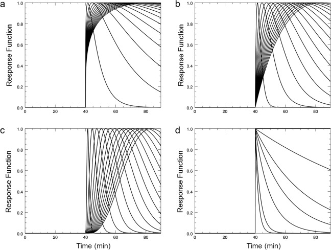
Response functions of lp‐ntPET to model transient dopamine release at t _d = 40 min. Gamma‐variate function with α equal to 0.25 (a), 1 (b), and 4 (c) and exponential function with β = [0, 0.01, 0.03, 0.05, 0.1, 0.3, 0.5] (d).

lp‐ntPET estimation process

The library of response functions h_i(t) are determined by selecting discrete parameter values (t _D, t _P, and α) [Eqs. (3a) and (3b)] over finite intervals. Basis function [B_i(t)] candidates are then created as the integral of the product of the TAC in the target region and each response function. Four explicit model parameters (R ₁, k ₂, k _2a, and γ) in Eq. (1) are estimated using weighted least squares with each candidate basis function. As the final output, one basis function B_i(t) is selected that yields the best fit to the PET data when compared with all other candidate basis functions.

Significance testing

After fitting data using the lp‐ntPET model, the F‐test is performed to test the goodness of fit of lp‐ntPET when compared with the simpler MRTM model using Eq. (4). The F‐test is appropriate for comparing the fits of “nested” models such as MRTM and lp‐ntPET. The null hypothesis is that there is no improvement in the fitting by including the time‐varying response term, B_i(t), that is unique to lp‐ntPET [Eqs. (1) and (2)].

$$F=\frac{\left(\frac{\mathrm{WRS}{\mathrm{S}}_{\mathrm{MRTM}}-\mathrm{WRS}{\mathrm{S}}_{\mathrm{l}\mathrm{p}-\mathrm{ntPET}}}{p_{\mathrm{l}\mathrm{p}-\mathrm{ntPET}}-{\mathrm{p}}_{\mathrm{MRTM}}}\right)}{\left(\frac{\mathrm{WRS}{\mathrm{S}}_{\mathrm{l}\mathrm{p}-\mathrm{ntPET}}}{\mathrm{n}-{\mathrm{p}}_{\mathrm{l}\mathrm{p}-\mathrm{ntPET}}}\right)},$$ (4)

where WRSS is the weighted residual sum of squares, p is the number of model parameters, and n is the number of data points in a TAC.

The details of the theory of lp‐ntPET have been described in a previous paper by Normandin et al. [2012].

Study Design

We chose a single scan design to detect the DA response to cigarette smoking. The radiotracer (¹¹C‐raclopride) was administered as a bolus‐plus‐constant infusion (B/I). The subject smoked two successive cigarettes (of their own brand) in the PET scanner beginning 45 min after the start of the PET scan. To validate our method's specificity for the smoking‐induced DA signal, a rest scan was obtained as well. The rest scan was performed on a separate day in the same way, with the same subject but without smoking.

Extension to Voxel‐Based lp‐ntPET Model

Because the lp‐ntPET model is a linear, basis function‐based method for fitting the dynamic PET data, it is practical to implement it as a voxel‐by‐voxel method. In this study, we have extended lp‐ntPET to voxel‐based lp‐ntPET. The resulting analysis process is composed of four main steps: preprocessing, modeling, statistical comparisons, and visualization.

Preprocessing

In the preprocessing step, a spatial smoothing filter is applied to the PET data. We used the highly constrained back‐projection (HYPR) spatial filter [Christian et al., 2010] to reduce spatial noise with the hope of preserving critical temporal information (i.e., temporal “edges”). The spatially filtered PET data is registered to a standard template space. Next, a reference tissue TAC is extracted. For ¹¹C‐raclopride data, we used the cerebellum as the reference region. Only voxels in precommissural striatal region were examined because (a) this region has sufficient signal to background contrast with ¹¹C‐raclopride and (b) it is the region of the brain that is implicated in drug addiction, craving, and reward.

Modeling

In the modeling step, the PET TAC at each individual voxel is fitted using both the lp‐ntPET model and MRTM. For lp‐ntPET fits, response functions are selected first. We used the following discrete set of parameter values for the gamma‐variate function for this ¹¹C‐raclopride smoking study. Three α values were 0.25, 1, and 4 for sharpness. Response start times (t _D) were set between (smoking time − 5 min) to (smoking time + 15 min) in increments of 1.5 min, which is one half the frame duration. Peak response times (t _P) were set between (t _D + 1.5 min) and (total scan time − 5 min) in increments of 1.5 min (Fig. 1a–c). In the case of smoking at 45 min, the lowest possible value of t _D was chosen to be 40 min to allow for DA response due to anticipation of smoking. We included pure exponential functions, $\mathit{h}\left(\mathit{t}\right)={\mathit{e}}^{-\mathit{\beta t}}$, in the response function library to allow for instantaneous increases in DA at individual voxels. The seven different preselected exponential time constants β for $e^{-\beta t}$ were 0, 0.01, 0.03, 0.05, 0.1, 0.3, and 0.5 (Fig. 1d). For a total scan time = 90 min, 300 response functions were generated. Fitting the lp‐ntPET model at each voxel produces not only images of the parameters (R ₁, k ₂, k _2a, and γ) but also a WRSS image (WRSS_lp‐ntPET). Fitting MRTM to voxelwise data yields estimates of only three parametric images (R ₁, k ₂, and k _2a) and a WRSS image (WRSS_MRTM).

Statistical comparison

The statistical comparison requires two steps.

F‐statistic

The F map was generated from the two WRSS maps by calculating the F‐statistic [Eq. (4)] at each voxel. The F‐statistic compares the WRSS_lp‐ntPET to the WRSS_MRTM, correcting for differences in degrees of freedom in the respective fits. For this test, we considered the number of lp‐ntPET model parameters to be seven. Four are explicit kinetic parameters [see Eq. (1)], and three are implicit gamma‐variate function parameters [Eq. (3a)]. When the response function is a simple exponential [Eq. (3b)], there are only two implicit parameters. Thresholding (P < 0.05) was performed based on degrees of freedom in the model fits. The threshold was the same at every voxel. The resulting binarized image after thresholding is called the “significance mask.”

Cluster‐size threshold

After the F‐test, we applied a cluster‐size threshold as a means of correcting for multiple comparisons. This idea has been advanced by Holmes et al. [1996]. Clusters are defined as non‐negative voxels in the significance mask that are connected with each other. Separate clusters were identified in a binarized 3D image using a blob coloring algorithm (Label_region function in IDL). Cluster size is determined by counting the number of voxels in the cluster. In our data, the number of separate clusters and their respective cluster sizes were determined in each significance mask following F‐statistic thresholding. Cluster‐size distributions that result entirely by chance were created by applying the entire lp‐ntPET analysis process to simulated 4D rest data (i.e., null data). Cluster‐size thresholds were set to exclude 99% of the clusters that were produced by chance through the lp‐ntPET analysis of simulated rest data. Only the largest 1% of clusters were retained. In the analysis of smoking data, all clusters were eliminated that were smaller than the predetermined cluster‐size threshold.

Visualization (4D DA movie)

For each voxel retained in the final significance mask, the estimated DA values over time [γh(t)] normalized by the estimated k _2a at each respective voxel was stored. These normalized DA images are four‐dimensional (4D). They represent the DA value at each time point for each voxel found to have a significant DA response to the stimulus. Color‐coded image series were created by applying a color lookup table to the normalized DA images. The color‐coded 4D images were overlaid on a static MR template for the corresponding brain slices to create “DA movies.”

Simulation

Generating 4D‐simulated PET phantom data

To help in selecting appropriate thresholds and to fully characterize our method, we simulated phantom data with a similar noise level to our real PET data. For simulated data, noiseless target and reference region TACs were first generated using the full ntPET model [Morris et al., 2005], which is a nonlinear model of tracer binding to a receptor in the presence of a time‐varying endogenous competitor.

Simulated rest data

For the simulated rest data, target region parameters were set to K ₁ = 0.0918 mL/(min g), k ₂ = 0.4484/min, k _on = 0.0282 mL/(pmol min), k _off = 0.1363 min⁻¹, B _max = 44 pmol/mL, F _v = 0.04 mL/mL, and $k_{\text{on}\hspace{0.17em}}^{\text{DA}\hspace{0.17em}}$ and $k_{\text{off}\hspace{0.17em}}^{\text{DA}\hspace{0.17em}}$ = 0 [Pappata et al., 2002]. A reference region was simulated by setting as $K_1^{\text{ref}\hspace{0.17em}}$ = 0.0918 mL/(min g) and $k_2^{\text{ref}\hspace{0.17em}}$ = 0.4484 min⁻¹. Each simulated dataset contains 1,004 TACs of 120 min of data with 3‐min frame duration to match our real PET data.

Simulated smoking data

Four versions of simulated smoking data were produced to represent a variety of weak to strong responses to a stimulus. Free endogenous DA (F ^DA) release in the form of a gamma‐variate function [Eq. (3a)] was applied to the full ntPET model. The F ^DA function was simulated with $k_{\text{on}\hspace{0.17em}}^{\text{DA}\hspace{0.17em}}$ = 0.25 mL/(pmol min), $k_{\text{off}\hspace{0.17em}}^{\text{DA}\hspace{0.17em}}$ = 25 min⁻¹, and basal DA level = 100 nM [Morris et al., 1995]. For the gamma‐variate function, t _D = 45 min, t _P = 50 min, α = 2, and peak DA levels (peak DA) = 150, 200, 300, and 800 nM.

Noise

Gaussian noise with zero mean and the following variance [Eq. (5)] were added to the ith time frame of the noiseless tissue TAC.

$$\sigma =\mu \times \left(\sqrt{\left(C_T(t_i)\times e^{-\lambda t_i}\right)/\Delta t_i}\right)\times e^{\lambda t_i}$$ (5)

The constant μ is the scaling factor that determines the noise level. λ is the decay constant for ¹¹C, and Δt_i is the ith frame length. For setting the constant μ to reflect our real data, we measured the average coefficient of variation (ratio between averaged noise variance and mean of the last 15 min of ¹¹C‐raclopride PET concentration) in two real PET rest datasets. To confirm the similarity of the noise level in simulations with the noise level in the data, F‐distributions after lp‐ntPET in both PET data and simulations were compared.

Making 4D phantom data

To create a 4D phantom, noisy simulated TACs were placed at each voxel in the dorsal striatal mask in template space. The dorsal striatum mask consisted of 1,004 voxels. Therefore, 1,004 noisy TACs were generated for each dataset. In total, 100 rest and 4 × 100 smoking datasets for different DA level were generated. Random noise was generated anew each time. Two different styles of smoking data were generated: (1) a smoking phantom was created with DA activation in every voxel of the dorsal striatum region, and (2) a second smoking phantom was created with DA activation only in clusters of different sizes each smaller than the striatum region.

Cluster‐size distribution as correction for multiple comparisons

lp‐ntPET was applied to 100 rest 4D phantoms. After thresholding the F map at each voxel (at P < 0.05), adjacent voxels in the significance mask were counted as a single cluster using the blob coloring algorithm based on six‐neighbor connectedness. The number of voxels of each cluster was counted to determine the cluster size. The histogram of cluster size was plotted for all 100 datasets. The cumulative probability density function was plotted to obtain the cluster threshold corresponding to the P < 0.01 level.

Sensitivity map

Sensitivity maps were created to estimate the true positive detection rate at each voxel in the simulated striatum. To create sensitivity maps, we started with 100 simulated smoking datasets. Each dataset was analyzed with lp‐ntPET, and a cluster‐size threshold was applied based on the cluster‐size distribution calculated above. The resulting 100 binary significance masks were summed to a single map representing the percent true positive rate at every voxel.

Bias of DA parameters

t _P, t _D, and peak DA were estimated using lp‐ntPET at each voxel in the smoking phantoms. Biases in the estimated parameters were calculated based on the analysis of phantom smoking datasets.

All simulations were implemented in Matlab (R2008b; MathWorks, Natick, MA) using modeling functions provided by the COMKAT library [Muzic and Cornelius, 2001] and using IDL 8.0 (Exelis Visual Information Solutions, Boulder, CO).

Experiments With Human Smokers

Subjects

All study procedures were approved by the Yale University Human Investigations Committee. Two male tobacco smokers (aged 20 and 48 years) were scanned. Subjects were abstinent from smoking for at least 2 h prior to their rest scan and at least 12 h prior to their smoking scan to increase craving for the cigarette. On arrival at the PET Center, subjects completed questionnaires to rate their smoking urges (QSU‐Brief) [Cox et al., 2001] and withdrawal symptoms (MNWS) [Hughes and Hatsukami, 1986]. Plasma cotinine and nicotine levels were assayed before scans to confirm compliance with abstinence on smoking days. Subjects were instructed to smoke at their normal pace during the PET scan. The order of smoking and rest was opposite between two subjects.

Data acquisition

Subjects received a 3T structural MRI on a different day from the PET scan days for use in aligning PET data to the template space. Typical acquisition parameters for the structural MRI were 3D MPRAGE MR pulse sequence with TE = 3.3 ms, flip angle = 7°; slice thickness = 1.0 mm, and 0.98 × 0.98 mm² pixels.

PET scans were acquired for 2 h (40 × 3 min) with B/I (K _bol = 105 min) of tracer in the HRRT PET scanner (Siemens/CTI, Knoxville, TN). Injected doses and specific activities of ¹¹C‐raclopride were 741 ± 29 MBq and 450 ± 189 MBq/nmol, respectively. The Vicra optical tracking system (Vicra, NDI Systems, Waterloo, Canada) was used to measure and record subject head movement during each scan. List‐mode dynamic data were reconstructed with all corrections (attenuation, normalization, scatter, randoms, dead time, and motion) using the MOLAR algorithm [Carson et al., 2003].

Data analysis

A spatial filter, HYPR [Christian et al., 2010], was applied with 3D box kernels (6 × 6 × 6 mm³) to all PET images in a frame‐by‐frame manner to reduce spatial noise without degrading the temporal information at every voxel.

PET data were aligned to each subject's MR data and then registered to the AAL MR template. Reference TACs were extracted from an AAL‐defined cerebellum. Following Mawlawi et al. [2001], we applied a mask of the precommissural striatum (ventral striatum, dorsal caudate, and dorsal putamen) to all the PET data in template space because this brain area is implicated in drug addiction.

For lp‐ntPET modeling, the same basis functions were used that were used in creation of the phantoms. A cluster‐size threshold of 17 voxels was applied based on the simulation result. Significance masks and DA curves in the significance masks from both the rest and smoking conditions were assessed.

RESULTS

Simulation

Simulated noisy rest data at the voxel level

Experimental and simulated TACs at the voxel level are shown in Figure 2. For illustration purposes, the data points in Figure 2a show a ¹¹C‐raclopride TAC taken from a single voxel in the ventral striatum during the rest scan of a smoker. The smooth curve in Figure 2a represents the fit of MRTM to the data points. The smooth curve in Figure 2b is a noiseless simulation using the complete ntPET model [Morris et al., 2005] with no DA activation (no deviation of DA from basal level). The data points in Figure 2b represent random noise (average coefficient of variation = 20%) added to the noiseless curve. The choice of 20% coefficient of variation is based on the analysis of ¹¹C‐raclopride scans performed on two different smokers at rest (not smoking). In those two subjects, the coefficients of variation in the PET data were 17.8% and 21.7%, respectively. Note the similarity in apparent noise level between the simulation and the real data.

Figure 2.

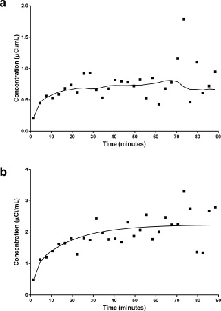
Single PET voxel rest data (a) with fitted curve using MRTM in ventral striatum region (solid line) and single voxel level‐simulated rest data (b) with true value (solid line).

The distributions of F values for both a simulated rest dataset and a real‐rest PET dataset are shown in Figure 3. Figure 3a shows the F‐distribution for the simulated dataset, and Figure 3b corresponds to the real data. Note the very close similarity of the two distributions. Taken together, Figures 2 and 3 suggest that the noise characteristics in our noisy simulations properly reflect the noise in our human [¹¹C]raclopride PET data.

Figure 3.

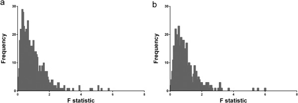
Distribution of F‐ratio based on (a) simulated rest data and (b) real‐rest PET data in human subject. F‐ratios are generated at each voxel in dorsal striatum by comparing the weighted residual sum of squares of the lp‐ntPET fit to that of the MRTM fit to the same TAC.

Cluster‐size distribution as a means of correcting for multiple comparison

The cluster‐size distribution from the lp‐ntPET analysis of 100 simulated rest datasets is shown in Figure 4 (gray bars). The solid curve represents the cumulative probability distribution, that is, the probability of finding a cluster of a given size or less. The cluster‐size threshold required to exclude 99% (P < 0.01) of all clusters from occurring by chance in an lp‐ntPET analysis of rest data is shown as a dotted vertical line at 15 voxels.

Figure 4.

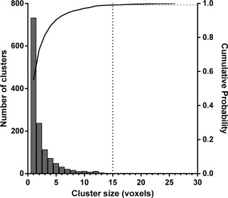
Cluster‐size distribution after thresholding F maps produced from the simulated rest data. Solid curve represents cumulative probability. Dotted vertical line shows where to set cluster‐size threshold to exclude 99% (P < 0.01) of clusters that will occur by chance in the lp‐ntPET analysis of rest data (no dopamine activation) based on 100 simulations of phantom images.

After eliminating clusters smaller than 15 voxels, we observed that 87/100 datasets had no remaining clusters in their final significance mask (Table 1). When we adjusted the cluster‐size threshold to 17 voxels, 90% of the significance masks were completely free of random clusters (Table 2). Thus, we can say that the likelihood of detecting clusters larger than 17 voxels by chance (i.e., the false positive rate) is less than or equal to 10%.

Table 1.

Probability of cluster size

Number of clusters bigger than 15 voxels	Number of datasets
0	87
1	12
2	1
Total	100

Table 2.

Probability of cluster size

Number of clusters bigger than 17 voxels	Number of datasets
0	90
1	9
2	1
Total	100

Simulated smoking data and sensitivity of voxelwise lp‐ntPET

The DA responses used to create simulated smoking data are shown in Figure 5a. The resulting noiseless TACs for each of the four different peak DA levels are shown in Figure 5a (inset). An example of single noisy simulated smoking TAC corresponding to a peak DA level of 200 is shown in Figure 5b.

Figure 5.

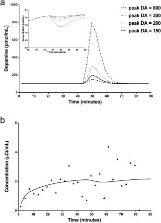
(a) Dopamine response with increasing peak height used to create simulated smoking data. Baseline DA level equals to 100 pmol/mL. Simulated TAC is decay‐corrected. (b) Single noisy simulated smoking TAC with peak DA level 200.

Every voxel in the dynamic phantom of smoking data contains a TAC similar to the noisy one shown in Figure 5b. A sensitivity map based on the lp‐ntPET analysis of a smoking phantom with peak DA level set to 200 (four coronal slices of striatum) is shown in the bottom row of Figure 6.

Figure 6.

Sensitivity map in whole dorsal striatum region at given uniform dopamine signal over 100 runs (peak DA = 200).

Sensitivity values at the edge of each slice are lower than those at the center. In addition, the first and last slices have low sensitivity when compared with the middle slices. A sensitivity map for a phantom containing multiple, isolated clusters of activation, each with peak DA level 200 but differing in size, is shown in Figure 7. The size of each cluster in the phantom is indicated on the slice at the left in the first row of the figure. The average sensitivity values as a function of both cluster size and peak DA level are summarized in Table 3. No significant clusters were found in the right caudate, which contained no true DA responses. The dependence of sensitivity on cluster size and peak DA level is plotted as a surface in Figure 8.

Figure 7.

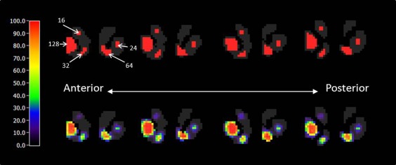
Four‐slice phantom containing clusters of different sizes (top) and sensitivity map (peak DA = 200; bottom). Number with arrow indicates the number of voxels contained in each cluster. Voxel size is 2 × 2 × 2 mm³.

Table 3.

Sensitivity table

Peak DA level (pmol/mL)	Cluster size (number of voxels)
	16	24	32	64	128
150	2.5%	8.6%	14.4%	25.4%	35.8%
200	13.6%	32.5%	48%	68.7%	80.9%
300	51.1%	86.4%	84.2%	94.4%	97.5%
800	98.9%	100%	99.3%	100%	99.8%

1 voxel = 2 × 2 × 2 mm³; baseline DA level equals to 100 pmol/mL. Numbers represent sensitivity (%) to the presence of dopamine activation.

Figure 8.

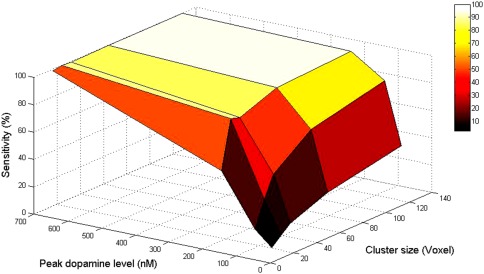
Sensitivity (ability to recover true DA activation) as a function of peak dopamine level and cluster size. Voxel size is 2 × 2 × 2 mm³.

Bias of DA parameters in simulated smoking data

The means and standard deviations of estimated DA parameters (response start time t _D, peak response time t _P, and peak DA level) from the analysis of multiple versions of the smoking phantom with clusters of activation (see the top row of Fig. 7) are shown in Figure 9.

Figure 9.

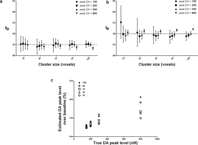
Bias of dopamine parameters for different dopamine levels.

The dotted lines in Figure 9a,b represent the true values of the parameters. With the exception of the very smallest cluster, the mean estimated values of t _D and t _P at peak DA levels of 150, 200, and 300 are very close to the true values (Fig. 9a,b). Note that the smallest cluster is below the cluster‐size threshold. At peak DA level 800, the bias in t _D is slightly negative (underestimation). t _P was slightly overestimated for high peak DA level. However, even these biases were less than 2 min. The error bars in Figure 9a,b indicate that the variation in the estimates of t _D and t _P decreased as cluster size increased (temporal precision improves with cluster size). At peak DA level 800, however, peak DA levels are severely underestimated as shown in Figure 9c. At lower peak DA levels (150, 200, and 300), we find a linear relationship between estimated and true peak DA level.

PET Experiments With a Human Smoker

Significance mask for smoke and rest conditions

Final significance masks for smoking and rest conditions are shown in Figure 10 for two different smokers. Clusters larger than 17 voxels were detected in the smoking scans of both smokers, but not in their rest scans (second and fourth rows of Fig. 10). Caudate was found to contain significant clusters of activation in both subjects. Significant voxels were also detected in ventral striatum and in the putamen region in one subject (third row of Fig. 10).

Figure 10.

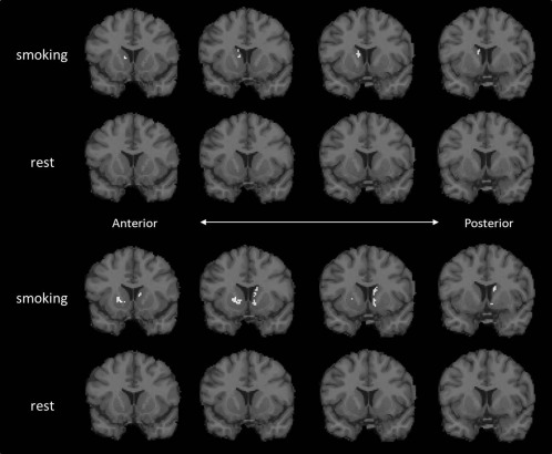
Significant voxels detected in PET data for two different smokers at rest and during smoking (top and bottom).

DA movies (curves) for smoking scans

DA response curves for each voxel in the three clusters isolated from the second subject's smoking data are plotted in Figure 11. The three different clusters are marked with different colors (green: ventral striatum; orange: putamen; and red: caudate). The mean ± one standard deviation of the DA responses in each cluster are shown in Figure 12. Peak times of the mean curves were 52.5 min for ventral striatum and putamen and 58.5 min for caudate.

Figure 11.

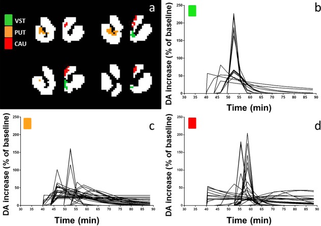
DA response curves for each voxel in each significant cluster (b–d) in four different slices through the striatum (a) in one subject's smoking scan (VST, ventral striatum; PUT, putamen; CAU, caudate).

Figure 12.

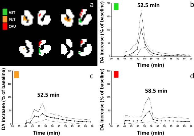
Average DA curves in the significant clusters of one subject's smoking scan. Solid curves represent the mean of the data curves in Figure 11, and the dotted curves represent the mean + SD and the mean − SD, respectively.

The multislice, multicondition DA movies for two smokers are available in Supporting Information. Each DA movie displays the frame‐by‐frame DA level relative to the baseline DA level. All slices of precommissural ventral striatum are displayed simultaneously for rest and smoking conditions. Neither subject showed any significant voxels in the rest state. In contrast to the second subject, the first subject showed a DA response only in the right caudate during the smoking scan. The DA peak time for the cluster of activation in the caudate was 55.5 min.

DISCUSSION

Visualization of DA Movies

We have extended a new linearized mathematical technique [Normandin et al., 2012], lp‐ntPET, to be applicable at the voxel level in order to capture brief, localized DA events embedded within PET data. A key endpoint of our work is a DA movie (in contrast to a movie of PET activity) resulting from the estimation of transient DA changes at each voxel in the dynamic data. The DA movie is a 4D output. Thus, due consideration must be paid to how it can best be visualized. In general, the movie results from the color coding of DA values, which represent fractional increases in DA above baseline. Without any further processing, associated voxels that peak at different (fractional) levels will be shown in different colors and thus may appear to belong to distinct populations (clusters). Alternatively, DA values at each voxel could be normalized by their individual peak values. If so, then voxels that peak at the same time would be displayed in the same color at that peak time. Thus, the similarities of two voxels would be more apparent. For the moment, we have chosen to display the DA movies using the former scheme, but going forward, as we seek to capitalize on the pattern recognition powers of the human observer, we may choose to follow the latter—or yet another—visualization strategy. In any case, revealing the temporal patterns of DA activation in local brain regions is our goal and this work is motivated, in part, by the theory that the speed of DA release in response to drugs encodes a drug's addiction liability [Volkow and Swanson, 2003].

Sensitivity of lp‐ntPET

In this study, four DA signals of different magnitude were simulated to consider a wide range of activations. In previous microdialysis studies, administration of nicotine in doses relevant to smoking produced 200% [Pontieri et al., 1996] and 250% [Domino and Tsukada, 2009] increases in extracellular DA above baseline in the striatum of rats and monkeys, respectively. Cocaine and amphetamine can increase DA anywhere from 250 to 1,000% in the rat striatum [Carboni et al., 2001]. Our sensitivity maps (Figs. 6 and 7) and related surface plot (Fig. 8) show that our ability to detect activation is not simply a matter of magnitude but a joint function of magnitude and spatial extent. Based on our sensitivity maps, we assert that lp‐ntPET can detect moderate DA responses (those that peak at two times the baseline level) 80–90% of the time if the DA response occurs uniformly in a large portion of the striatum (Fig. 6). On the other hand, if the DA response occurs in a very small area (i.e., 24 voxels × 8 mm³; approximately one‐tenth of the ventral striatum volume), the signal must peak at three times baseline or higher for signal detection to reach 80% sensitivity.

Timing Parameters Are Minimally Biased

lp‐ntPET showed good precision in estimating timing parameters (t _D and t _P) of the DA responses at the voxel level (Fig. 9). This finding was consistent with the previous evaluation of ROI‐based lp‐ntPET [Normandin et al., 2012]. Good temporal resolution would be important for sequencing activation events (involving the same neurotransmitter system) that occur in different brain areas at different times. In our sample PET data from an ongoing study of cigarette smoking, we observed that the DA response peaked at 52.5 min (7.5 min after the start of smoking) in clusters in the ventral striatum and dorsal putamen but at 58.5 min (13.5 min after the start of smoking) in a cluster in the dorsal caudate (Fig. 12). Each of the significant clusters identified with voxelwise lp‐ntPET analysis of our smoking data were larger than 17 voxels. On the basis of our simulation studies, the standard deviations of t _D and t _P for small to moderate DA responses most relevant to smoking (DA peaks between two and three times baseline) were both less than 4 min in small clusters (16 voxels; Fig. 9). Thus, we feel confident in claiming that the average responses identified in clusters in the ventral striatum and putamen of the subjected depicted in Figures 10 (bottom), 11, and 12 were both distinct temporally from, and earlier than, the (average) temporal response in the caudate. We hope to use this type of temporal resolution to explore the nature of the DA responses to addictive substances and the effect of treatments. It may also be possible to improve the temporal resolution of our estimates by reducing the duration of PET time frames below the 3‐min bins used in our sample studies here. Naturally, there is an ever‐present trade‐off between shorter time bins and higher noise that must be heeded.

Cluster‐Size Threshold to Correct for Multiple Comparisons

We are applying a statistical test (DA present or not) at many voxels. Therefore, we must correct for multiple comparisons. Without such a correction, the sheer number of comparisons will lead to a considerable number of false positive findings. One common approach to this problem is the family‐wise error correction method, for example, Bonferroni correction [Hochberg and Tamhane, 1987]. In brief, Bonferroni method uses a corrected P value by dividing the desired P value by the number of comparisons (voxels). However, this method can be overly conservative. When Bonferroni correction was applied to our data, no significant voxels were found in our experimental PET data. Instead, we chose the cluster‐size threshold approach to retain adequate sensitivity to activation while still eliminating false positives. The idea of cluster‐size inference dates back at least to work in 1993 by Poline and Mazoyer [1993] and Roland et al. [1993]. Shortly thereafter, Votaw and Li [1995] used the technique to detect regions of activation in difference images. In their study, the significance level was selected to permit no more than one false positive cluster per every 20 brains (i.e., “global” P < 0.05). In the same way, we set our desired global level of significance as P < 0.1. It is satisfying to note that when we applied our algorithm to our simulated image sequences, we did not find any false positive clusters in the background areas in which there was no DA response (e.g., right caudate in Fig. 7). In our real PET data, in the rest condition, no significant clusters were found.

LSSRM Versus lp‐ntPET

LSSRM is another advanced imaging technique that is aimed at detecting the effect of time‐varying neurotransmitter release in PET brain images. This technique is based on an enhanced kinetic model that allows for time‐dependent changes in the apparent efflux rate parameter [i.e., k _2a in Eq. (2)]. However, the configuration of LSSRM [fixed DA response shape (exponential), fixed take‐off time for activation (t _D = task start time)] limits the application of LSSRM to certain stimuli that elicit a DA response at a known time and are instantaneously maximal. In contrast, lp‐ntPET incorporates flexibility into the selection of the temporal aspects of the DA response. This flexibility is conveyed through the use of a predefined library of response functions that produce a corresponding library of basis functions to describe the effect of the neurotransmitter activation on the PET curve. To create a reasonable library of possible responses to smoking, we included a large set of gamma‐variate functions and exponential functions in the library. In our analysis of our real smoking study data, we found that the model returned DA responses that peaked between 8 and 14 min after smoking and disappeared ∼10 min later (see Fig. 12). LSSRM cannot differentiate responses with different delay times or peak times and thus may not be equipped to adequately fit data from smoking or from studies of other similar behaviors.

As with LSSRM, lp‐ntPET does not have an explicit term for change in blood flow. However, we remind the reader that in the previous simulation study by Normandin et al. [2012], the changes imposed on K ₁ and k ₂ (the two parameters that depend on flow in the model used to simulate the data) in the middle of the scan do not appreciably alter the estimates of DA parameters.

Computation Time

Although the implementation of lp‐ntPET dictates that it must perform one fit for every predefined response function in its library, these are linear fits and the overall computation time is quite small. In our analysis of the PET data from our smoking study, we used a library with ∼300 response functions. The analysis of the entire dorsal striatal region (about 1,000 TACs corresponding to 1,000 voxels) took less than 1.2 min on a moderately powered PC (Intel Core2 Duo CPU 2.93GHz with 3.5 GB RAM) including some prefiltering of the images. This computational load is certainly manageable for routine analysis of dynamic images—even if a different tracer was used that demanded analysis of the whole brain.

Possible Uses and Advantages of Voxelwise lp‐ntPET

In the recent study by Sullivan et al. [2013], a previously unexplained discrepancy between two early smoking studies [Brody et al., 2004, 2006] was explained in terms of the severe dependence of ΔBP, as a measure of DA release, on the size (duration) of the PET data window. This dependence—caused by violation of the assumption of steady DA levels—makes the comparison of different studies using ΔBP and different paradigms to characterize the response to smoking almost impossible. It also supports the idea that the DA response to cigarette smoking is not long‐lasting. Indeed, animal studies using microdialysis have shown that the DA response to nicotine is brief [Di Chiara and Imperato, 1988; Maisonneuve et al., 1997]. lp‐ntPET can capture brief DA activation, whereas conventional methods cannot. In addition, recent studies have found highly localized clusters of DA activation in the cortex in response to a reward‐learning task [van Eimeren et al., 2013] and a mathematical task designed to induce stress [Lataster et al., 2014; Vrieze et al., 2013]. As we have shown here, voxelwise lp‐ntPET can be used to detect short‐lived responses of the DA system occurring in small brain areas (small clusters of voxels). Thus, we believe that lp‐ntPET offers two possible advantages over other methods. (1) In circumstances, such as the study of addictive liability of drugs or the effect of treatment for addiction, where the precise timing of DA release may be at issue, the lp‐ntPET model can estimate (and differentiate) the timings of the local DA responses. Here, one could imagine monitoring the speed of DA release regionally, with the progression of dependence or before and after treatment for dependence. (2) More generally, in the use of PET to study responses to various behaviors and behavioral tasks that induce local and short‐lasting DA changes, lp‐ntPET will, by virtue of its time‐varying terms, be a better model than conventional ones for the effect of DA release on dynamic PET data. The use of a more appropriate model may yield significant findings where the conventional ones would not.

CONCLUSION

In this study, lp‐ntPET has been extended to the voxel level to create neurotransmitter release movies. These movies reveal interesting and previously unobserved localized, transient changes in DA levels in the striatum in response to cigarette smoking. The analysis of realistic simulations showed that the sensitivity to rapid DA changes that are relevant for smoking is greater than 80%. Biases in the estimates of timing parameters (DA response start time, peak response time) were close to 0. The false positive rate, caused by the large number of voxels examined, and hence large number of statistical tests performed, was well controlled using the F‐test (proposed in the original algorithm) and a cluster‐size threshold (introduced specifically for voxelwise lp‐ntPET). We presented novel DA movies of the response to smoking cigarettes in the PET scanner. The movies revealed the possibility of distinct timing of DA changes in different subregions of the striatum. These spatiotemporal patterns of DA release could serve as novel markers of disease (e.g., dependence), additive liability of drugs of abuse, or signatures of treatment efficacy.

Supporting information

Supplementary Information Figure 1.

Supplementary Information Figure 2.

Supplementary Information Figure 3.

Supplementary Information Figure 4.

REFERENCES

- Alpert NM, Badgaiyan RD, Livni E, Fischman AJ (2003): A novel method for noninvasive detection of neuromodulatory changes in specific neurotransmitter systems. Neuroimage 19:1049–1060. [DOI] [PubMed] [Google Scholar]
- Brody AL, Olmstead RE, London ED, Farahi J, Meyer JH, Grossman P, Lee GS, Huang J, Hahn EL, Mandelkern MA (2004): Smoking‐induced ventral striatum dopamine release. Am J Psychiatry 161:1211–1218. [DOI] [PubMed] [Google Scholar]
- Brody AL, Mandelkern MA, Olmstead RE, Scheibal D, Hahn E, Shiraga S, Zamora‐Paja E, Farahi J, Saxena S, London ED, McCracken JT (2006): Gene variants of brain dopamine pathways and smoking‐induced dopamine release in the ventral caudate/nucleus accumbens. Arch Gen Psychiatry 63:808–816. [DOI] [PMC free article] [PubMed] [Google Scholar]
- Carboni E, Spielewoy C, Vacca C, Nosten‐Bertrand M, Giros B, Di Chiara G (2001): Cocaine and amphetamine increase extracellular dopamine in the nucleus accumbens of mice lacking the dopamine transporter gene. J Neurosci 21:RC141:1–4. [DOI] [PMC free article] [PubMed] [Google Scholar]
- Carson RE, Barker WC, Liow JS, Johnson CA (2003): Design of a motion‐compensation OSEM list‐mode algorithm for resolution‐recovery reconstruction for the HRRT In: IEEE Nuclear Science Symposium Conference Record, IEEE, Portland, OR, Vol. 1–5 pp. 3281–3285. [Google Scholar]
- Christian BT, Vandehey NT, Floberg JM, Mistretta CA (2010): Dynamic PET denoising with HYPR processing. J Nucl Med 51:1147–1154. [DOI] [PMC free article] [PubMed] [Google Scholar]
- Constantinescu CC, Yoder KK, Kareken DA, Bouman CA, O'Connor SJ, Normandin MD, Morris ED (2008): Estimation from PET data of transient changes in dopamine concentration induced by alcohol: Support for a non‐parametric signal estimation method. Phys Med Biol 53:1353–1367. [DOI] [PubMed] [Google Scholar]
- Cox LS, Tiffany ST, Christen AG (2001): Evaluation of the brief questionnaire of smoking urges (QSU‐brief) in laboratory and clinical settings. Nicotine Tob Res 3:7–16. [DOI] [PubMed] [Google Scholar]
- Di Chiara G, Imperato A (1988): Drugs abused by humans preferentially increase synaptic dopamine concentrations in the mesolimbic system of freely moving rats. Proc Natl Acad Sci USA 85:5274–5278. [DOI] [PMC free article] [PubMed] [Google Scholar]
- Domino EF, Tsukada H (2009): Nicotine sensitization of monkey striatal dopamine release. Eur J Pharmacol 607:91–95. [DOI] [PubMed] [Google Scholar]
- Endres CJ, Kolachana BS, Saunders RC, Su T, Weinberger D, Breier A, Eckelman WC, Carson RE (1997): Kinetic modeling of [11C]raclopride: Combined PET‐microdialysis studies. J Cereb Blood Flow Metab 17:932–942. [DOI] [PubMed] [Google Scholar]
- Gunn RN, Lammertsma AA, Hume SP, Cunningham VJ (1997): Parametric imaging of ligand‐receptor binding in PET using a simplified reference region model. Neuroimage 6:279–287. [DOI] [PubMed] [Google Scholar]
- Hochberg Y, Tamhane AC. 1987. Multiple Comparison Procedures. Wiley, New York: 450 p. [Google Scholar]
- Holmes AP, Blair RC, Watson JD, Ford I (1996): Nonparametric analysis of statistic images from functional mapping experiments. J Cereb Blood Flow Metab 16:7–22. [DOI] [PubMed] [Google Scholar]
- Hughes JR, Hatsukami D (1986): Signs and symptoms of tobacco withdrawal. Arch Gen Psychiatry 43:289–294. [DOI] [PubMed] [Google Scholar]
- Ichise M, Liow JS, Lu JQ, Takano A, Model K, Toyama H, Suhara T, Suzuki K, Innis RB, Carson RE (2003): Linearized reference tissue parametric imaging methods: Application to [11C]DASB positron emission tomography studies of the serotonin transporter in human brain. J Cereb Blood Flow Metab 23:1096–1112. [DOI] [PubMed] [Google Scholar]
- Lammertsma AA, Hume SP (1996): Simplified reference tissue model for PET receptor studies. Neuroimage 4 (Part 1):153–158. [DOI] [PubMed] [Google Scholar]
- Lataster J, Collip D, Ceccarini J, Hernaus D, Haas D, Booij L, van Os J, Pruessner J, Van Laere K, Myin‐Germeys I (2014): Familial liability to psychosis is associated with attenuated dopamine stress signaling in ventromedial prefrontal cortex. Schizophr Bull 40:66–77. [DOI] [PMC free article] [PubMed] [Google Scholar]
- Logan J, Dewey SL, Wolf AP, Fowler JS, Brodie JD, Angrist B, Volkow ND, Gatley SJ (1991): Effects of endogenous dopamine on measures of [18F]N‐methylspiroperidol binding in the basal ganglia: Comparison of simulations and experimental results from PET studies in baboons. Synapse 9:195–207. [DOI] [PubMed] [Google Scholar]
- Maisonneuve IM, Mann GL, Deibel CR, Glick SD (1997): Ibogaine and the dopaminergic response to nicotine. Psychopharmacology (Berl) 129:249–256. [DOI] [PubMed] [Google Scholar]
- Mawlawi O, Martinez D, Slifstein M, Broft A, Chatterjee R, Hwang DR, Huang Y, Simpson N, Ngo K, Van Heertum R, Laruelle M (2001): Imaging human mesolimbic dopamine transmission with positron emission tomography. I. Accuracy and precision of D(2) receptor parameter measurements in ventral striatum. J Cereb Blood Flow Metab 21:1034–1057. [DOI] [PubMed] [Google Scholar]
- Morris ED, Fisher RE, Alpert NM, Rauch SL, Fischman AJ (1995): In vivo imaging of neuromodulation using positron emission tomography: Optimal ligand characteristics and task length for detection of activation. Hum Brain Mapp 3:35–55. [Google Scholar]
- Morris ED, Yoder KK, Wang C, Normandin MD, Zheng QH, Mock B, Muzic RF Jr, Froehlich JC (2005): ntPET: A new application of PET imaging for characterizing the kinetics of endogenous neurotransmitter release. Mol Imaging 4:473–489. [DOI] [PubMed] [Google Scholar]
- Morris ED, Normandin MD, Schiffer WK (2008): Initial comparison of ntPET with microdialysis measurements of methamphetamine‐induced dopamine release in rats: Support for estimation of dopamine curves from PET data. Mol Imaging Biol 10:67–73. [DOI] [PubMed] [Google Scholar]
- Morris ED, Kim SJ, Sullivan JM, Wang S, Normandin MD, Constantinescu CC, Cosgrove KP (2013): Creating dynamic images of short‐lived dopamine fluctuations with lp‐ntPET: Dopamine movies of cigarette smoking. J Vis Exp. 78. [DOI] [PMC free article] [PubMed] [Google Scholar]
- Muzic RF Jr, Cornelius S (2001): COMKAT: Compartment model kinetic analysis tool. J Nucl Med 42:636–645. [PubMed] [Google Scholar]
- Normandin MD, Morris ED (2008): Estimating neurotransmitter kinetics with ntPET: A simulation study of temporal precision and effects of biased data Neuroimage 39:1162–1179. [DOI] [PMC free article] [PubMed] [Google Scholar]
- Normandin MD, Schiffer WK, Morris ED (2012): A linear model for estimation of neurotransmitter response profiles from dynamic PET data. Neuroimage 59:2689–2699. [DOI] [PMC free article] [PubMed] [Google Scholar]
- Pappata S, Dehaene S, Poline JB, Gregoire MC, Jobert A, Delforge J, Frouin V, Bottlaender M, Dolle F, Di Giamberardino L, and others (2002): In vivo detection of striatal dopamine release during reward: A PET study with [(11)C]raclopride and a single dynamic scan approach. Neuroimage 16:1015–1027. [DOI] [PubMed] [Google Scholar]
- Poline JB, Mazoyer BM (1993): Analysis of individual positron emission tomography activation maps by detection of high signal‐to‐noise‐ratio pixel clusters. J Cereb Blood Flow Metab 13:425–437. [DOI] [PubMed] [Google Scholar]
- Pontieri FE, Tanda G, Orzi F, Di Chiara G (1996): Effects of nicotine on the nucleus accumbens and similarity to those of addictive drugs. Nature 382:255–257. [DOI] [PubMed] [Google Scholar]
- Roland PE, Levin B, Kawashima R, Åkerman S (1993): Three‐dimensional analysis of clustered voxels in 15O‐butanol brain activation images. Hum Brain Mapp 1:3–19. [Google Scholar]
- Sullivan JD, Kim S, Cosgrove KP, Morris ED (2013): Limitations of SRTM, Logan graphical method, and equilibrium analysis for measuring transient dopamine release with [11C]raclopride PET. Am J Nucl Med Mol Imaging 3:247–260. [PMC free article] [PubMed] [Google Scholar]
- van Eimeren T, Ko JH, Pellechia G, Cho SS, Houle S, Strafella AP (2013): Prefrontal D2‐receptor stimulation mediates flexible adaptation of economic preference hierarchies. Hum Brain Mapp 34:226–232. [DOI] [PMC free article] [PubMed] [Google Scholar]
- Volkow ND, Swanson JM (2003): Variables that affect the clinical use and abuse of methylphenidate in the treatment of ADHD. Am J Psychiatry 160:1909–1918. [DOI] [PubMed] [Google Scholar]
- Votaw JR, Li HH (1995): Analysis of PET neurofunctional mapping studies. J Cereb Blood Flow Metab 15:492–504. [DOI] [PubMed] [Google Scholar]
- Vrieze E, Ceccarini J, Pizzagalli DA, Bormans G, Vandenbulcke M, Demyttenaere K, Van Laere K, Claes S (2013): Measuring extrastriatal dopamine release during a reward learning task. Hum Brain Mapp 34:575–586. [DOI] [PMC free article] [PubMed] [Google Scholar]
Associated Data
This section collects any data citations, data availability statements, or supplementary materials included in this article.
Supplementary Materials