Connecting micro dynamics and population distributions in system dynamics models

Abstract

Researchers use system dynamics models to capture the mean behavior of groups of indistinguishable population elements (e.g., people) aggregated in stock variables. Yet, many modeling problems require capturing the heterogeneity across elements with respect to some attribute(s) (e.g., body weight). This paper presents a new method to connect the micro-level dynamics associated with elements in a population with the macro-level population distribution along an attribute of interest without the need to explicitly model every element. We apply the proposed method to model the distribution of Body Mass Index and its changes over time in a sample population of American women obtained from the U.S. National Health and Nutrition Examination Survey. Comparing the results with those obtained from an individual-based model that captures the same phenomena shows that our proposed method delivers accurate results with less computation than the individual-based model.

Introduction

When modeling a population of elements (e.g., people, tasks, widgets) that are heterogeneous with respect to a particular attribute (e.g., body weight, skill level, quality), system dynamics researchers tend to focus on capturing the mean of the attribute of the population aggregated in stock variables. However, many modeling problems require researchers to capture the heterogeneity and variation of attributes across the population elements (Osgood 2004; Osgood 2009). For example, in a study that aims to evaluate the effect of a weight loss intervention on a population, we may be interested in knowing how the intervention impacts people with different weights or Body Mass Index (BMI)¹ levels, because of the different health risks across the span of BMI (e.g. people with very high BMI are at significant risk for diabetes). Similarly, we may be interested in how software developers with different skill levels have different outputs as opposed to looking at the output associated with average skill level of developers in a company; how students with different intelligence levels have different academic performance; how members of social networks with different number of network connections change the dynamics of the network; how athletes with different ages have different performance levels; and how different levels of health indicators (e.g., cholesterol and blood pressure) can lead to different health outcomes associated with people in a population.

In all these scenarios, the heterogeneity of the population with respect to its attribute of interest is likely to have a strong impact on the dynamics under study. More generally, many modeling problems need to capture the distribution of the characteristics of interest in a population of elements and not only the mean of those characteristics, typically, because either the impact of the average of the attribute on system evolution is not obvious due to non-linearity, or we care about extreme cases in population represented by tails of the distribution. Using our example of a high tech firm, we might expect software developers with high levels of skill to show much higher productivity, or in the example of health indicators, that individuals with high BMI are prone to more severe health risks.

Researchers who need to explicitly capture such variations across the population elements generally utilize aging chains. In this approach, the elements are broken into different population groups based on their attribute value and are represented by different stocks. These fundamental stocks are then strung together to form the aging chain. Aging chains have been used for tracking the characteristics of a population (Sterman 2000; Eberlein and Thompson 2013), tracking the experience and promotion chain of employees (Snabe 2006; Größler and Zock 2010), and tracking the aging of equipment in a company (Schwarz and Maybaun 2004).

Aging chains have a simple conceptual structure and can easily be implemented. However, simple aging chains are best used for capturing characteristics which do not influence the propensity of an element to move across different groups. Thus, the movement of an element from one stock to another is a fraction independent of the attributes based on which we have divided the stocks in the chain. A common example is the use of aging chains to capture aging of a population. Here each element in each stock has a constant rate of movement to the next stock which can be directly determined based on the average duration of stay in that stock and does not depend on the age of the people in that stock.

However, in many real-world problems the movement of population elements across different percentiles on the distribution of an attribute of interest is a function of the location of an element on that distribution. Again using our examples, the current skill of employees influences their skill acquisition rate, the current number of links in a social network influences the rate of link acquisition, and the current weight of an individual influences the rate of weight gain and loss due to the effect of current weight on his or her energy intake and expenditure.

Currently, where the propensity of each element to move from one population group to another is a function of the characteristic by which the groups are specified, modelers formulate an aggregate function that controls the transition rates from each group to another. These rates are formulated without a clear mapping into the micro dynamics of population elements that generate those movements. For example, in modeling obesity, Homer and colleagues (2006) captured the movement of individuals from one population group, representing a specific BMI range, to another group using such aggregate functions.

The challenge with the current practice is that we don’t have any solid way to formulate the aggregate flow based on the physics of the problem. While the literature on the element we model, such as human weight gain and loss, can provides some fundamental mechanisms at the micro level, formulating the macro rates remains rather ad hoc and thus difficult to establish without calibration. Moreover, even when these macro rates can be calibrated to empirical data, doing so often sheds little light on how these rates would change in the event of interventions for which there is sparse empirical data, such as nutrition or physical-activity based interventions in the case of obesity.

Alternatively, the impact of such interventions or other changes can be studied via a microlevel model that captures the underlying mechanism at the individual level, e.g., how diet changes an individual’s energy intake. Agent-based model (ABM) architectures are popular for capturing the micro mechanisms directly (Rahmandad and Sabounchi 2011). However, applying this approach to large populations introduces a computational burden (Rahmandad and Sterman 2008). This computational expense may reduce the ability to conduct adequate calibration and sensitivity analysis. ABM architectures may also hide, within the complexity of agent interactions, the feedback mechanisms key to dynamics of interest.

The goal of this paper is to provide a consistent method for connecting micro-dynamics and macro distributional outcomes without using detailed agent-based models. Specifically, this research offers a solution for problems with the following characteristics:

• We model the dynamics of the distribution of a population of elements along attribute d (e.g., body weight, skill, social capital, defectiveness).

• We have a mechanism-based model at the element² level that captures this attribute, e.g., a model of weight gain and loss for individuals, a model of individual skill acquisition, a model for social capital growth of individuals, or a model of the propensity to accumulate defects for task elements.

• The individual-level mechanisms controlling the movement of the population elements along attribute d are functions of d itself. For example, the weight gain/loss of individuals depends on their current weight, since the energy expenditure of individuals depends on their weight in the forms of fat mass and fat free mass; skill acquisition rate in employees depends on their current skill level due to diminishing return on skill acquisition; and current number of links on a social network increases the rate by which individuals can meet others, thus increasing the rate of link acquisition.

After describing the proposed method, we model the BMI distribution associated with a sample of female adults and show how the distribution of BMI of this population will change due to a change in the energy intake. To capture the micro-level mechanism associated with weight gain and loss in individuals, we use a well-established model for human metabolism and body weight change (Hall, Guo et al. 2009). For validation, we compare and contrast our method to the benchmark results generated by an individual-based model of the same phenomenon.

The remainder of this paper is organized as follows. First, we explain the method and its rationale in detail. Next we describe the experimental setup regarding the application of the developed method to an empirical dataset. Then we examine the results. Lastly, we discuss limitations and areas for future research.

Methods

We consider a system that includes a population of n elements (e.g., people, tasks), each of which exhibits some values along attribute d (e.g., body weight, skill, defects). We disaggregate this population within several stocks based on their attribute values. For the general case of continuous attributes such as BMI, each stock contains members of the population whose attribute values fall within a specific range of the attribute of interest, e.g., a stock containing people whose BMI is between 25 and 28, another for BMI between 28 and 30, and so on. Population members who change their attribute values (e.g., lose or gain weight, acquire some skills, accumulate defects) contribute in flows between adjacent stocks of sub-populations (macro population groups).

To capture the transition rates between the macro population groups, we first allocate a representative individual to each group. These representative individuals characterize a typical individual in each sub-population (stock). We then find the macro-level transition rates between the sub-population groups based on the individual-level (micro-level) mechanisms that regulate the representative individuals’ attribute, by considering the representative individual in each group as moving on attribute d based on the micro-level dynamics without allowing the simulated representative individual to change its characteristic; accordingly, we estimate the rates of change for that individual’s sub-population to approximate the flow rate from the individual’s present stock to the adjacent stock. The process can be operationalized in the following four steps.

Step 1: Decide on the divisions needed along attribute d for disaggregating the population into sub-groups (macro population groups)

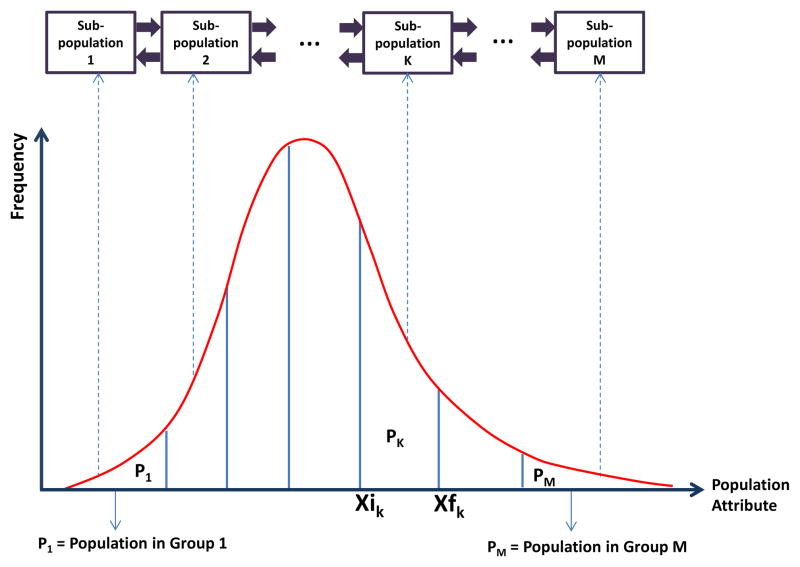
At this step, the domain of attribute of interest, d, is divided into several mutually exclusive intervals covering the full range of d represented by distinct consecutive stocks. This step is identical to devising stocks for an aging chain. Each one of these stocks now holds a sub-group of population whose attribute values fall within the attribute range associated with that stock. Figure 1 shows the distribution of an attribute in a population disaggregated into M distinct sub-groups, where P_k represents frequency of population elements in group k and Xi_k and Xf_k represent the initial and final values of the attribute interval associated with population group k, respectively. Note that in any two adjacent groups k and k+1, we have Xf_k = Xi_k+1.

Figure 1.

Disaggregation of population into macro population groups

We use the “subscripting” feature of Vensim^™ as a convenient way for disaggregating the population into distinct stocks according to their attribute range; most simulation packages have similar capabilities. Let subscript G (g₁, g₂, …, g_M) represent the vector of M stocks each representing a sub-population. Note that the subscripting process is conceptually equivalent to using M explicit stocks in the model and only simplifies the mechanics of implementation.

Step 2: Estimate the initial distribution of population elements along attribute d

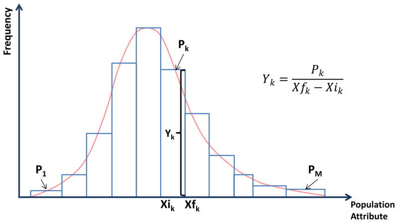
Initialize the model with values for the sup-population stocks and quantify the initial shape of the distribution. Estimate the stocks’ initial values directly from the known initial distribution of population along attribute d as represented by P_k. To specify the shape of the distribution, assume that individuals in each interval on attribute d are uniformly distributed along the interval range (Figure 2). Knowing the range of attribute values corresponding to each sub-population (stock) k (i.e., Xi_k and Xf_k), as well as the initial population associated with that group (P_k), calculate the height of the vertical bar associated with sub-population group k (Y_k), and use it to specify the shape of the distribution:

$$Y_k=\frac{P_k}{{Xf}_k-{Xi}_k}$$ (1)

Figure 2.

Estimating distribution of population individuals along attribute d

Note that choosing finer ranges for attribute values associated with each sub-population produces a better estimate of the true distribution of population along that attribute, but that increase in the precision comes at the cost of increasing the computational complexity of the model linearly with M.

Finally, to connect the individual-level dynamics to the population distribution, allocate a representative individual to each sub-population group. The representative individual of each group represents a typical individual in that group with respect to the attribute under analysis.

Step 3. Develop a model of micro-level dynamics associated with representative individuals

At this step, a micro-level dynamic model for a single individual (representative individual) is developed. For example, if one is modeling distribution of population with respect to the BMI attribute, the individual-level model represents dynamics of body weight gain/loss, and the corresponding changes in BMI of an individual. Similarly, if one is interested in modeling the distribution of employees of an organization with respect to their skill level, the individual-level model would capture the dynamics associated with skill acquisition and decay in an employee; and if one is interested in modeling the social networks in a community with respect to the number of network connections associated with individuals, the individual-level model should capture the dynamics associated with social networking and link acquisition by individuals.

Next replicate the individual-level dynamic model for M representative individuals corresponding to the population level ranges. Set the attribute value associated with each representative individual at the midpoint of the initial (Xi_k) and final (Xf_f) values of the attribute range of each population group. Use this attribute value to set the parameters of the individual-level models of representative individuals. Given that these individual-level mechanisms are known, parameterization of the individual model should be straightforward.

Step 4. Calculate the aggregate flow rates and simulate the model

This is the critical step of the process, where aggregate rates are calculated based on individual-level dynamics and used to simulate the model. At every time step of the simulation, repeat the following tasks:

Task 1: Calculate the rate of change for each representative individual using micro-level dynamics

At any time step, the rate of change of the representative individual of each sub-population along attribute d is given by the micro-dynamics model for that individual. Therefore, let dAtt_k/dt denote the rate of change in attribute d associated with the representative individual of sub-population k. This rate is used in the next step to calculate the rate of individuals that go from one sub-population to another. In our empirical example, this step is equivalent to calculating the rate by which each representative individual’s BMI changes due to the imbalance between energy intake and energy expenditure calculated in the micro-level model.

Task 2: Calculate the rate of transition of individuals between macro population groups based on the representative individual’s rate of change

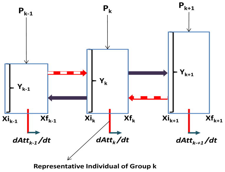
The rate of change of representative individual (dAtt_k/dt) in each sub-population k gives the speed at which the individuals in a sub-population move to the neighboring sub-populations. Positive values for dAtt_k/dt imply that in average individuals in group k are moving to group k+1, whereas negative values imply that individuals in group k are moving to group k−1. In either case, the rate of population leaving group k is a function of dAtt_k/dt, representing how fast the attribute is changing for a representative individual. Besides this speed, the movement between aggregate stocks depends on the vertical length of rectangle associated with group k (i.e., Y_k). This quantity can be calculated using Equation (2), where Y_k is proportional to the frequency of individuals in group k who are subject to crossing sub-population k at the rate dAtt_k/dt.

$$\begin{array}{l}\mathit{Rate}of\mathit{population}\mathit{leaving}\mathit{group}kto\mathit{group}k+1=\mathit{Max}\left(\frac{{\mathit{dAtt}}_k}{d_t}\ast Y_k,0\right)\\ \mathit{Rate}of\mathit{population}\mathit{leaving}\mathit{group}kto\mathit{group}k-1=\mathit{Max}\left(-\frac{{\mathit{dAtt}}_k}{d_t}\ast Y_k,0\right)\end{array}$$ (2)

Similarly, quantify the rates of flow to sub-population k from sub-populations k−1 and/or k+1. The resulting rate of change in population of group k is defined as shown in Equation (3). For k=1 and k=M, there is no neighboring group on the left/right of these groups. Therefore, treat their inflow and outflow components from/to those groups as zero. Figure 3 shows a schematic representation of transition of population between adjacent groups k−1, k, and k+1.

Figure 3.

Schematic representation of transition of population individuals among adjacent groups

$$\begin{array}{l}\mathit{Rate}of\mathit{change}in\mathit{population}of\mathit{group}k=\mathit{Inflow}-\mathit{Outflow}=\\ \left[\mathit{Max}\left(\frac{{\mathit{dAtt}}_{k-1}}{d_t}\ast Y_{k-1},0\right)+\mathit{Max}\left(-\frac{{\mathit{dAtt}}_{k+1}}{d_t}\ast Y_{k+1},0\right)\right]-\mid \frac{{\mathit{dAtt}}_k}{d_t}\mid \ast Y_k\end{array}$$ (3)

Note that the rate of change of the representative individual in group k (dAtt_k/dt) is only used for calculating how many individuals move from group k to group k+1 or k−1 and that it should not actually lead to a change in the position (state) of representative individual k along attribute d. Rather, the representative individual of group k always remains representative for that group, and its state on attribute d does not change. Individuals leaving or joining group k (from other groups) only change the percentage of population in group k. Therefore, dAtt_k/dt should not contribute to any individual-level dynamics in the representative individuals.

Task 3: Estimate the new distribution of population elements along attribute d

Using the rate of change in population in each group calculated in task 2, calculate the stock of population in each group (i.e., P_k) in order to update the estimate for the distribution of population along attribute d by using Equation (1) (i.e., calculating Y_k).

Experimental Setup: Modeling Body Mass Index (BMI) Distribution Dynamics

As a demonstration, we apply our method to capture the distribution of human BMI and how population individuals move from one weight group to another based on the imbalance associated with their energy intake and expenditure. We use an empirical distribution associated with 3074 American women aged 18–74 obtained from the 1999–2003 National Health and Nutrition Examination Survey (NHANES) data to set the initial condition of the simulation. We detail the four steps below.

Step 1

We disaggregate the population into 17 distinct sub-populations corresponding to the following BMI ranges: [14, 16), [16, 18), [18, 20), [20,22), [22,25), [25,28), [28,30), [30,32), [32,34), [34,36), [36,38), [38,40), [40,42), [42,44), [44,46), [46,50), [50,58), where [a, b) represents a≤BMI<b.

Step 2

From the data on the 3074 women, we know the frequency of population in all 17 distinct BMI intervals and use it to initialize the stocks. Using the population in group k (i.e., P_k) and the range of BMI intervals associated with that group, as defined in Step 1, we also estimate the shape of distribution of BMI at the start of the simulation (i.e., calculating Y_k associated with all groups).

Step 3

We construct a micro-level model of the dynamics of weight gain and loss in representative individuals based on the individual-level weight dynamics model for adults developed by Hall, Guo et al. (2009) to capture the energy balance and weight change of individuals over time. Body weight (BW) in their model is represented by two stocks capturing Fat Mass (FM) and Fat Free Mass (FFM) associated with an individual; and the change in body weight is modeled as the result of an imbalance between energy intake (EI) and energy expenditure (EE). Energy expenditure comprises: 1) the Resting Metabolic Rate (RMR), which is the energy required to perform vital body functions while the body is at rest. RMR mainly depends on FM and FFM; 2) the energy needed for physical activity; 3) the energy required for digesting food and nutrients consumed (thermic effect of food); 4) the energy required for developing new mass or digesting existing mass; and 5) the changes in EE due to imbalance between energy intake and expenditure. Equation (4) shows the formula associated with energy expenditure in adults adopted from Hall, Guo et al. (2009):

$$EE=K+{\gamma }_L\mathit{FFM}+{\gamma }_{F}FM+\delta BW+\beta \mathrm{\Delta }EI+{\eta }_F\frac{\mathit{dFM}}{dt}+{\eta }_L\frac{d\mathit{FFM}}{dt}$$ (4)

where γ_L = 22 kcal/(kg.day), γ_F = 3.2 kcal/(kg.day), δ 7 kcal/(kg.day) corresponding to an average sedentary adult, β = 0.24, η_F = 180 kcal/kg, and η_L = 230 kcal/kg. K is a constant determined by the initial energy balance condition. We use a value of 370.21 kcal/day based on the numerical example provided by Chow and Hall. (2008).

Changes in FM and FFM depend on the difference or imbalance between energy intake and energy expenditure (EI-EE). We partition the energy imbalance to be added (if positive) or deducted (if negative) from the FM and FFM stocks. The partitioning function φ for adults is defined as below (Hall, Guo et al. 2009):

$$\phi =\frac{C}{C+FM},C=10.4kg\ast \frac{{\rho }_L}{{\rho }_F}$$ (5)

where ρ_F = 9400 kcal/kg and ρ_F = 1800 kcal/kg. Thus, we obtain the time course of weight loss and gain by solving the following differential equations related to change in FM and FFM (Hall, Guo et al. 2009):

$$\begin{array}{l}\frac{\mathit{dFM}}{dt}=(1-\phi )(EI-EE)/{\rho }_F\\ \frac{d\mathit{FFM}}{dt}=\phi (EI-EE)/{\rho }_L\end{array}$$ (6)

To set the initial values for FM and FFM of representative individuals, we calculate the BMI of the representative individual in each group as the average of the initial and final values of BMI range for the group. Next, we multiply the BMI of the representative individuals by the square of height of the representative individuals to obtain the weights for each group. The height of each representative individual is the average of height of individuals in that group obtained from the empirical dataset and is assumed constant throughout the simulation since this is an adult population. Finally, we obtain the FM and FFM of the representative individuals as the product of their body weights and fat mass fractions. We estimate the fat mass fraction of each representative individual as the empirical average of the fat mass fraction of all individuals in each group.

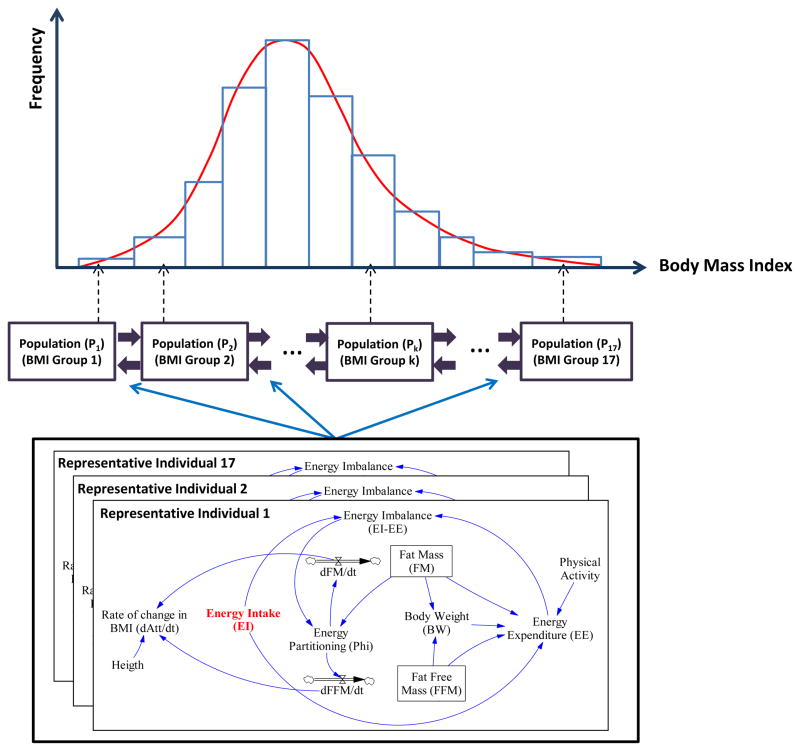
Figure 4 summarizes the system dynamics model structure. The top part of Figure 4 shows the population stock-flow structure, broken out by seventeen categories of BMI. The bottom part of Figure 4 shows the equations regulating body weight of the representative individuals associated with each BMI category.

Figure 4.

Structure of the system dynamics model associated with modeling distribution of BMI

Simulation analysis

We start the simulation from equilibrium in terms of body weight, where the energy intakes of representative individuals equal their energy expenditures. Thus, no change in the population BMI distribution is expected initially. Next, we impose a change in the energy intake of the population at a specific time and estimate the change in the BMI distribution of the population over time.

To validate our method, we compare our results with those from an individual-based model that simulates the change in BMI of 3074 explicitly modeled individual adult women whose initial condition in terms of body weight and body mass fraction has been obtained from the empirical dataset. Thus, the population in the individual-based model has the same initial distribution of BMI as represented in our aggregate model. The individual-based model is structurally similar to that used for the representative individuals (Step 3), but replicated for every member of the population. The only difference is that individual-level model allows FM and FFM for each individual to change due to energy imbalance, where as we keep those constant for the representative individuals so that they do not move along dimension d. We run the individual-based model under a similar scenario, i.e., we start the model from equilibrium where the energy intake of each individual is equal to her energy expenditure. Then we impose the same shock to energy intake of the individuals. See Appendix A for technical details about the formulation used in implementing the shock to energy intake, and the Online Appendix for the simulation models used, documented based on standard model reporting criteria (Rahmandad and Sterman 2012).

Results and Discussion

We run the developed aggregate and individual-based models under two scenarios with respect to change in energy intake of the population. All simulations are conducted in Vensim.

Scenario 1

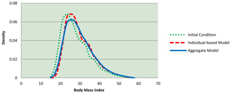
We start the simulation from equilibrium. Starting at year 2, every individual is always given 10 kcal/day more energy intake than what she needs. Implementing the energy intake values for this scenario is straightforward and entails adding the excess energy to the energy expenditure (for items other than weight change) of the representative individual. Figure 5 shows both the initial distribution and the shift in distribution of BMI at year 15 for the models. Note that in scenario 1 the population continues to grow in weight indefinitely, because energy intake is set to be always larger than the current expenditure. Starting from the same initial BMI distribution (the dotted line in Figure 5), we observe that the new distribution of population along attribute BMI obtained using both our method and individual-based model are very similar after 15 simulation year. In fact, the two-sample Kolmogorov-Smirnov test (K-S test) (Sheskin 2003, 453–463) shows that the difference between these two distributions at year 15 is statistically insignificant at the 99% level.

Figure 5.

Shift in distribution of BMI in population after 15 years under scenario 1 which imposes a 10 kcal/day extra energy intake above required for expenditure

We obtain the percentages of the population that are underweight (BMI<20), normal weight (20<=BMI<25), overweight (25<=BMI<30), and obese (BMI>=30) by adding up the percentage of the population in the corresponding BMI groups. Table 1 shows the percentage of population in the four BMI categories estimated by both models in scenario 1. Starting with a 32% prevalence of obesity at the start of simulation, our aggregate model estimates that the prevalence of obesity will reach approximately 41% after 15 years if each individual always takes 10 kcal/day more energy intake than needed. This is close to 40% estimate obtained by the individual-based model.

Table 1.

Comparing weight status distribution obtained from aggregate model and individual-based model

BMI Categories	Initial Condition	Individual-based Model (Year 15)	Aggregate model (Year 15)
Underweight Population (BMI < 20)	0.0905	0.0238	0.0406
Normal Weight Population (20 <=BMI < 25)	0.3270	0.2655	0.2526
Overweight Population (25 <= BMI <30)	0.2602	0.3130	0.2953
Obese population (BMI >= 30)	0.3224	0.3979	0.4115

Scenario 2

We start the simulation from equilibrium, but this time we impose a 200 kcal/day shock to the equilibrium energy intake of every individual in the population after year 2. Due to this shock, individuals with different energy intake levels move across population groups, and because it changes the average energy intake for each representative individual, we cannot calculate it based only on the characteristics of the representative individual. Therefore, in the aggregate model, the consistent calculation of energy intake for each population group requires accounting for energy intake in a co-flow structure (see Appendix A for details). Such auxiliary formulations will be needed in other applications when exogenous inputs influencing the representative element for each sub-population depend on the dynamics of the distribution of interest.

Running both models under the same condition shows that the difference between the two distributions is not statistically significant at the 99% level until about year 6. Figure 6 shows the distribution of population along attribute BMI at the start of simulation (the dotted line) and at year 15 obtained from the aggregate model (the solid line) and the individual-based model (the dashed line).

Figure 6.

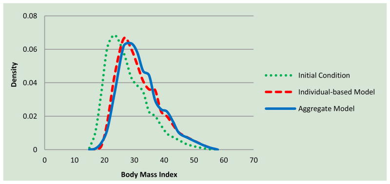
Shift in distribution of BMI in population after 15 simulated years under scenario 2, imposing on each individual 200 kcal/day additional energy intake beyond equilibrium values

Starting from year 7, however, there is a marginally significant difference between the two distributions at the 99% confidence level. In fact, in about year 20 where the population reaches equilibrium, the values for the K-S test statistics and the corresponding 99% critical value are 0.049 and 0.042, respectively. We attribute this difference to the confluence of approximation errors from the co-flows we use to approximate the energy supply for each population group (See Appendix A) and the approximation we use in our core method to estimate population distribution using sub-populations. Nevertheless, the results (Figure 6 and Table 2) show a good correspondence for most practical purposes.

Table 2.

Comparing weight status distribution obtained from our aggregate model and individual-based model under scenario 2

BMI Categories	Initial Condition	Individual-based Model (Year 15)	Aggregate model (Year 15)
Underweight Population (BMI < 20)	0.0905	0.0045	0.0095
Normal Weight Population (20 <=BMI < 25)	0.327	0.1674	0.1271
Overweight Population (25 <= BMI <30)	0.2602	0.3195	0.3128
Obese population (BMI >= 30)	0.3224	0.5086	0.5507

Table 2 shows the percentage of the population in the four BMI categories estimated by both models at year 15 after imposing 200 kcal/day shock to the equilibrium energy intake. Starting with a 32% prevalence of obesity at the start of simulation, the aggregate model estimates that prevalence of obesity will reach 55% after year 6 if we impose a 200 kcal/day shock to energy intake of the population over time. This is close, though not identical, to the 51% estimate obtained by the individual-based model.

Sensitivity Analysis

We expect a better estimate of the distribution of the attribute of interest and its changes over time when we choose narrower ranges for the attribute intervals (bin widths) associated with each sub-population. A similar finding is documented in formulating aging chains (Eberlein and Thompson 2013). To evaluate sensitivity of the aggregate model with respect to the length of bin size, we repeat scenario 1 for sizes 1, 2, 3, 5, and 7 BMI units. We compare the results using the two-sample K-S test. Figure 7 shows the critical value (solid line) at the 99% level and the K-S test statistics corresponding to five different bin sizes. In almost all points of time during the simulation, as the bin size decreases, the value of the K-S test statistic decreases, meaning that our aggregate model develops a more precise estimate of the BMI distribution of the population under analysis if we choose a smaller bin size to estimate the BMI distribution. Moreover, in all cases the differences between the two methods expand over time as the errors due to our approximation accumulate. The K-S test statistic of bin size 7 (the dotted line), which exceeds the critical value around year 10 in the simulation, implies that the difference between the two BMI distributions obtained from aggregate and individual-based models become statistically significant. The smaller bin sizes show no statistically significant difference over 20 years of simulation, and the errors for bin sizes 1 and 2 tend to grow at a much slower rate.

Figure 7.

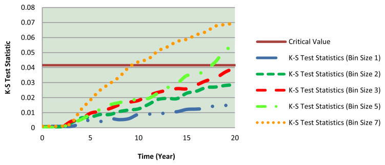
Comparing two-sample K-S test statistics with 99% significance level for bin sizes 1, 2, 3, 5, and 7 BMI units

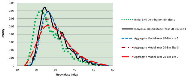
Figure 8 shows the distribution of BMI in year 20 generated by the aggregate model for bin sizes 1, 3, and 7 (the dashed lines with different patterns). Consistent with the K-S test results, the BMI distribution generated with bin size 1 is the closest to the BMI distribution generated by the individual-based model (the solid line), and the difference with bin size 7 is quite visible.

Figure 8.

BMI distribution at year 20 generated by the aggregate model under scenario 1 for bin sizes 1, 3, and 7

In summary, these experiments offer several insights. First, our method is an approximation and the distributions resulting are not identical to the individual-based model. We suggest two reasons for the difference: 1) For nonlinear transformations the representative individual for each group is not a perfect substitute for multiple individuals at different points of the distribution within the corresponding bin, so the behavior of these multiple individuals may not be perfectly estimated by a single representative individual; 2) We approximate the distribution using rectangular bars, and the approximation becomes increasingly coarse with larger bin sizes. We observe an additional difference between the aggregate and individual-based models when a separate approximation, e.g., using co-flows to estimate exogenous inputs, is needed to operationalize the aggregate model (see scenario 2). Second, as a result, the error in approximation is largely due to the size of the bins we use for dividing the sub-population groups. Therefore the approximation becomes very good for small bin sizes; in fact, we conjecture that as we reduce the bin size towards zero, our method converges to simulating the true distribution in deterministic models of large populations. Third, the simulation costs of our method increase linearly with the number of bins.

Similar to setting the time step for a simulation, we recommend performing a sensitivity analysis on the bin sizes to find a value that gives good precision with acceptable computational costs. While smaller bin sizes can increase precision, efficiency is an important consideration if the model is to be used for optimization and calibration experiments where a very large number of simulations should be conducted in the final analysis. Since the bin sizes can be reset with the change of a single parameter (e.g., the dimensionality of the subscript in Vensim), such sensitivity analysis is easy to conduct.

Conclusion

We developed a formulation method that can bridge the micro dynamics associated with elements in a population, and the macro behavior of the population with more precision and significantly less computational costs than individual-based models. The proposed method allows modeling the dynamics associated with the distribution of a population with respect to its attributes. Given that many modeling problems require capturing the heterogeneity of population elements with respect to population attributes, there are many potential applications of this method. For example, it can be used for modeling the distribution of health indicators such as BMI, blood pressure, and blood lipids in human populations, modeling the distribution of skill level or expertise in a firm’s employees, and so forth.

We suggest that the proposed method is most relevant in problem domains where the movement of population elements across different percentiles on the distribution of attributes of interest is a function of an element’s location on the distribution. For example, an individual’s current weight influences the rates of weight gain and loss due to the effect of current weight on her energy expenditure, and consequently her new position along BMI attribute. If such dependence does not exist, the rate of change between different population groups can be formulated without regard for the distribution of interest, and as such will be easy to specify without our method, even though our method should provide consistent results as well.

Even when the rate of change between different population groups does not depend on the position of population individuals along attribute d, the proposed method is beneficial. For example, mortality rate depends on the heterogeneity of population elements along the age attribute, where the shift of population among different age groups is not a function of the age of people. However, evaluating the effect of different interventions on mortality rate may require understanding the individual-level dynamics, especially if the health interventions target factors that are hard to capture via disaggregation. Examples might include interventions focused on particular sub-groups in a heterogeneous population, an individual’s medical history (e.g., outcome of past episodes of care or treatment administered), or contextual factors, such as network position or location, in an irregular space.

In comparison with individual-based models, our method has significantly less computational costs and is easy to apply. We applied our method to a study sample of 3074 American women and simulated the change in distribution of their BMI over time under two scenarios related to changes in their energy intake. Our results showed good precision compared with the results obtained from an individual-based model that explicitly modeled 3074 individuals, but with two orders of magnitude smaller costs, since the aggregate model included computations for 17 representative individuals, whereas the individual-based model included 3074 individuals. In fact, we would have had no additional computational costs if the population had comprised 5 billion individuals. While the computational complexity of the individual-based model grows linearly with the number of individuals, our method’s complexity only grows with the number of aggregate population groups and irrespective of the number of individuals. This finding suggests that the proposed method can provide significant efficiencies where calibration and extensive sensitivity analysis need to be run on large datasets.

Our study also has some limitations. First, our empirical example is mainly for demonstrative purposes and does not reflect realistic public health outcomes. Moreover, our method can only be used when disaggregating the population along one attribute. Extrapolation to multiple attributes is conceptually not very different and makes a great extension. Specifically, rather than breaking a one-dimensional distribution into intervals, a multi-dimensional distribution could be approximated by multi-dimensional (hyper) rectangles, although such extensions could be computationally expensive. For example, with two attributes and M and N groups in each, there will be M*N population groups for which we have to specify the aggregate transition rates, and the complexity will grow exponentially with the number of attributes. Another extension of our method would be to incorporate stochastic movements across population groups. We currently work with individual-level models that are deterministic and therefore dAtt_k/dt is either positive or negative. However, many random factors may influence the individual-level model, and therefore some individuals may move to group k+1 while some others may move to group k−1 at the same time. Consistently aggregating the stochastic effects of random factors to the aggregate flow rates across population groups offers another exciting research problem.

Overall we hope this method offers an attractive tool for modelers who want to efficiently and accurately portray changes in population distributions over time and we look forward to future extensions that increase the versatility of the method.

Appendix A: Formulating Population Energy Intake

Energy intake (from food consumption) is an exogenous input that controls the rates of body weight change. This input can be specified numerically, or as a fraction of current energy expenditure, in an easy and consistent way across both aggregate and individual-based models. Implementing scenario 1 (10 kcal/day more energy intake than expenditure) is easy, i.e. we give the representative individual her energy expenditure plus 10 kcal/day. However, specifying this input consistently across the two models requires care when the individual-based model uses exogenous shocks, i.e., scenario 2, which adds a constant 200 kcal/day extra energy intake to the initial intake. Therefore, in scenario 2 we use co-flows to capture the stock of total energy supply (intake) associated with each population group in our aggregate model. These co-flows enable us to consistently keep track of the energy supply for each population group and the individuals within it in parallel to what occurs in the individual-based model. Below, we provide the details of this formulation to facilitate such applications in diverse modeling problems.

When population is in equilibrium in terms of weight, the energy supply (energy intake) is equal to the energy demand (energy expenditure) for the whole population and similarly, for each representative individual. Thus, we calculate the initial value associated with energy intake stock of each population group by multiplying the energy demand of the representative individual in each group by the number of individuals in that group. Whenever we change the energy intake of a population group, the change is accumulated in the energy stock associated with that group. Thus, at any point in time we have total energy supply associated with each group in the co-flows. By dividing the total energy stock of each group by the number of people in that group, we obtain the average energy supply for representative individual for each group. Using the energy supply of each representative individual as the energy intake of representative individual to calculate the rate of change in the BMI of that representative individual allows us to determine the rate of change in the respective population group.

As individuals leave or are added to population group stocks, we also need to capture how much energy is removed or added to the co-flow energy stocks corresponding to the population groups. To do so, we mimic what happens in an individual-level model: an individual leaving one BMI group also removes her energy intake, which is reflected in the total energy of that group. The following steps to be taken at every time step calculate the energy removed from a population group (say, group k) and added to the neighbor group k+1, when an individual moves from group k to group k+1 (the same logic applies to all groups):

1. Calculate the energy required (energy demand) of an individual standing in the border of groups k and k+1. We call this individual a “marginal individual” associated with groups k and k+1. Calculate the energy demand associated with the marginal individual as the weighted average of energy demand (energy expenditure) of the representative individuals associated with groups k and k+1. Note that these weights are based on the distance of the marginal individual from the representative individuals in each group, such that the representative individual who is closer to the marginal individual receives a higher weight.

   As an example, assume two adjacent groups corresponding to BMI ranges [20, 22) and [22, 26), respectively. Also assume that the energy expenditures of the representative individuals associated with each group are 1600 kcal/day and 1750 kcal/day, respectively. For an individual standing at the margin of BMI 22, her distance to the representative individual of the [20, 22) group is 1, whereas her distance to the representative individual of the [22, 26) group is 2. Thus, the energy expenditure (energy demand) associated with this marginal individual is calculated as $\frac{2}{3}\ast 1600+\frac{1}{3}\ast 1750=1650\mathit{kcal}$.

2. Calculate the ratio of energy supply (energy intake) to energy demand (energy expenditure) for the representative individual of group k. Obtain the energy supply of each representative individual by dividing the energy supply stock of that group by the population stock of the group. Thus, the energy demand associated with each representative individual is equal to the energy expenditure calculated by the micro-level model.

3. Multiply the energy demand of the marginal individual between groups k and k+1 by the ratio of energy supply to demand calculated for representative individual in group k. The obtained result is the energy (intake) that the marginal individual between group k and k+1 takes to group k+1 as she moves from group k to group k+1. Multiply this energy by the flow of individuals moving from group k to group k+1 to find the total energy intake removed from group k to group k+1.

Similar steps calculate the energy taken from population group k+1 and added to neighbor group k, when individuals move from group k+1 to group k (i.e., losing weight):

1. Calculate the energy required (energy demand) of the “marginal individual” associated with groups k and k+1.

2. Calculate the ratio of energy supply to energy demand for the representative individual of group k+1.

3. Multiply the energy demand of the marginal individual between groups k and k+1 by the ratio of energy supply to demand calculated for the representative individual of group k+1. The obtained result is the energy intake that the marginal individual between group k and k+1 takes to group k as she moves from group k+1 to group k. Multiply this energy by the number of people moving from group k+1 to group k to calculate the total energy intake removed from group k+1 to group k.

The fully formulated models for this scenario are included in the Online Appendix.

References

- Chow CC, Hall KD. The dynamics of human body weight change. PLoS Computational Biology. 2008;4(3):1000045. doi: 10.1371/journal.pcbi.1000045. [DOI] [PMC free article] [PubMed] [Google Scholar]
- Eberlein RL, Thompson JP. Precise modeling of aging populations. System Dynamics Review. 2013;29(2):87–101. [Google Scholar]
- Größler A, Zock A. Supporting Long-term Workforce Planning with a Dynamic Aging Chain Model: A Case Study from the Service Industry. Human Resource Management. 2010;49(5):829–848. [Google Scholar]
- Hall KD, Guo J, et al. The Progressive Increase of Food Waste in America and Its Environmental Impact. PLoS ONE. 2009;4(11):e7940. doi: 10.1371/journal.pone.0007940. doi:7910.1371/journal.pone.0007940. [DOI] [PMC free article] [PubMed] [Google Scholar]
- Homer J, Milstein B, et al. Obesity population dynamics: Exploring historical growth and plausible futures in the U.S. Proceedings of the 24th International System Dynamics Conference; Nijmegen. 2006. [Google Scholar]
- NHANES. Centers for Disease Control and Prevention (CDC/NHANES) National Health and Nutrition Examination Survey. 2013. [Google Scholar]
- Osgood N. Representing heterogeneity in complex feedback system modeling: Computational resource and error scaling. Proceedings of the 22nd International Conference of the System Dynamics Society; Oxford. 2004. [Google Scholar]
- Osgood N. Lightening the performance burden of individual-based models through dimensional analysis and scale modeling. System Dynamics Review. 2009;25:101–134. [Google Scholar]
- Rahmandad H, Sabounchi NSZ. Building and estimating a dynamic model of weight gain and loss for individuals and populations. The 29th International Conference of the System Dynamics Society; Washington, DC. 2011. [Google Scholar]
- Rahmandad H, Sterman JD. Heterogeneity and network structure in the dynamics of diffusion: Comparing agent-based and differential equation models. Management Science. 2008;54(5):998–1014. [Google Scholar]
- Rahmandad H, Sterman JD. Reporting guidelines for simulation-based research in social sciences. System Dynamics Review. 2012;28(4):396–411. [Google Scholar]
- Schwarz R, Maybaun P. Dynamics of depreciation and scrapping in Business Economics. Proceedings of the 22nd International Conference of the System Dynamics Society; Oxford. 2004. [Google Scholar]
- Sheskin DJ. Handbook of Parametric and Nonparametric Statistical Procedures. 3. Florida, USA: Chapman and Hall/CRC; 2003. [Google Scholar]
- Snabe B. Dissertation. Germany: Universität Mannheim; 2006. The Usage of System Dynamics in Organizational Interventions. [Google Scholar]
- Sterman JD. Business Dynamics: Systems Thinking and Modeling for a Complex World. New York: McGraw-Hill; 2000. [Google Scholar]