. 2015 Jan 23;4:e04919. doi: 10.7554/eLife.04919

Figure 3. Multivariate analysis reveals two temporal components of evoked response to visual stimuli.

(A) Multivariate decoding performed well to predict the category of photograph (Si) in the Association phase. Cross-validated linear SVM prediction accuracy using all 275 sensors at each time bin is shown. A pattern of two distinct peaks in classifier accuracy around 200 ms and 400 ms after Si onset is evident. (B) At 200 ms after Si onset, there was no difference in representational similarity between same-category and different-category Si objects (left panel, p = 0.2 by t-test between subjects). At 400 ms, representational similarity was higher for same-category than different-category objects (right panel, p = 5 × 10⁻⁷). F1–F4, B1–B4 and S1–S4 refer to the unique faces, bodies and scenes presented during the Association phase. (C) When discriminating fractal identity (i.e., a 6-way classification problem of stimuli with no natural categories), performance was sharply peaked before 200 ms after fractal onset. Shaded area shows standard error of the mean.

DOI: http://dx.doi.org/10.7554/eLife.04919.005

Figure 3.

Figure 3—figure supplement 1. Univariate classification using best sensor.

Figure 3—figure supplement 1.

We tested the capacity of the most discriminative single sensor (selected separately for each subject) to predict the Si category, using linear support vector machines (SVM) with a single feature. The accuracy of this univariate classifier peaked at 47.4 ± 1.3% in cross-validation (red trace). (When using a nearest-mean univariate classifier rather than a univariate SVM, accuracy peaked at 45.6 ± 1.9%.) We constructed independent null distributions at each time bin by repeating this procedure 100 times with randomly shuffled category labels. At 200 ms post-stimulus, the median of the null distribution was 37.0% accuracy (greater than 1/3rd due to allowing the best sensor for each subject), while the 95th percentile of the null distribution was 38.6%. Blue line shown is multivariate SVM performance, from Figure 3A, for comparison.
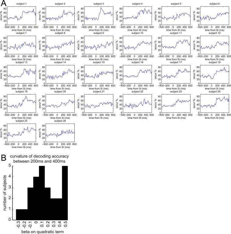
Figure 3—figure supplement 2. Multivariate classification of Si for individual subjects.

Figure 3—figure supplement 2.

(A) Classification accuracy in predicting Si category in Association phase for individual subjects. (B) We fit regression models to each subject's accuracy curve (between 200 ms and 400 ms), with constant, linear, and quadratic terms. This histogram shows the estimated betas on the quadratic term. Positive beta indicates positive curvature of the accuracy curve between 200 ms and 400 ms. No individual subject reached Bonferroni-corrected significant betas on the quadratic term of the regression.
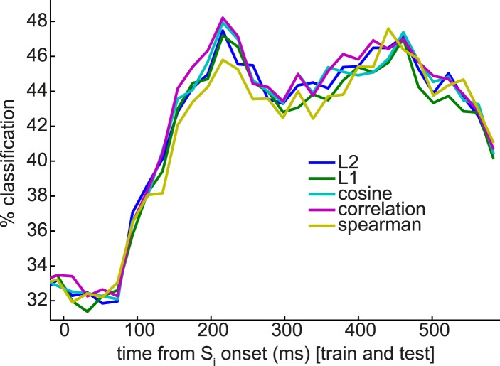
Figure 3—figure supplement 3. Nearest-mean multivariate classifiers, under a variety of distance metrics, underperform SVM but extract a similar pattern of multiple peaks in classification performance.

Figure 3—figure supplement 3.

Compare to SVM applied to the same classification problem in Figure 3B, blue trace.
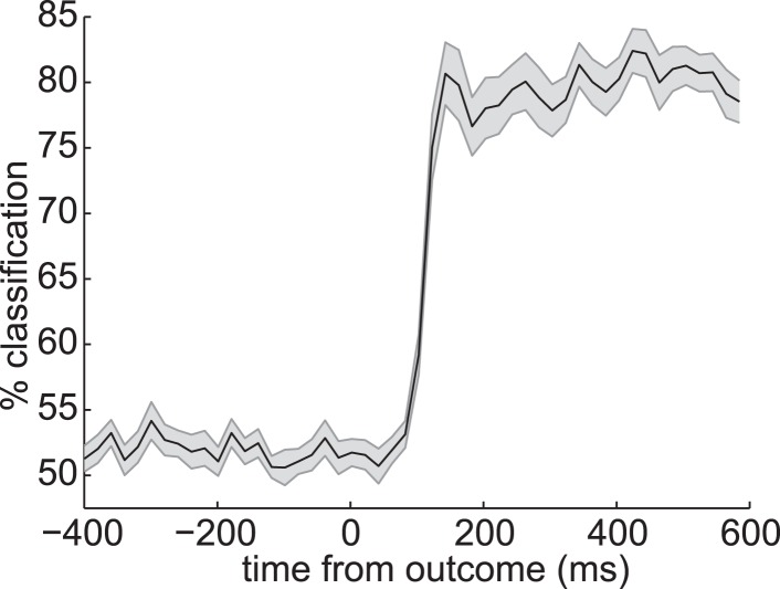
Figure 3—figure supplement 4. Decoding outcome identity.

Figure 3—figure supplement 4.

At the time of outcome, there was a strong neural representation of the identity of the outcome itself (the coin or blue square). Together with Figure 3D, this suggests that the neural signal at time of Sd and outcome strongly encoded a representation of the on-screen stimulus.
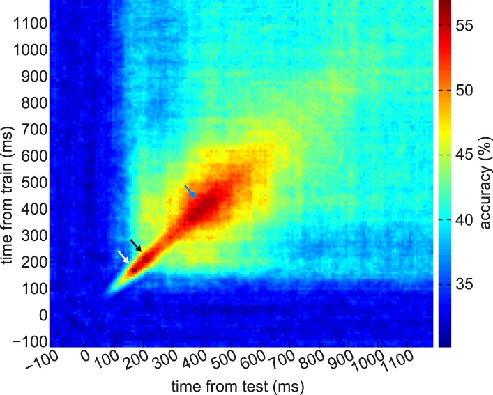
Figure 3—figure supplement 5. Generalization of instantaneous representational patterns over time, with finer temporal binning.

Figure 3—figure supplement 5.

Here we trained classifiers on every time bin relative to the onset of Si in the Association phase, and tested at every time bin relative to the same onsets. For this figure we binned the data into 8 ms bins rather than the 20 ms bins used in the rest of the paper. Each cell of this grid shows cross-validated prediction accuracy, so the diagonal is equivalent to Figure 3B, blue trace (except that this figure has finer temporal binning). Later classifiers generalized better over time than earlier classifiers. We note the possibility that the 200 ms peak of classification might be decomposed into further sub-peaks (white and black arrows); however, we were unable to statistically separate these sub-peaks, due to variability between subjects. The peak at 400 ms is evident (blue arrow). Absolute classification accuracy is lower than with more coarsely binned data, likely due to a poorer signal to noise ratio.
Figure 3—figure supplement 6. Image statistics.

Figure 3—figure supplement 6.

Image types varied in low-level visual properties as well as shape. The methods we used are agnostic as to the kinds of features that drove the neural representation of category.