Uncontrolled combustion of shredded tires in a landfill -Part 2: Population exposure, public health response, and an air quality index for urban fires

Abstract

The Iowa City Landfill in eastern Iowa, United States, experienced a fire lasting 18 days in 2012, in which a drainage layer of over 1 million shredded tires burned, generating smoke that impacted the surrounding metropolitan area of 130,000 people. This emergency required air monitoring, risk assessment, dispersion modeling, and public notification. This paper quantifies the impact of the fire on local air quality and proposes a monitoring approach and an Air Quality Index (AQI) for use in future tire fires and other urban fires. Individual fire pollutants are ranked for acute and cancer relative risks using hazard ratios, with the highest acute hazard ratios attributed to SO₂, particulate matter, and aldehydes. Using a dispersion model in conjunction with the new AQI, we estimate that smoke concentrations reached unhealthy outdoor levels for sensitive groups out to distances of 3.1 km and 18 km at 24-h and 1-h average times, respectively. Modeled and measured concentrations of PM_2.5 from smoke and other compounds such as VOCs and benzo[a]pyrene are presented at a range of distances and averaging times, and the corresponding cancer risks are discussed. Through reflection on the air quality response to the event, consideration of cancer and acute risks, and comparison to other tire fires, we recommend that all landfills with shredded tire liners plan for hazmat fire emergencies. A companion paper presents emission factors and detailed smoke characterization.

1. Introduction

Shredded tire chips are commonly used as landfill drainage lining material. They are permeable to leachate and protect the landfill liner (Cecich et al., 1996; FEMA/USFA, 2002; Fiksel et al., 2011; IWMB, 2002; Warith and Rao, 2006). This practice also offers a way to dispose of scrap tires (FEMA/USFA, 2002). However, shredded and whole tires pose a significant fire risk; they are difficult to extinguish once ignited and emit criteria pollutants and air toxics when combusted (Lemieux et al., 2004; Lemieux and Ryan, 1993; USFA, 1998; Wang et al., 2007).

The Iowa City landfill's shredded tire drainage layer was accidentally ignited and burned openly for 18 days beginning May 26, 2012 (Figure 1). The exposed shredded tire drainage layer was 1-m thick and covered 30,000 m² and the fire consumed an estimated 1.3 million tires (20,540 metric tons, assuming 15.8 kg tire^-1; RMA 2013). The Iowa City landfill was close enough to population centers of Johnson County, Iowa (population 152,586, U.S. 2010 Census) to impact people through smoke exposure, including densely populated neighborhoods.

Figure 1.

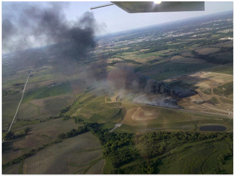
Photograph of the Iowa City landfill fire, with smoke primarily from the burning shredded tire drainage layer

Over a dozen major tire fires have occurred in the United States and Canada since 1983 (see CalEPA, 2002; DEQ, 1989, USFA, 1998; EPA 1997; Ritter, 2013). The Iowa City landfill fire was approximately five times smaller than the largest U.S. tire fire, the 1983 Rhinehart fire (Ritter, 2013). These types of fires often exceed one month in duration and pose threats to the health and safety of both firefighters and the public. In some cases, fires have prompted voluntary evacuations, school closings, and increased respiratory complaints. On occasion, tire fires have been documented through published air concentration measurements from environmental agencies (CalEPA, 2002; EPA, 1997; OMOE, 1990; Sidhu et al., 2006; USFA, 1998). Sampling results for polycyclic aromatic hydrocarbons (PAH) and metal residues on vegetation are also reported (CalEPA, 2002; Steer et al., 1995), as well as cancer risk assessment conducted using B[a]P concentrations (Sidhu, et al., 2006). While the Iowa City fire shares many similarities to the listed tire fires, it is, to our knowledge, the first major U.S. tire fire occurring in a landfill liner system instead of at a tire stockpile location.

From public health and air quality perspectives, the response to a large scale tire fire includes many decisions – what compounds to monitor; where to locate air monitors; whether to use mobile or fixed samplers; whether to use integrating or continuous techniques; interpretation of multi-pollutant mixture results across varied averaging times; action levels for warnings, evacuations, and closures; wording of public notices; recommended actions for reducing exposure; and best practices for using dispersion modeling.

Existing reports from past fires have major shortcomings as a guide to the public health response (JCPHD, 2012, Downard et al., co-submitted). Shortcomings include a lack of prioritization on what to measure and where to measure it, and a focus on reporting concentrations with limited interpretation of the public health impact. Past ambient studies rarely incorporate correction for dilution levels – limiting ability to generalize from measurements. Finally, variety in analyte selection and monitoring protocol is a challenge, with the monitoring focus varying among PAH, volatile organic compounds (VOCs), fine particulate matter (PM_2.5), and CO (CalEPA, 2002).

During the Iowa City incident, the public health response was led by the Johnson County Department of Public Health (JCPH) supported by State Hygienic Lab (SHL), the Iowa Department of Natural Resources (IDNR), EPA Region 7, and the University of Iowa. The combined measurement of various pollutants (see Downard et al., co submitted) and modeling work by these organizations enabled retrospective characterization of ambient concentrations.

This paper attempts to improve on the air quality response through a hierarchy of monitoring priorities for large scale tire fires, a tire fire irritant Air Quality Index (AQI) for interpretation of the measured values, and a ranking of tire fire components by acute and cancer hazard ratios. We also examine public health response guidelines and estimate emissions of some compounds not yet sampled in tire burning by using emissions profiles from open burning of oil (Booher, 1997; Lemieux, 2004). This work focuses on ambient air pollutants, and does not deal with the many other aspects of the emergency response.

2. Methods

2.1 Monitoring Sites and Instrumentation

Ambient air, often impacted with smoke, was examined at a variety of sites as mapped in Figure 2. Detailed descriptions of methods and instrumentation used to measure CO_2, CO, SO₂, particle number, PM_2.5, PM₁₀, PAH, and trace metals are in Downard et al. (co-submitted). Only additional measurements and site descriptions, as related to dispersion modeling and public health response, are described here. Additional information on detailed site locations, instruments deployed, and laboratory methodologies are located in Supplementary materials.

Figure 2.

Map of the study area shaded by Census 2010 block group population density (persons/km²). Symbols mark locations of air quality samples from mobile sampling (green triangles), VOC grab samples (yellow circles), and long-term PM_2.5 monitors (red circles). Concentric circles mark radii of 1.6 km (1 mi, red), 3.2 km (2 mi, yellow), and 6.4 km (4 mi, blue) from the fire location.

Ambient VOC concentrations were determined by EPA methods TO-12 and TO-15 (EPA, 1999). Ten grab samples, representing background and plume-impacted air, were collected in pre-cleaned 6-L Summa canisters (Entech Silonite™). Analysis was by gas chromatography (GC) mass spectrometry (Agilent Technologies 7890A, 5975C; 60 m DB-1 column).

Two stationary sites were critical to monitoring. Hoover Elementary School (EPA 191032001) is located 10.5 km east of the Iowa City landfill in a residential area. This station monitors for 24-h average and hourly PM_2.5 using a low volume FRM sequential air sampler (R&P Model 2025 w/VSCC gravimetric) and a beta attenuation sampler (Met One BAM-1020 w/SCC beta attenuation), respectively. The University of Iowa Air Monitoring Site (IA-AMS) is located 4.2 km northeast of the landfill and is situated among recreational fields, low use parking areas, and woodlands.

2.2 Hazard ratios for tire fire smoke

Hazard ratios compare the ambient concentrations of pollutants to reference concentrations for a similar averaging period (EPA, 1989). The hazard ratio concept can be used to target specific pollutants in an exposure situation (Austin, 2008; EPA, 1989; McKenzie et al., 2012; Silverman et al., 2007). The hazard ratio (HR_i) for species i is

$${\mathit{\text{HR}}}_i=\frac{c_i}{c_{\mathit{\text{ref}}}}$$ (1)

where c_i is the ambient concentration and c_ref is the reference concentration. For the acute hazard ratio (HRA) we adopt 1-h Acute Exposure Guideline Levels (AEGL-1) (NRC, 2001) for c_ref. AEGL-1 is defined as “the airborne concentration of a substance above which it is predicted that the general population, including susceptible individuals, could experience notable discomfort, irritation, or certain asymptomatic nonsensory effects. However, the effects are not disabling and are transient and reversible upon cessation of exposure.” AEGL values were selected because they were developed specifically for emergency exposures and are thoroughly documented. For species with no 1-h AEGL, a Short Term Exposure Limit (STEL) from the American Conference of Industrial Hygienists (ACGIH, 2014), with the NIOSH STEL, OSHA STEL, and five times the TLV-TWA for the compound as alternate c_ref depending on availability (OSHA, 2006, NIOSH, 1996). For the cancer risk hazard (HRC), the inverse of the inhalation unit risk factor (IUR) from IRIS (EPA, 2011) or CalEPA (CalEPA, 2003) was used for c_ref.

Because individual tire fire studies lack comprehensive species coverage, ratios were calculated from multiple studies (EPA, 1997; CalEPA, 2002; Downard et al., co-submitted), ranked within study, and then merged into a unified ranking. Because no tire fire study included some compounds such as formaldehyde, a laboratory study of pooled crude oil burning was also included (Lemieux et al., 2004).

2.3 Development of Air Quality Index (AQI) for tire fires

Air quality indices (AQI) are useful for communication of the level of hazard (Chen et al., 2013; Dimitriou et al., 2013; EPA, 2006; Gurjar et al., 2008; OEHHA, 2012). However, traditional AQI formulas have drawbacks when applied to an emergency fire situation – 1-h, 8-h and 24-h averaging time AQI are needed but are not available for all pollutants, and it is not clear how to account for the multi-pollutant nature of the smoke. Factors such as tire particulate toxicity and the high mutagenicity of tire fire smoke relative to wood smoke (Lemieux and Ryan, 1993; Lindbom et al., 2006) suggest that conventional indices may be insufficient for tire fire smoke. We propose an AQI formula for total air quality index (a_tot) from summation of the impacts from multiple pollutants:

$$a_{\mathit{\text{tot}}}={\left[a_{\mathit{\text{PM}}}^p+o_1^p+o_2^p+\cdots +o_m^p+u_1^p+u_2^p+\cdots +u_n^p\right]}^{1/p}$$ (2)

Equation 2 includes the concentrations of PM_2.5 (a_PM), m co-pollutants (o_m), and n unmeasured compounds (u_n). Summation is appropriate when pollutants share a common health effect and mode of action (Murena, 2004; Plaia and Ruggieri, 2011). In the case of the tire fire smoke, most of the pollutants are respiratory irritants, and we propose summation over the irritant compounds. The exponent (p) controls the nature of the summation process; as p increases, the summation becomes dominated by the highest air quality index in the summation. A fixed p value of 2.5 has been proposed (Kyrkilis et al., 2007), which heavily weights the maximum AQI. In this study, results from p exponents of both 1 and 2.5 are explored, and the main results and discussion are reported using a p exponent of 1.

The AQI values for all compounds were calculated using linear interpolation between AQI breakpoints (EPA, 2009). Breakpoints for PM_2.5 were from OEHHA (2012), which are based on the EPA NAAQS but extend to 8-h and 1-h averaging periods. The NAAQS-based SO₂ AQI breakpoints are adopted uniformly for 24-h, 8-h, and 1-h averaging times.

For all other species, NAAQS based thresholds are not available, and AEGL were used if available. A full complement of AEGL mixing ratios consists of 15 values, corresponding to 5 averaging times and 3 thresholds: AEGL-1 (defined in section 2.2), AEGL-2 (irreversible or other serious adverse health effects), and AEGL-3 (life-threatening). For some compounds, AEGL concentrations are not available, and the AQI breakpoints rely on STEL instead, as described in section 2.2. Due to the high concentrations involved in the tire fire, and the high STEL and AEGL of some compounds, linear extrapolation of AQI values in excess of 500 was performed.

SO₂ has NAAQS-based AQI breakpoints as well as AEGL values and a STEL. Therefore, it is used to translate from concentrations relative to AEGL or STEL (available for many compounds) to concentrations relative to an AQI (available for SO₂). Specifically, the AQI of pollutant i is calculated by

$$a_i=a_{\mathit{\text{SO}}2}\left(f_{\mathit{\text{AEGL}}}^{-1}\right({\overline{\mathit{\text{AEGL}}}}_{\mathit{\text{SO}}2},f_{\mathit{\text{AEGL}}}({\overline{\mathit{\text{AEGL}}}}_{\iota },c_i)\left)\right)$$ (3)

where f_AEGL is a piecewise linear function with two inputs: (a) the 3 AEGL values of species i (denoted by the vector $\overline{{\mathit{\text{AEGL}}}_{\iota }}$), and (b) c_i. f_AEGL is 0 at c_i of 0, and 1, 2 and 3, respectively at concentrations of AEGL-1, AEGL-2, and AEGL-3. $f_{\mathit{\text{AEGL}}}^{-1}$ is the inverse function that returns the concentration that will give a specific value of f_AEGL For SO₂, the AEGL-1, 2, and 3 mixing ratios are 200, 750, and 30,000 ppb, respectively. The 1-h NAAQS (also the value for an AQI of 100) is 75 ppb, and the STEL is 250 ppb. Therefore, for S0₂, the AEGL-1, 2, and 3 values occur at AQI values of 224, 700, and 28,000, respectively, and the SO₂ STEL occurs at an AQI value of 256.

PM_2.5 was used as a tracer of the tire fire smoke. That is, we considered tire fire smoke by its PM_2.5 concentration (denoted PM_t), and then calculate the concentrations of all co-pollutants (e.g. SO₂, formaldehyde, VOCs) using the ratio of the co-pollutant emission factor to that of PM_t. The various AQI values are combined according to equation 2. An example 1-h AQI calculation is shown in Supplementary materials.

2.4 Dispersion modeling

Two dispersion models, Hazard Prediction and Assessment Capability model (HPAC) version 5.0 MB (Sykes and Gabruk, 1997) and AERMOD (EPA-454/R-03-004, September 2004 release 0726) (EPA, 2004) were run independently, with results first available beginning on May 30, the fourth full day of the fire. Both models were provided to the incident command group to help plan activities, and to understand potential impacts on populated areas (Holmes and Morawska, 2006; Kakosimos et al., 2011; Morra et al., 2009).

The Iowa National Guard's 71^st Civil Support Team requested dispersion modeling from the Defense Threat Reduction Agency (DTRA). DTRA modeled the landfill fire as combustion of oil using HPAC.

AERMOD (EPA-454/R-03-004, September 2004 release 0726) (EPA, 2004) was used with regional forecast meteorology (60 hour forecast) from the Weather Research and Forecasting model (WRF) 3.3.1 (Skamarock et al., 2008). The WRF configuration included 24 vertical layers from the surface to 5 km, 4 km horizontal resolution, ACM2 planetary boundary layer scheme (Pleim, 2007), and initial conditions and observational constraint from the North American Mesoscale Model. WRF profiles were processed for AERMOD using MCIP2AERMOD (Davis et al., 2008).

WRF/AERMOD simulated dispersion to a 100 m receptor grid from an area source covering the burning landfill cells. All receptors were placed 2 m above terrain height. In forecasting, the smoke PM_2.5 emission rate was set at 0.4 g/s (10 μg/m²-s) to match early field observations of the plume (site BDR on May 30, 20:00). For retrospective modeling to reconstruct concentrations, the emission rate for smoke was adjusted to minimize the average of the absolute fraction errors of observed plumes. Specifically, the peak model concentration at the distance of the monitoring location was compared to the observed peak at 10 min averaging time (where available) or hourly average concentration. Cases with the modeled plume more than 40° away from the measurement location were excluded.

3. Results and Discussion

The fire was first reported during the evening of May 26, 2012. The impact of the landfill fire plume on individual stationary sites was episodic and depended strongly on wind direction, dilution, and emission rates that vary due to firefighting activities, temperature, and atmospheric conditions (Akagi et al., 2012; CalEPA, 2002; JCPHD, 2012; Kwon and Castaldi, 2009). The tire fire was declared under control and smoke emission was almost eliminated as of June 12, 2012. The plume was well-dispersed during a majority of the fire-affected period due to meteorology. During these periods, its influence was localized. Conversely, two stable periods with low boundary layer heights and significant smoke accumulation over more widespread areas were identified (June 1-3 and June 7-8). Chronology of weather, PM concentrations, sampler activities, and model highlights are found in Supplementary materials. Concentrations of PM_2.5, SO₂, and PAH were used to develop emission factors and are discussed in Downard et al. (co-submitted). VOC concentrations are reported in section 3.1 prior to their use in hazard ratio calculations.

3.1 VOC

A total of 54 VOCs were quantified from May 27 to June 2 in both background and impacted locations. Tire fires are known to be a major source of VOCs (Lemieux and Ryan, 1993). Table 3 reports a selected list of VOC concentrations in a representative plume-impacted sample taken on May 28 at 300 m from the fire with additional data in Supplementary materials. Significant increments in concentration over background were observed for many aromatic VOCs such as benzene, toluene, ethyl toluene, dimethyl benzene, xylene and styrene, as well as aliphatics (e.g., propane, butane). Fewer carbonyls were measured, but acrolein showed enhancement. Several hydrocarbon concentrations were below detection limit.

Table 3.

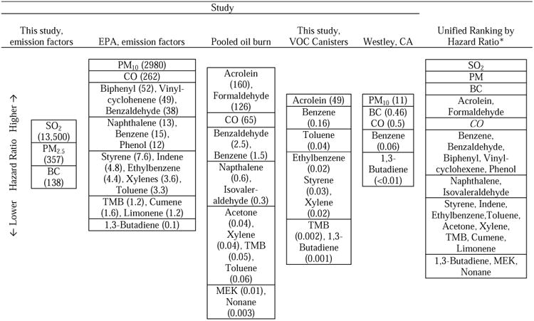
Ranked order of acute hazard ratios from multiple studies and unified ranked order list of hazard ratios. Numbers in parentheses are the hazard ratios (see text).

^*In the unified list (rightmost column), regular typeface indicates respiratory irritation or reduced lung function as part of the acute effect; italic typeface indicates that respiratory irritation or reduced lung function is NOT part of the acute effect. This is the case only for carbon monoxide.

Benzene concentrations ranged from 0.05-0.07 ppbv in background samples and increased to 8.3 ppbv and remained elevated in some samples (e.g., 0.63 ppbv 8.0 km downwind). Toluene was present at 8.7 ppbv in the plume and 0.50 ppbv downwind. Synthetic rubber components butadiene and styrene are typically below detection limits in Iowa City but were 0.5-1 ppbv at 300 m from the fire. The benzene concentrations were well below a number of relevant reference concentrations, such as the OSHA STEL (1000 ppb), the ACGIH TLV-TWA (100 ppb), and the AEGL-1 (52,000 ppb, 1-h) but close to the lower ATSDR minimum risk level of 9 ppb (ATSDR 2013).

3.2 Identification of key pollutants from hazard ratio analysis

Calculated cancer and acute hazard ratios (HRA and HRC) are summarized in Tables 2 and 3, respectively, with details on ambient concentration measurements and reference concentration values, from multiple studies in Supplementary materials. Acute hazard ratios can be found in the parenthesis in Table 2. Note that hazard ratios from different ambient concentration measurements (e.g., the Westley vs. the Iowa City VOCs) cannot be directly compared to each other or to the hazard ratios based on emission factors. Only the relative orderings can be compared. SO₂, PM_2.5, black carbon (BC), and air toxic VOCs had the highest rankings when assessed using concentrations or emission factors from Iowa City. In other studies with tire smoke, BC, biphenyl, benzene, benzaldehyde, PM, and CO were highly ranked hazards. SO₂, which receives the highest ranking by AEGL-based hazard ranking has limited published emission factors. For example, it is not listed as an emission factor in Lemieux and Ryan (1993); however, Lemieux and Ryan did publish an SO₂ and CO time series for a tire fire test that corroborates the high placement of SO₂ in our hazard ratio ranking. The test had an SO₂/CO mixing ratio of ∼0.2-0.33 which corresponds to HRA_SO2/HRA_CO of 400-660.

Table 2.

Cancer hazard ratios derived from concentrations or emission factors from this work and from other ambient and laboratory combustion studies.

CAS Number	Species of Interest	Unit Risk Factor (URF)	EPA Classification	Laboratory open tire fire burn			Westley Tire Fire			This study (VOC canister)			This study (emission factors)			Pooled Oil Burning
		[(μg/m3)-1]		EF (mg kg-1)	HRC	Rank	Cone.(μg m-3)	HRC	Rank	Cone.(μg m-3)	HRC	Rank	EF (mg kg-1)	HRC	Rank	EF (mg kg-1)	HRC	Rank
	PM2.5	3.0×10-4											5350	1.6	1
71-43-2	Benzene	2.9×10-5	A	2205	0.064	2	9.2	2.7×10-4	1	26.4	7.7×10-4	1				251	7.3×10-3	1
91-20-3	Naphthalene (a)	3.4×10-5	C	1195	0.041	3
106-99-0	1,3-Butadiene	1.7×10-4	B2	160	0.027	3	1.1	1.9×10-4	2	1.5	2.6×10-4	2
100-41-4	Ethylbenzene	2.5×10-6	D	632	0.0016	4				2.9	7.2×10-6	3				10	2.5×10-5	4
50-00-0	Formaldehyde	6.0×10-6	B1													139	8.3×10-4	2
75-07-0	Acetaldehyde	2.7×10-6	B2													44	1.2×10-4	3
50-32-8	Benzo(a) pyrene	1.1×10-3	A	113.9	0.13	1	0.15	1.7×10-4	2				3.56	3.9×10-3	2	7	7.7×10-3	1

^(a)Volatile and semi-volatile phase

Aldehydes have not been extensively measured in tire fire emissions, but are known components of smoke from burning oil. Aldehydes include strong irritants with low reference concentrations, and formaldehyde, benzaldehyde, and acrolein have high rankings according to their HRA. Accordingly, we expect these compounds to play a role in the health impacts of the smoke, and recommend further study of their emissions.

Hazard ratio rankings within an order of magnitude of each other were grouped to generate a merged ranked list of the most hazardous compounds found in the righthand column of Table 2. Compounds common to multiple studies (benzene, 1,3-butadiene, PM and CO) provided benchmarks for relative rankings. The unified acute hazard ratio for tire fires includes SO₂ > PM > BC> Acrolein, Formaldehyde > CO > Benzene, Benzaldehyde, Biphenyl, 4-Vinyl-l-Cyclohexene, and Phenol as the higher ranked compounds. Monitoring and risk assessment should prioritize compounds with high hazard ratios.

Table 3 lists the cancer hazard ratio results. These were calculated using two alternate methods. One method was to consider B[a]P, which has been used in past cancer risk screenings of tire fires, as well as gases for which there are URF values. The resulting ordering is B[a]P > benzene > 1,3-butadiene > naphthalene > formaldehyde > acetaldehyde > ethylbenzene. B[a]P has the highest HRC in all tire fire datasets examined, using a URF of 1.1×10^-3 (μg/m³)^-1. The alternate method is to also include tire fire PM_2.5 as a potential carcinogen, applying the diesel particulate matter URF [3.04×10^-4 (μg/m³)^-1, CalEPA, 2003]. In that case, the cancer risk is dominated by PM_2.5, as the PM_2.5 risk factor exceeds that of B[a]P by more than 2 orders of magnitude. Future research and cancer screenings should consider this more conservative approach of treating the PM in tire fire smoke as a carcinogen.

3.3 Tire fire irritant smoke AQI

The 24-h AQI of tire fire smoke measured as PM_2.5 (PM_t) is shown in Figure 3. It is calculated for two values of p (1 and 2.5, respectively) in the absence of background PM. 26 μg/m³ of tire fire smoke equates to an AQI of 100 using p=1, which can be contrasted to the ambient PM_2.5 concentration of 35.4 μg/m³ required for the same AQI. When tire fire smoke PM_2.5 is 26 μg/m³, it is expected to contain 13 ppb of SO₂ and 3.4 ppb of benzene. The contribution to the AQI at that concentration was 80% from PM_2.5, 19% from SO₂, and 1% from other gases. The p=2.5 curve crosses the AQI 100 threshold at a PM_t concentration of 34.8 μg/m³. Tabulated results from a tire fire irritant smoke calculation for a 1-h AQI at a PM_t value of 100 μg/m³ can be found in Table 4, and a lookup table of AQI values as a function of tire fire smoke and ambient PM_2.5 is in Table 5. It is anticipated that an incident command team could use a lookup table such as Table 5, or an equivalent tool, during a fire response to interpret monitoring and/or dispersion modeling data.

Figure 3.

Relationship between PM_2.5 concentrations (x axis) and Air Quality Index (AQI) (y axis). Two PM_2.5 vs. AQI relationships from equation 2 are compared to the current US EPA PM_2.5 Air Quality Index.

Table 4. Variables necessary for calculation of the multicomponent air quality index (AQI).

	Concentration* for an individual pollutant AQI of 100					Fraction of total AQI at 100 μg/m3, p=1, 1 h
Species	EFi/EFt	1 h	8 h	24 h	Method**
PM2.5	1.0	88	50	35	NAAQS	0.71
SO2	1.33	0.075	0.075	0.075	NAAQS	0.282
Acrolein	0.0021	0.0112	0.0112	0.0112	AEGL	0.0035
Formaldehyde	0.026	0.34	0.34	0.34	AEGL	0.00273
Benzene	0.41	19.5	3.4	3.4	AEGL	0.00167
Vinylcyclohexene	0.021	0.186	0.186	0.186	est. STEL	0.00107
Benzaldehyde	0.124	1.50	1.50	1.50	STEL	0.00083
Biphenyl	0.062	0.96	0.44	0.44	AEGL	0.00097
Phenol	0.133	5.6	2.36	2.36	AEGL	0.00064
Naphthalene	0.223	5.6	5.6	5.6	STEL	0.00033
Styrene	0.121	7.5	7.5	7.5	AEGL	0.00016
Indene	0.063	5.6	5.6	5.6	STEL	0.00010
Ethyl benzene	0.118	12.4	12.4	12.4	AEGL	9.58E-05
1,2,4-Trimethylbenzene	0.154	52	16.9	16.9	AEGL	8.11E-05
Xylene, mixed	0.38	49	49	49	AEGL	7.74E-05
Toluene	0.47	75	75	75	AEGL	7.26E-05
Limonene	0.61	187	187	187	est. STEL	2.53E-05
Cumene	0.074	18.7	18.7	18.7	AEGL	3.52E-05
Acetaldehyde	0.0060	16.9	16.9	16.9	AEGL	8.57E-06
Isovaleraldehyde	0.00093	2.47	2.47	2.47	est. STEL	4.67E-06
1,3-Butadiene	0.0299	251	251	251	AEGL	2.34E-06
Acetone	0.0037	75	75	75	AEGL	9.14E-07
Methyl ethyl ketone	0.0013	75	75	75	AEGL	2.58E-07
Nonane	0.0024	375	375	375	est. STEL	5.38E-08
Hydrogen sulfide	0.22†	0.19	0.12	0.12	AEGL	0.05

^*Units are μg/m³ for PM_2.5, and ppm for all other entries

^**est. STEL indicates the AQI breakpoints were based on the SO₂ breakpoints scaled to the ratio of the SO₂ STEL to an estimated species STEL (5 times TLV-TWA)

^†H₂S was not included in the reported AQI in this work because the high uncertainty on its presence in the smoke. The 0.22 emission ratio is based on a single H₂S/CO reading detected downwind of a tire fire.

See text for discussion.

Table 5.

AQI values (p=1) as a function of tire fire PM_2.5 smoke concentration and background PM_2.5 concentration. Colors correspond to ranges as follows: green 0-50 (good); yellow 51-100 (moderate); orange 101-150 (unhealthy for sensitive groups); red 151-200 (unhealthy); purple 201-300 (very unhealthy); maroon >300 (hazardous). An expanded table with smoke indicators other than PM_2.5 (e.g. CO, CO₂) can be found in the supplementary material.

1hr Avg. Tire Fire PM2.5 (μg/m3)	1hr Avg. Background PM2.5 (μg/m3)
		0	10	20	30	40	50
	0	0	13	26	39	52	62
	1	2	15	28	42	54	64
	2	4	17	30	44	55	65
	3	6	19	33	46	57	67
	4	8	21	35	48	59	69
	5	10	23	37	50	61	71
	10	21	34	47	59	69	79
	20	41	54b	67	77	87	97
	30	62	74a	84	94	104	114
	50	99	109	119	129	139	149
	100	184	194	204	214	222	225
	200	281	284	286	288	291	293
	300	330	333	335	337	340	342

8hr Avg. Tire Fire PM2.5 (μg/m3)	8hr Avg. Background PM2.5 (μg/m3)
		0	10	20	30	40	50
	0	0	23	45	64	82	100
	1	3	26	48	67	85	102
	2	6	29	52	69	87	105
	3	9	32	54	72	90	107
	4	12	35	57	74	92	110
	5	15	38	59	77	95	112
	10	30	53	72	90	108	125
	20	61	79	97	115	132	150
	30	87	105c	123	140	157	173
	50	138	155	172	188	192	196
	100	231	235	239	244	248	252
	200	318	328	338	348	358	368
	300	444	449	454	459	465	470

24hr Avg. Tire Fire PM2.5 (μg/m3)	24hr Avg. Background PM2.5 (μg/m3)
		0	10	20	30	40	50
	0	0	42	67	88	112	137
	1	5	47	70	91	115	140
	2	10	52e	73	94	118	143
	3	15	54	76	97	121	146
	4	20	57	79	100	125	150
	5	25	60	82	103	128	153
	10	49	75d	96	119	144	160
	20	82	104	127	152	167	173
	30	111	134	159	175	180	186
	50	174	190	195	201	206	211
	100	246	252	257	262	267	272
	200	368	378	388	398	408	418
	300	494	504	514	524	534	544

^aCell corresponding to the most exposed 1h period at the Hoover site (measurements)

^bCell corresponding to the most exposed 1h period at IA-AMS (measurements)

^cCell corresponding to the most exposed 8h period at the Hoover site (measurements)

^dCell corresponding to the most exposed 24h period at the Hoover site (measurements)

^eCell corresponding to the most exposed 24h period at IA-AMS (dispersion model)

Carbon monoxide and B[a]P were included in Table 3 but not in the AQI calculation because their health impacts do not include respiratory irritation. Carbon monoxide has serious health effects and should be considered during tire fires; however, using the emission ratios of this work, and the concentrations needed to reach levels equivalent to an AQI of 100, a tire fire smoke AQI for CO will be less than 10% of the value calculated from PM_t alone, and less than 17% of that calculated from SO₂ alone. H₂S is a respiratory irritant with a low AEGL-1 possibly in tire fire smoke (WDHFS, 2006). Its emission factor is largely unknown, and it is not included in reported AQI values from Iowa City, but including it using an emission factor derived from reported H₂S/CO ratios would increase the AQI values by about 5%. A detailed example of a tire fire smoke AQI calculation can be found in Supplementary Material.

Some factors may cause the AQIs presented in this work to be lower limits than those that could (and perhaps should) be calculated. These include the fact that (1) we treat tire fire smoke PM_2.5 the same as ambient PM_2.5 without any multiplier to account for its properties; (2) we neglect the impacts of the coarse fraction of tire fire smoke; (3) the AEGL-1 concentrations for many of the VOCs in this work are higher than other threshold concentrations that could also be justified. Counterbalancing these are the use of p=1 in AQI in the figures and tables of this work (besides Figure 3 which includes both), and the use of the NAAQS 24-h PM_2.5 value of 35.4 μg m^-3 as a key threshold for the AQI when other higher thresholds could also be justified, such as the occupational limit of respirable dust, which ranges from 3-5 mg/m³. We feel that summing over irritating components of the tire fire smoke (i.e., using p=1) is justified because it is a conservative, protective assumption, and furthermore, it counterbalances some of the factors listed above that serve reduce the AQI.

3.4 Application of AERMOD as an emergency response tool for landfill fire dispersion

The emission rate from the fire is a necessary parameter for quantitative dispersion modeling, and this was unknown during the initial days of the fire. Three particulate mass measurements at BDR (see Figure 1, May 30, Downard et al. co-submitted) were used to calculate a preliminary emission rate of 0.4 g/s to match observed plume impact. For retrospective assessment of ambient concentrations, this emission rate was scaled to minimize model error as described in the methods section, resulting in a minimum average absolute fractional error of 0.87 for a scaling factor of 3.6 (r² of model-observation pairs 0.61; model mean 26 μg/m³; observation mean 19 μg/m³; n=20).

Figure 4 maps AERMOD predicted tire fire smoke concentrations from May 26 - June 8, 2012 for the 1-h maximum (Fig. 4a) and 24 h maximum (Fig. 4b) PM_2.5. The 1-h maximum has an additional 2.6 multiplier to reflect potential temporal variability in emission rate, based on the ratio of the maximum to the average PM_2.5 emission factor in Downard et al. (co-submitted). The highest concentration in the 1-h map is 3900 μg/m³ located at the landfill. AERMOD 1-h maximum concentration of tire fire PM_2.5 smoke for the study period at distances of 1, 2, 3, 5 and 10 km were 243, 131, 80, 55 and 26 μg/m³, respectively. Likewise 8-h (not shown) and 24-h maximum concentrations at the same distances were 107, 42, 27, 15 (8-h) and 60, 25, 16, 9 and 4 (24-h) μg/m³, respectively.

Figure 4.

WRF-AERMOD dispersion model results for the period May 30 – June 12, 2012. (a) 1-h maximum concentration of tire fire smoke (μg/m³ PM_2.5); (b) 24-h maximum concentration of tire fire smoke (μg/m³ PM_2.5); (c) 1-h maximum AQI (p=1); and (d) 24-h maximum AQI (p=1).

AQI values in Figure 4 were calculated for the p=1 case. Exposure risks within a radius of approximately 1.5 km from the fire were clearly in the unhealthy zone during at least 1 hour of the fire and smoke levels as far as 18 km downwind were also likely to exceed AQI values of 100 for at least 1 hour of the event. Risks based on 24-h max PM_2.5 concentration also suggest areas as far as 3.1 km from the fire reached an unhealthy AQI for sensitive subpopulations. The recommended action for such zones, according to the OEHHA air quality index, is to consider closing sensitive areas such as schools, and cancelling outdoor events. Air quality in areas further than 3 km downwind from the fire was moderate when considering 24 h and longer averaging time periods.

Based on the modelled PM_2.5 average for the duration of the tire fire, an increased cancer risk is calculated for B[a]P, the compound used in past tire fire cancer risk estimates, as well as PM_2.5. The B[a]P to PM_2.5 ratio in the smoke is 7×10^-4 (Downard et al, co-submitted). At the most impacted location (1 km) from the fire, the modeled mean concentrations during the fire period were 5.5 μg/m³ and 3.8 ng/m³ of tire fire PM_2.5 and B[a]P, respectively. The corresponding potential cancer risks are 1.2×10^-6 and 3.0×10^-9, respectively. To compare, the cancer risk for B[a]P of 7.0×10^-9 during the Blair Township tire fire was similar (Sidhu et al., 2006). The B[a]P assessments of Sidhu and in Iowa City were both below the common acceptable risk threshold of 1×10^-6, while the value for PM_2.5, using the diesel PM URF exceeded it. The applicability of the diesel particulate matter URF to PM_t has not been established, but is used here due to the lack of other information about the cancer risks of the PM components of tire fire smoke.

3.5 Lessons learned for emergency response and monitoring

Review of notable tire fires in the US and Canada indicates a wide variety of air quality responses during emergency situations. We offer some recommendations for emergency air quality response in Table 6. The recommendations are in part based on a local multi-agency retrospective review (JCDPH, 2012) of the public health response to the Iowa City fire.

Table 6.

Recommended steps and detailed actions to respond to a large-scale urban fire.

Step	Detailed Actions
Prepare	Practice multi-agency response Map important sites and monitor placement Establish how monitors will be obtained and operated
Monitor	HIGHER PRIORITY: Monitor 1-hr PM2.5, SO2, CO, black carbon, or PM10 1-3 km from source in populated areas. These data can be used to assess population exposure, evaluate smoke intensity, calculate AQI values, and calibrate emissions for model. LOWER PRIORITY: Monitor above < 1 km from source (see text); Collect samples for VOC analysis (see text); 24-hr monitoring (see text); particulate matter chemical speciation
Model	Forecast plume intensity, position, and AQI using AERMOD or equivalent Adjust emission rates using monitoring data
Interpret	Calculate AQI Issue public health statements

With respect to what compounds to target for monitoring and monitor placement, any of the high hazard ratio compounds (e.g., SO₂, PM_2.5, CO, black carbon PM, formaldehyde, acrolein) are sufficient. Concentrations of unsampled pollutants can be estimated using emission ratios. For example, the AQI in this work uses emission factor ratios based on PM. An example of an expanded AQI reference table with pollutants other than PM_2.5 as the smoke tracer can be found in Supplemental Materials.

A distance of 1-3 km radius from the fire provides the most actionable data for the public health response. At this distance, the plume will have undergone initial dispersion and plume processing and will allow for measurement of the plume and background air. Additional monitoring within 1 km of the source can be added if warranted by public health concerns with respiratory protection for monitoring personnel. Monitoring can be added at specific locations that may be of interest to determine or verify population exposure.

Stationary monitoring at 24-h time resolution is listed in Table 6 as lower priority, and this designation requires explanation. 24-h time resolution samples are useful for verifying impacts on populated areas, but they are not spatially representative (for example see Figure 4) and do not permit estimation of source strength and dispersion model calibration unless the duration of plume impact periods is well known. VOC speciation is similarly listed in Table 6. Because of the modest impact that VOCs had in the hazard ratio and AQI analysis, we list them as lower priority. However, the VOC sampling can be an important part of the monitoring response. VOCs do serve as a tracer for the smoke, and measurements can confirm uncertain source profile estimates.

Ideally, both rapid sampling (instantaneous to 10 min integration) and integrated sampling at 1, 8 or 24 h averaging time should take place at fixed locations for assessing population exposure potential. We recommend that (i) at least one compound be measured by both short term methods (<10 min) and integrated sampling (1 to 24-h) at the same location during plume impaction event(s); and (ii) that short term samplers, such as grab measurements, be co-located and operated simultaneously for some samples. This sampling strategy has numerous desirable characteristics. It directly measures both background and plume concentrations (by the instantaneous and real-time instruments); it allows estimation of concentration impacts at longer averaging times (using integrated samplers); it allows intercomparison of instruments (thus permitting calculation of concentration ratios and/or emission factors); it spatially constrains the plume (via a network of fixed site real-time instruments); and it is well-suited for calibration or evaluation of dispersion models.

We recommend that concentrations from dispersion modeling and monitors be converted to an AQI scale that the incident command team has been trained on; concentration predictions without interpretation may not be actionable for local responders. In the absence of other data, we recommend a PM_2.5 emission rate of 5.3 g per kg of combusted tire (Downard et al., co-submitted) if the mass burn rate can be estimated, and 36 μg PM_2.5 m^-2s^-1 if not but the extent of the fire is known.

As reiterated in the FEMA tire fire manual and other documents (IWMB, 2002; OSFM, 2004; USFA, 1998), a pre-planning incident plan is critical for responding intelligently to any hazmat fire. Landfills utilizing shredded tires should preplan for a hazmat fire in the liner system. One potentially transferrable preplanning structure is North Carolina's multiagency Air Toxic Analytical Support Team, or ATAST (NCDAQ, 2014).

As highlighted in Table 6, pre-planning should include a scheduled exercise where multiagency response is simulated. Such exercises are critical for developing competence with the necessary sampling protocols, and at identifying problems in the emergency response, such as gaps in training, communication, incident command structure, or equipment. A scheduled exercise would deal with one item noted in the Iowa after action review: confusion on communication protocols for contacting state and federal resources, and uncertainty on the extent and nature of the federal response once contact was made. In the Iowa City event, the federal response was advisory (from EPA and DTRA), but in other tire fires EPA deployed equipment and personnel. The exercise should include predetermination of public health messages, distribution outlets, and public health protection measures (closures, cancellations, evacuations, etc.) relative to anticipated AQI level or other concentration-based action levels. Finally, it is important to identify agencies or service providers with equipment and expertise to implement or guide an air monitoring response, and to establish how resources will be procured (e.g., establish contracts or memoranda of understanding).

Several research needs were identified based on the Iowa incident and follow up analysis. Additional work is warranted on multiple pollutant risk assessment. Calibrated, low-cost, portable, and battery-powered monitors with wireless data reporting features are needed to streamline emergency monitoring network deployment. In terms of smoke composition, research needs include refinement of emission factors and their sensitivity to combustion conditions, with specific emphasis on H₂S, aldehydes, organic vs. elemental carbon, metals speciation, and organics speciation of total and size-resolved PM. Characterization of the mass distribution, deposition lifetime, and morphology of smoke particles is also needed. Finally, within the public policy and waste management community, reassessment of the costs, risks, and benefits of shredded tire landfill drainage systems is warranted given the potential fire and public health risk. Furthermore, the relationship between open burning of an exposed liner and underground elevated temperature incidents (Jafari et al, 2015; Martin et al., 2013) should be investigated.

4. Conclusions

We have assessed the outdoor concentrations of pollutants generated from the 18 day 2012 Iowa City tire fire at a variety of averaging times. We estimated maximum concentrations (1-h) of tire fire PM_2.5 smoke at distances of 1, 5 and 10 km of 243, 55 and 26 μg/m³, respectively. Likewise 24-h maximum concentrations at the same distances were 60, 9 and 4 μg/m³, respectively. Use of hazard ratios to screen many components in the tire fire smoke, and adoption of a novel multi-pollutant AQI system for irritant smoke will improve decision support capabilities and streamline monitoring strategies. For example, the use of the AQI establishes that smoke concentrations reached unhealthy outdoor levels out to distances of 1.6 km and 11 km at 24-h and 1-h averaging times, respectively. The fire constituted a serious public health concern, and we report recommendations for responding to future comparable incidents – preplanning, monitoring, dispersion modeling, and future research needs. We stress that the emission rate, speciation, and meteorology of each tire fire are unique, and while we believe our findings are generalizable, the extent of variability, especially in emissions speciation, is not well quantified.

Supplementary Material

1

Table S1. Chronology of Meteorology, Air Quality, and Air Quality Management Activities

Table S2. Measurement site information

Table S3: Characterization method overview, organized by sampling method (offline or real-time) and compound class

Table S4: All TO-15 and selected TO-12 VOC measured during the tire fire

Table S5. Acute hazard ratios derived from concentrations or emission factors from this work and from other ambient and laboratory combustion studies.

Table S6. AQI Categories (from Wildfire Smoke A Guide for Public Health Officials; Revised July 2008, With 2012 AQI Values)

Table S7. Expanded version of Table 5 that includes additional tracers of the tire fire smoke (benzene, CO, and SO₂, 1,3 butadiene, acrolein, CO₂, and PM_2.5 B[a]P), using emission factor ratios. Additional columns can be added based on what measurements are available, using emission factor ratios, or Δconcentration ratios. These are prepared assuming p=1.

Table 1.

Increment over background for EPA TO-12 and TO-15 VOCs in the tire smoke plume at various measurement sites.

Species	Method detection limit	Method of detection	Tire plumea	Background airb	Δ VOCc	Enhancement over backgrounde	Enhancement relative to benzene (ΔVOCi/ΔVOCbenzene)
	(ppbv)		ppbv	ppbv	ppbv
Aromatic
Benzene	0.17	GCMS volatiles, EPA TO-15	8.27	0.05	8.22	164	1
Toluene	0.16		8.64	0.05	8.59	172	1.0
Ethylbenzene	0.18		0.66	<0.18	0.48d	2.67	1.6E-02
m,p Xylene	0.26		2.03	<0.26	1.77d	6.81	4.0E-02
o-Xylene	0.11		0.62	<0.11	0.51d	4.64	2.7E-02
Styrene	0.10		0.59	<0.10	0.49d	4.90	2.9E-02
1,2,4-Trimethylbenzene	0.14		0.27	<0.14	0.13d	0.93	5.4E-03
1,3,5-Trimethylbenzene	0.16		0.14	<0.16	0.0	0.00
Isopropyl benzene	0.07	To-12 Speciated non-Methane Organics	0.6	<0.07	0.53d	7.57	4.4E-02
m-ethyltoluene	0.08		1.53	0.12	1.41	11.7	6.8E-02
p-ethyltoluene	0.10		0.76	0.05	0.71	14.2	8.3E-02
m-dimethyle benzene	0.05		0.08	<0.05	0.03d	0.60	3.5E-03
p-dimethyl benzene	0.04		0.49	<0.04	0.45d	11.2	6.5E-02
Halocarbon compounds
Carbon tetrachloride	0.33	GCMS volatiles, EPA TO-15	0.09	0.10	0	0
Dichlorodifluoromethane	0.23		0.53	0.51	0.02	0	2.3E-04
Trichloroflurormethane	0.17		0.25	0.22	0.03	0	7.9E-04
1,1,2 Trichloro,l,2,2-trifluroethane	0.18		0.08	0.08	0	0	0.0E+00
Aliphatic compounds
Acetylene	0.73	GCMS volatiles, EPA TO-15	0.72	0.12	0.60	5.00	2.9E-02
Propylene	0.16		5.54	<0.16	5.38d	33.6	2.0E-01
1,3 butadiene	0.24		0.91	<0.24	0.67d	2.79	1.6E-02
Ethane	0.03	To-12 Speciated non-Methane Organics	41.7	2.50	39.2d	15.7	9.1E-02
propane	0.10		20.4	0.59	19.81	33.6	2.0E-01
Butane	0.10		6.07	0.29	5.78	19.9	1.2E-01
Isopentane	0.08		3.67	0.30	3.37	11.2	6.5E-02
Hexane	0.18		1.10	0.08	1.02	12.7	7.4E-02
Nonane	0.05		0.37	0.21	0.16	0.76	4.4E-03
1-decene	0.08		2.58	0.15	2.43	16.2	9.4E-02
Decane	0.08		1.13	<0.08	1.05d	13.1	7.6E-02
Dodecane	0.08		0.13	<0.08	0.05d	0.63	3.6E-03
Carbonyl compounds
Acrolein	0.08	GCMS volatiles, EPA TO-15	1.50	<0.08	1.42d	17.8	1.0E-01
Terpenoid compounds
α-Pinene	0.06	To-12 Speciated non-Methane Organics	0.08	0.10	0.02
Isoprene	0.08		2.49	0.14	2.35	16.8	9.8E-02

^aTire plume sample is based on the VOC canister measurement 300 meters away from fire;

^bBackground sample is based on the Iowa Pentacrest (06/01/2012, 15:20);

^cΔVOC is tire plume minus background sample;

^dMinimum detection limit values were used for the calculate of delta;

^eEnhancement is the ratio of ΔVOC over background concentration. For background concentration below MDL, MDL values were substituted for the background.

Highlights.

• We develop a unique hazard-based air quality index applicable to tire fires.

• SO₂, PM, acrolein, and formaldehyde are identified as key irritants in the fire.

• We prioritize monitoring and modeling for tire fires and other urban fires.

References

- Akagi SK, Craven JS, Taylor JW, McMeeking GR, Yokelson RJ, Burling IR, Urbanski SP, Wold CE, Seinfeld JH, Coe H, Alvarado MJ, Weise DR. Evolution of trace gases and particles emitted by a chaparral fire in California. Atmos Chem Phys. 2012;12:1397–1421. [Google Scholar]
- Austin C. Wildland firefighter health risks and respiratory protection. Montreal, Canada: 2008. pp. 1–52. [Google Scholar]
- CalEPA. Tire fire report office of environmental health hazard assessment. California Environmental Protection Agency; California: 2002. pp. 1–20. [Google Scholar]
- CalEPA. Toxicity Criteria Database. California Environmental Protection Agency California Environmental Protection Agency; California: 2003. [Google Scholar]
- Cecich V, Gonzales L, Hoisaeter A, Williams J, Reddy K. Use of shredded tires as lightweight backfill material for retaining structures. Waste Manage Res. 1996;14:433–451. [Google Scholar]
- Chen R, Wang X, Meng X, Hua J, Zhou Z, Chen B, Kan H. Communicating air pollution-related health risks to the public: An application of the Air Quality Health Index in Shanghai, China. Environ Int. 2013;51:168–173. doi: 10.1016/j.envint.2012.11.008. [DOI] [PubMed] [Google Scholar]
- Davis N, Arunachalam S, Brode R. MCIP2AERMOD: a prototype tool for preparing meteorological inputs for AERMOD. 7 th Annual Models‐3 CMAS Users Conference CMAS; Chappel Hill, North Carolina. 2008. p. 21. [Google Scholar]
- Dimitriou K, Paschalidou AK, Kassomenos PA. Assessing air quality with regards to its effect on human health in the European Union through air quality indices. Ecol Indic. 2013;27:108–115. [Google Scholar]
- EPA. Risk Assessment Guidance for Superfund Volume I Human Health Evaluation Manual (Part A) Environmental Protection Agency; Washington D.C: 1989. [Google Scholar]
- EPA. Air emissions from scrap tire combustion. Environment Protection Agency; Washington, D.C: 1997. [Google Scholar]
- EPA. Copendium Methods TO-15: Determination of Volatile Organic Compounds (VOCs) in Air Collected In Specially-Prepared Canisters and Analyzed by Gas Chromatography/Mass Spectrometry (GC/MS) 1999 [Google Scholar]
- EPA. AERMOD: Description of model formulation. Environmental Protection Agency; North Carolina: 2004. [Google Scholar]
- EPA. Guidelines for the Reporting of Daily Air Quality – the Air Quality Index (AQI) U.S Environmental Protection Agency; Research Triangle Park, North Carolina: 2006. [Google Scholar]
- EPA. Technical Assistance Document for the Reporting of Daily Air Quality – the Air Quality Index (AQI) Environment Protection Agency; Research Triangle Park: 2009. [Google Scholar]
- EPA. Integrated Risk Information System (IRIS) EPA; Washington DC: 2011. [Google Scholar]
- FEMA/USFA. Landfill fires: Their magnitude, characteristics and mitigation. Federal Emergency Management Agency; Arlington, Virginia: 2002. pp. 1–26. [Google Scholar]
- Fiksel J, Bakshi BR, Baral A, Guerra E, DeQuervain B. Comparative life cycle assessment of beneficial applications for scrap tires. Clean Technol Envir. 2011;13:19–35. [Google Scholar]
- Gurjar BR, Butler TM, Lawrence MG, Lelieveld J. Evaluation of emissions and air quality in megacities. Atmos Environ. 2008;42:1593–1606. [Google Scholar]
- Holmes NS, Morawska L. A review of dispersion modelling and its application to the dispersion of particles: An overview of different dispersion models available. Atmos Environ. 2006;40:5902–5928. [Google Scholar]
- IWMB. Tire Pile Fires: Prevention, Response, Remediation. Integrated Waste Management Board; Santa Ana, California: 2002. [Google Scholar]
- Jafari NH, Stark TD, Thalhamer T. Progression and classification of elevated temperatures in municipal solid waste landfills. Waste Manage. 2015 doi: 10.1016/j.wasman.2017.11.001. under review. [DOI] [PubMed] [Google Scholar]
- JCPHD. After Action Review – Air Quality Monitoring Activities during Iowa City Landfill fire. In: Department of Public Health, J.C, editor. Department of Public Health. Johnson County; Iowa City: 2012. [Google Scholar]
- Kakosimos KE, Assael MJ, Katsarou AS. Application and evaluation of AERMOD on the assessment of particulate matter pollution caused by industrial activities in the Greater Thessaloniki area. Environ Technol. 2011;32:593–608. doi: 10.1080/09593330.2010.506491. [DOI] [PubMed] [Google Scholar]
- Kwon E, Castaldi MJ. Fundamental understanding of the thermal degradation mechanisms of waste tires and their air pollutant generation in a N2 atmosphere. Environmental Sci Technol. 2009;43:5996–6002. doi: 10.1021/es900564b. [DOI] [PubMed] [Google Scholar]
- Kyrkilis G, Chaloulakou A, Kassomenos PA. Development of an aggregate Air Quality Index for an urban Mediterranean agglomeration: Relation to potential health effects. Environ Int. 2007;33:670–676. doi: 10.1016/j.envint.2007.01.010. [DOI] [PubMed] [Google Scholar]
- Lemieux PM, Lutes CC, Santoianni DA. Emissions of organic air toxics from open burning: a comprehensive review. Prog Energ Combust. 2004;30:1–32. [Google Scholar]
- Lemieux PM, Ryan JV. Characterization of Air-Pollutants Emitted from a Simulated Scrap Tire Fire. J Air & Waste Manag Assoc. 1993;43:1106–1115. [Google Scholar]
- Lindbom J, Gustafsson M, Blomqvist G, Dahl A, Gudmundsson A, Swietlicki E, Ljungman AG. Exposure to wear particles generated from studded tires and pavement induces inflammatory cytokine release from human macrophages. Chem Res Toxicol. 2006;19:521–530. doi: 10.1021/tx0503101. [DOI] [PubMed] [Google Scholar]
- McKenzie LM, Witter RZ, Newman LS, Adgate JL. Human health risk assessment of air emissions from development of unconventional natural gas resources. Sci Tot Environ. 2012;424:79–87. doi: 10.1016/j.scitotenv.2012.02.018. [DOI] [PubMed] [Google Scholar]
- Martin JW, Stark TD, Thalhamer T, Gerbasi-Graf GT, Gortner RE. Detection of aluminum waste reactions and associated waste fires. J Hazard, Toxic, and Rad Waste. 2013;17(3):164–174. [Google Scholar]
- Morra P, Lisi R, Spadoni G, Maschio G. The assessment of human health impact caused by industrial and civil activities in the Pace Valley of Messina. Sci Tot Environ. 2009;407:3712–3720. doi: 10.1016/j.scitotenv.2009.03.005. [DOI] [PubMed] [Google Scholar]
- Murena F. Measuring air quality over large urban areas: development and application of an air pollution index at the urban area of Naples. Atmos Environ. 2004;38:6195–6202. [Google Scholar]
- NCDAQ. Emergency Response Protocol. North Carolina Division of Air Quality; Raleigh, NC: 2014. [Google Scholar]
- NRC. Acute Exposure Guideline Levels for Selected Airborne Chemicals: Volume 1. National Research Council; Washington D.C: 2001. [Google Scholar]
- OEHHA. Wildfire Smoke : A guide for public health officials. Air Resource Board, OEHHA; California: 2012. pp. 23–24. [Google Scholar]
- OMOE. Haggersville Tire Fire (1990) Survey: Technical Memorandum. Atmospheric Research And Special Programmes Section, Air Resource Branch; Ontario: 1990. [Google Scholar]
- OSFM. Rings of Fire Revisited: Fire Prevention and Suppresion of outdoor Tire Storage. Office of the State Fire Marshal; California: 2004. [Google Scholar]
- Plaia A, Ruggieri M. Air quality indices: a review. Rev Environ Sci Bio-Technol. 2011;10:165–179. [Google Scholar]
- Pleim JE. A combined local and nonlocal closure model for the atmospheric boundary layer. Part I: Model description and testing. J Appl Meteorol Clim. 2007;46:1383–1395. [Google Scholar]
- Ritter KS. Tire Inferno, C & EN NEWS. 2013:10–15. [Google Scholar]
- Sidhu KS, Keeslarm FL, Warner PO. Potential health risks related to tire fire smoke. Toxicol Int. 2006;13:1–17. [Google Scholar]
- Silverman KC, Tell JG, Sargent EV. Comparison of the industrial source complex and AERMOD dispersion models: Case study for human health risk assessment. J Air & Waste Manag Assoc. 2007;57:1439–1446. doi: 10.3155/1047-3289.57.12.1439. [DOI] [PubMed] [Google Scholar]
- Skamarock WC, Klemp JB, Dudhia J, Gill DO, Barker DM, Duda M, Huang XY, Wang W, Powers JG. NCAR Technical Note: Description of the Advanced Research WRF Version 3. Mesoscale and Microscale Meteorology Division, National Center for Atmospheric Research, Boulder; Colorado: 2008. [Google Scholar]
- Steer PJ, Tashiro CHM, McIllveen WD, Clement RE. PCDD and PCDF in air, soil, vegetation and oily runoff from a tire fire. Water Air and Soil Poll. 1995;82:659–674. [Google Scholar]
- USFA. Special Report : Scrap and Shredded Tire Fires, Technical Report Series. United States Fire Administration; Maryland: 1998. [Google Scholar]
- Wang Z, Li K, Lambert P, Yang C. Identification, characterization and quantitation of pyrogenic polycylic aromatic hydrocarbons and other organic compounds in tire fire products. J Chromatogr A. 2007;1139:14–26. doi: 10.1016/j.chroma.2006.10.085. [DOI] [PubMed] [Google Scholar]
- Warith MA, Rao SM. Predicting the compressibility behaviour of tire shred samples for landfill applications. Waste Manage. 2006;26:268–276. doi: 10.1016/j.wasman.2005.04.011. [DOI] [PubMed] [Google Scholar]
- WDHFS. Health Consultation : Watertown tire firetown of shields, Dodge county, Wisconsin. Division of Health Assessment and Consultation; Georgia: 2006. [Google Scholar]
Associated Data
This section collects any data citations, data availability statements, or supplementary materials included in this article.
Supplementary Materials