Statistical Modeling of Behavioral Dynamics During Propofol-Induced Loss of Consciousness

Abstract

Background

Accurate quantitative analysis of the changes in responses to external stimuli is crucial for characterizing the timing of loss and recovery of consciousness induced by anesthetic drugs. We studied induction and emergence from unconsciousness achieved by administering a computer-controlled infusion of propofol to ten human volunteers. We evaluated loss and recovery of consciousness by having subjects execute every four seconds two interleaved computer delivered behavioral tasks: responding to verbal stimuli (neutral words or the subject's name), or less salient stimuli of auditory clicks.

New Method

We analyzed the data using state-space methods. For each stimulus type the observation model is a two-stage binomial model and the state model is two dimensional random walk in which one cognitive state governs the probability of responding and the second governs the probability of correctly responding given a response. We fit the model to the experimental data using Bayesian Monte Carlo methods.

Results

During induction subjects lost responsiveness to less salient clicks before losing responsiveness to the more salient verbal stimuli. During emergence subjects regained responsiveness to the more salient verbal stimuli before regaining responsiveness to the less salient clicks.

Comparison with Existing Method(s)

The current state-space model is an extension of previous model used to analyze learning and behavioral performance. In this study, the probability of responding on each trial is obtained separately from the probability of behavioral performance.

Conclusions

Our analysis provides a principled quantitative approach for defining loss and recovery of consciousness in experimental studies of general anesthesia.

1. Introduction

A fundamental question in anesthesiology is understanding the relationship between doses of anesthetic drugs, changes in behavior and changes in neurophysiological markers of brain activity. To understand the relationship between changes in level of consciousness and dosing of an anesthetic drug a common experimental approach is to record a subject's responses to a simple verbal command, e.g. “move your left hand”, as the dose of the anesthetic being studied is increased and decreased. The quality of the responses is rated subjectively on a 0 to 5 scale; the stimulus is only repeated every few minutes (Chernik et al., 1990; Kearse et al., 1998). Loss of consciousness is then defined as the point at which the subject stops responding. Similarly, return of consciousness is defined as the point at which the subject first responds after a period of unresponsiveness.

Although this paradigm is widely used, it has several shortcomings. In these experiments the stimuli are often not standardized, they are not computer controlled and the responses to the stimuli are not automatically recorded. Furthermore, these experiments do not consider stimulus salience. That is, although a command such as, “Move your left hand” is easy to understand and execute, a more salient command would be to ask a subject to respond with a specific button press to his or her name whereas a less salient command would be to ask the subject to respond to a sound click. These types of stimuli are not considered in current experiments. The stimuli are delivered infrequently so that the point of loss of responsiveness can be resolved with an accuracy of no more than a few minutes. This feature of current experiments is particularly important to correct since the thalamic switch hypothesis, the abrupt inactivation of the thalamus leading to unconsciousness, and presumably reactivation leading to return of consciousness, is a key thesis regarding anesthetic mechanisms that can be investigated (Alkire et al., 2000). Finally, while stimulus responses are often analyzed across subjects, there is no formal statistical analysis of the data within subject beyond noting the points at which response to the stimulus was either lost or regained. Detailed analyses within subject would be more informative as they would provide a subject specific markers of loss and return of responsiveness.

Improvements in the execution and analysis of behavioral experiments in anesthesiology can be made by adapting approaches that are widely used in learning and behavioral experiments in neuroscience (Wirth et al., 2003; Smith et al., 2004, 2005). For example, a standard paradigm in the neuroscience experiments is to present a series of trials on which a subject must execute a simple task. The presentation of each trial is precisely controlled by a computerized delivery system and the subject's responses are automatically recorded. Because the task can either be executed correctly or incorrectly, the primary data analyzed in these experiments are a sequence of binary responses. A state-space paradigm has been successfully used in many of these studies to analyze these experiments and report trial-specific estimates of the probability of response (Smith et al., 2004, 2005). We hypothesize that these experimental and data analysis approaches can be readily adapted to the problem of developing precise quantitative characterizations of the dynamics of loss and recovery of consciousness during induction and emergence from unconsciousness in studies of anesthetic drugs.

To address these questions we conducted a study of loss and recovery of consciousness induced by delivering to subjects a computer-controlled infusion of propofol. The subjects received increasing (induction) and decreasing (emergence) doses of propofol while executing two interleaved behavioral tasks: responding to salient stimuli (the subject's name and words) or responding to less salient stimuli (auditory clicks). We develop a family of state-space models analogous to those used in learning and behavioral studies to characterize the responses of each individual subject to the behavioral tasks during induction and emergence (Wirth et al., 2003; Smith et al., 2004, 2005). We use a Bayesian Monte Carlo approach to fit the models to the experimental data and the Deviance Information Criterion (DIC) to guide model selection (Lunn et al., 2000; Spiegelhalter et al., 2002; Smith et al., 2009). Our analysis allows us to define precisely the time points of loss and recovery of consciousness for each subject in terms of stimulus saliency. This will allow us to relate the behavioral changes directly to neurophysiological events within subject. This also suggests a principled approach to aligning the data with respect to a well defined reference in order to pool information across subjects.

The balance of the paper is organized as follows. In Section 2 we describe the experimental protocol, state-space model formulation, Bayesian model fitting procedure, and variants of the model to test hypotheses about stimulus saliency. In Section 3 we present the findings from our analyses, and in Section 4 we explain the results give and possible future directions.

2. Material and Methods

2.1. Experimental Procedure

We studied induction and emergence from unconsciousness in ten healthy adult volunteers (five male and five female, aged 20 to 32) using the anesthetic propofol. The Human Research Committee at the Massachusetts General Hospital approved this study and the investigations followed all hospital safety regulations for administration of general anesthesia. During induction and emergence from unconsciousness, each subject listened to a series of pre-recorded auditory stimuli consisting of two types: either a verbal stimulus (name or affectively-neutral word presented pseudorandomly), or a train of 40 Hz (left ear) and 84 Hz (right ear) clicks of two seconds, with four seconds between onset of each stimulus. The stimuli were presented in a block of five stimuli consisting of four click stimuli and one verbal stimulus, arranged in a click-click-verbal-click-click pattern. Subjects were instructed to press either the right mouse button for the subject's name, or the left mouse button for all other stimuli. The duration of the names/words stimulus was approximately half a second, while each click stimulus was approximately two seconds. Because the click stimulus was longer than verbal stimulus, subjects were instructed to wait until the end of each click stimulus before responding.

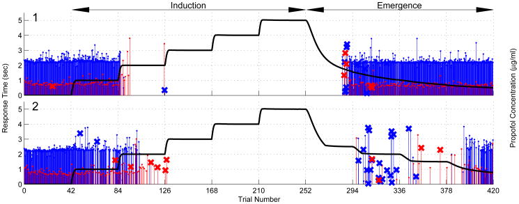
During induction, we increased the infusion rate of the computer-controlled pump to achieve the target effect-site concentrations (Purdon et al., 2013) in stepwise levels of 0, 1, 2, 3, 4, and 5 μg/ml every 14 minutes (Fig. 1, Induction) based on the Schnider pharmacokinetics model (Shafer and Gregg, 1992; Schnider et al., 1998). The effect site concentration is the concentration of propofol estimated to be in the brain area responsible for the observed behavioral or electrophysiological responses based on the pharmacokinetics model. We defined the target effect-site concentration at which the subject stopped responding as C_LOR (loss of response). For emergence, we used an adaptive dosing strategy. Beginning at the end of the 5 μg/ml level, we reduced the propofol concentration in a stepwise fashion to concentrations of C_LOR – 0.5 μg/ml, C_LOR – 1.0 μg/ml, C_LOR – 1.5 μg/ml and 0 μg/ml for 14 minutes each (Fig. 1, Emergence). Button press times were recorded throughout the experiment. The entire experiment lasted approximately 150 minutes.

Figure 1.

Target effect-site propofol concentration levels (black) and behavioral responses of verbal (subject's name and neutral words) stimuli (red) and auditory click stimuli (blue) for Subjects 1 (upper panel) and 2 (lower panel). Stimuli were delivered every four seconds. The heights of the vertical lines are the response times in seconds. An X at the tip of the line indicates an incorrect response whereas no X at the tip indicates a correct response. Absence of a vertical line indicates no response. Subject 1 had a low C_LOR, as a result, the predicted effect-site concentration did not decrease as fast as the target propofol concentration and did not show a stepwise fashion.

2.2. State-Space Model for Verbal Stimuli

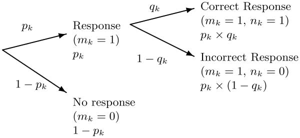
A state-space model consists of two components: the observation model and the state model. We first define the observation model for the responses to the verbal stimuli. Assume that the experiment consists of K verbal stimulus trials. On any trial there are three possible outcomes for the response to the verbal stimulus; the subject may respond correctly, respond incorrectly or not respond. Let m_k = 1 if the subject responds on trial k and 0 otherwise. If there is a response on trial k, let n_k = 1 if it is correct and 0 otherwise. Let p_k denote the probability of a response on trial k, i.e. that m_k = 1, and let q_k denote the probability of a correct response, i.e. n_k = 1. The observed data at trial k are the pair (m_k, n_k) which can assume the values {(1, 1), (1, 0), (0, 0)}. The observation model at trial k is therefore

$$\text{Pr}(m_k,n_k|p_k,q_k)={\left[p_k{(q_k)}^{n_k}{(1-q_k)}^{1-n_k}\right]}^{m_k}{(1-p_k)}^{1-m_k}$$ (1)

where we define p_k and q_k in terms of the cognitive state variables by the logistic relations

$$p_k={[1+exp(-x_k)]}^{-1}$$ (2)

$$q_k={[1+exp(-z_k)]}^{-1}.$$ (3)

It follows that p_k·q_k is the probability of a correct response at trial k (Fig. 2). We use p_k to define loss and recovery of consciousness, whereas p_kq_k can be used to define level of sedation. We define the state model for the unobservable cognitive state variables as the random walk equations

Figure 2.

Probability tree showing the three possible outcomes in response to a verbal stimulus at trial k.

$$x_k=x_{k-1}+{∊}_k$$ (4)

$$z_k=z_{k-1}+{\eta }_k$$ (5)

where ∊_k and η_k are zero-mean Gaussian random variables with variances ${\sigma }_{∊}^2{\mathrm{\Delta }}_k$ and ${\sigma }_{\eta }^2{\mathrm{\Delta }}_k$, where Δ_k is the time elapsed between verbal stimulus trials k − 1 and k.

Formulating the probability of response and the conditional probability of a correct response on each trial as a logistic function of the cognitive state variable ensures that these probabilities are properly defined between 0 and 1. The state-model provides a continuity constraint so that the current cognitive state and hence, the probability of a response and the conditional probability of a correct response depend on the previous cognitive state and experience. We let $\theta =\{{\sigma }_{∊}^2,{\sigma }_{\eta }^2,x_0,z_0\}$ denote the unknown parameters to be estimated.

2.3. State-Space Model for Click Stimuli

We can use the same logic presented for the verbal stimuli to develop a state-space model for the clicks. The only exception is we rewrite the observation equation to allow for four click stimuli presentations per trial: for each verbal stimulus, there are four click stimuli. Hence the observation model for the clicks is

$$\text{Pr}(m_k,n_k|p_k,q_k,4)=(\begin{array}{c}4\\ m_k\end{array}){(p_k)}^{m_k}{(1-p_k)}^{4-m_k}\times (\begin{array}{c}{m}_k\\ n_k\end{array}){(q_k)}^{n_k}{(1-q_k)}^{m_k-n_k}$$ (6)

where m_k = 0, 1, 2, 3, 4 is the number of responses and n_k = 0, 1, 2, …, m_k is the number of correct responses to the click stimuli, otherwise p_k, q_k, x_k and z_k are defined exactly as they were defined for the verbal state-space model. These are 15 possible outcomes in an any click trial block. The unknown parameters are again $\theta =\{{\sigma }_{∊}^2,{\sigma }_{\eta }^2,x_0,z_0\}$.

2.4. Model Estimation

Our objective is to develop a Bayesian procedure for model parameter estimation. We assume that there is a 2-dimensional state-space model for the verbal responses and a separate 2-dimensional state-space model for the click stimuli. We denote the unobserved state as X = (x_v,1, …, x_v,K, z_v,1, …, z_v,K, x_c,1, …, x_c,K, z_c,1, …, z_c,K), the model parameters as Θ = (θ_v, θ_c) and the, observed data as M = (m_v,1, …, m_v,K, n_v,1, …, n_v,K, m_c,1, …, m_c,K, n_c,1, …,n_c,K), where the subscripts v and c have been added to denote the verbal and click components of the model respectively. If we assume that f (Θ) is a prior distribution for Θ, then by Bayes' rule the posterior distribution for the parameters and the states is

$$f(\mathit{X},\mathbf{\Theta }|\mathit{M})=\frac{f(\mathit{M}|\mathit{X},\mathbf{\Theta })f(\mathit{X}|\mathbf{\Theta })f(\mathbf{\Theta })}{f(\mathit{M})}.$$ (7)

The observation models (Eqs. 1-3, 6) define f (M|X, Θ) and the state-space models (Eqs. 4-5) define f (X|Θ) and f (M) is the normalizing constant. To specify f(Θ) we chose the independent prior distributions for x_v,0, z_v,0, x_c,0 and z_c,0 to be uniform distributions each on the interval [0, 100]. For each of the variance parameters ${\sigma }_{∊,v}^2$, ${\sigma }_{\eta ,v}^2$, ${\sigma }_{∊,c}^2$ and ${\sigma }_{\eta ,c}^2$ we take as the prior distribution independent inverse gamma distributions with parameters α = 5 and λ = 1. These choices of prior distributions constrain the parameter estimation while allowing the shape of the posterior distribution to be determined by the likelihood.

We used the WinBUGS software (Lunn et al., 2000; Smith et al., 2009) to compute by Bayesian Monte Carlo methods the posterior densities f(X, Θ|M) and the marginal posterior densities of the form

$$f(x_{c,k}|\mathit{M})={\iint }_{\mathbf{\Theta }}f(\mathit{X},\mathbf{\Theta }|\mathit{M})\mathrm{d}\mathbf{\Theta }\mathrm{d}{\mathit{X}}_{[\mathit{c},\mathit{k}]},$$ (8)

where the inner integral is over the components of all values of Θ and the outer integral is over all components of X excluding x_c,k. We computed the comparable marginal posterior densities for z_c,k, x_v,k, z_v,k and for each component of Θ. We report the median of each marginal posterior density as the estimate of a given state at a particular trial and a given parameter. We report the uncertainty in any state or parameter estimate as the 95% or 90% credibility interval based on the Monte Carlo samples. The posterior densities were computed using 100,000 iterations after a 20,000 iteration burn-in period.

2.5. Model Selection

An important objective of our analysis is to understand how stimulus saliency affects the definitions of loss and recovery of consciousness during general anesthesia. Therefore, we analyzed the data with three different formulations of the state-space model to determine which gave the most parsimonious data descriptions. In Model A we assume a 4-dimensional state-space model as described in 2.2. That is, at each trial k there is a cognitive state x_v,k for the verbal stimuli and a cognitive state x_c,k for the click stimuli governing the subject's propensity to respond. There are also cognitive states z_v,k and z_c,k for the verbal and click stimuli respectively, governing the subject's conditional probability of responding correctly to each. Model B is the 3-dimensional special case of Model A which assumes that x_v,k = x_c,k, i.e. the probability of responding is the same for both stimulus types. Model C is another 3-dimensional special case of Model A. It assumes that z_v,k = z_c,k, i.e., the probability of correctly responding given that the subject responded is the same for both stimulus types.

To guide selecting among the 3 different models we computed for each the Deviance Information Criterion (DIC), which is an approximate Bayesian analogue of Akaike's Information Criterion used in likelihood analyses (Spiegelhalter et al., 2002). It is defined as

$$\text{DIC}=-2logf(\mathit{M}|\overline{\mathbf{\Theta }})+2(\overline{D}-\widehat{D})$$ (9)

where Θ̄ is the posterior mean of Θ, D̄ is the posterior mean of the deviance and D̂ = −2 log f (M|Θ̄) + 2 log h (M), where h(M) is the evidence, which can be, and is usually, set to equal 1 (Celeux et al., 2006). The second term in (9) defines the approximate number of parameters in the model, by analogy with AIC. The model with the smallest DIC is the one that would predict best a replicate set of data with the same structure observed in the current data. In this case, the model with the smallest DIC value would be preferred.

3. Results

3.1. Model Selection and Analyses of Individual Responses

We show in Fig. 1 the propofol target effect site concentrations and the behavioral responses for Subjects 1 (upper panel) and 2 (lower panel). Both subjects responded to all of the auditory stimuli at level 0 when no propofol was administered. During induction Subject 1 (Subject 2) stopped responding to the auditory stimuli at target propofol levels of 2 μg/ml (3 μg/ml), which we defined as the subject's C_LOR. Both subjects stopped responding to the clicks before the verbal stimuli. On emergence both subjects began responding when the target propofol level fell below C_LOR. Once Subject 1 began responding during emergence, he responded immediately and correctly to every stimulus. In contrast, Subject 2 did not respond consistently during emergence until the target level was 0.

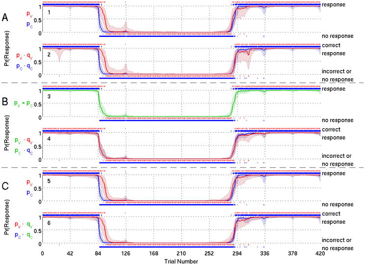
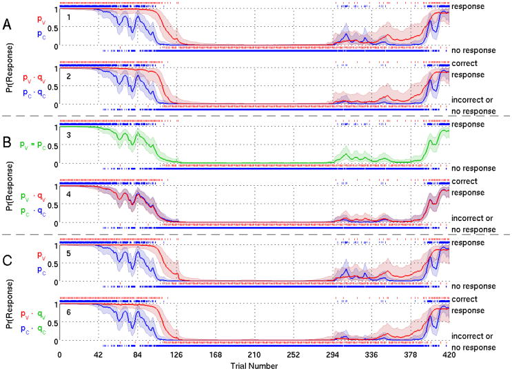
For Subjects 1 and 2 we show respectively in Figs. 3 and 4, the probability curve estimates from Model A (panels 1-2), Model B (panels 3-4) and Model C (panels 5-6). Model A estimates a distinct probability of response (Figs. 3 and 4, panel 1) and probability of correct response (Figs. 3 and 4, panel 2) for each of the two stimuli. In Model B, the common probability of a response curve (Figs. 3 and 4, panel 3) is similar in shape to the probability of the response to the click in Model A (Figs. 3 and 4, panel 1) because there are four times as many click stimuli (1680 presentations) as verbal stimuli (420 presentations). For the same reason, the two curves for the probability of a correct response (Figs. 3 and 4, panel 4) resemble the probability of a correct response for the clicks in Model A (Figs. 3 and 4, panel 2). The assumption of a common response probability for both types allows the click stimuli to determine the structure of both the probability of a response and the probability of a correct response.

Figure 3.

Model Fit Results for Subject 1 for Model A (panels 1-2), Model B (panels 3-4), Model C (panels 5-6). We show the marginal posterior median estimate of (solid curve) and 95% credible interval (shaded area) of the probability of a response (panels 1, 3 and 5) and probability of a correct response (panels 2, 4 and 6) to verbal stimuli and click stimuli. Response probability curves for verbal stimuli are red and for click stimuli are blue. Green curve (panel 3) indicates response probability curve estimated to be the same for verbal and click stimuli. A vertical dash above (below) the probability curves indicates a response (no response) to an auditory stimulus for panels 1, 3 and 5, or a correct response (an incorrect response or no response) for panels 2, 4 and 6.

Figure 4.

Model Fit Results for Subject 2 for Model A (panels 1-2), Model B (panels 3-4), Model C (panels 5-6). We show the marginal posterior median estimate of (solid curve) and 95% credible interval (shaded area) of the probability of a response (panels 1, 3 and 5) and probability of a correct response (panels 2, 4 and 6) to verbal stimuli and click stimuli. Response probability curves for verbal stimuli are red and for click stimuli are blue. Green curve (panel 3) indicates response probability curve estimated to be the same for verbal and click stimuli. A vertical dash above (below) the probability curves indicates a response (no response) to an auditory stimulus for panels 1, 3 and 5, or a correct response (an incorrect response or no response) for panels 2, 4 and 6.

For Model C, the response probability (Figs. 3 and 4, panel 5) is similar to Model A (Figs. 3 and 4, panel 1). The probability of correct response (Figs. 3 and 4, panel 6) is also similar to Model A (Figs. 3 and 4, panel 2), with a reduced probability of correct response for the verbal stimuli. Model C shows that assuming a common probability of a correct response for both types of stimuli yields a different probability of a response and probability of a correct response for each of the two stimuli.

The DIC analyses are summarized in Table 1 for the fits of Models A, B and C for all 10 subjects. In terms of minimum DIC, Model B is not preferred for any subject, if we use the criterion of a DIC difference of at least 5. Model B has the lowest DIC only for subject 6 (346.6), yet this is not appreciably different from the DIC value for Model C (349.5). Model A is the preferred model for subjects 1, 4, and 10 whereas Model C is the preferred model for subjects 8 and 9. The DICs for Models A and C are sufficiently close (< 5) that we consider these models indistinguishable for subjects 2, 3, 5 and 7. Therefore, our results suggest that either a model assuming 4 distinct cognitive states, Model A, or a reduced model assuming that the conditional probabilities of response of response are the same for verbal and click stimuli, Model C, would be preferred. That Models A and C would be the preferred models was suggested by the analyses of the data from subjects 1 and 2 which showed that unlike Model B, these former two models preserved the response characteristics of the two different stimuli.

Table 1.

Comparison of Deviance Information Criterion for Models A, B and C for all Ten Subjects.

Subject	1	2	3	4	5	6	7	8	9	10
Model A	257.7	660.2	393.3	788.8	677.9	353.2	995.6	648.9	550.8	839.3
Model B	294.0	758.7	479.8	827.0	863.7	346.4	1036.0	768.1	552.0	857.5
Model C	269.3	660.4	388.8	804.1	675.7	349.5	996.0	641.2	542.9	855.3

Bold values indicate the preferred model(s) for the subject in terms of minimum DIC.

Our analyses using both Models A and C showed that the verbal probability of a correct response curve tended to be above the click probability of a correct response curve for nearly all trials for all of the subjects. This suggested that the loss of responsiveness to the less salient clicks occurred before loss of responsiveness to the more salient verbal stimuli. Similarly responsiveness to the verbal stimuli returned prior to the return of the responsiveness to the click stimuli. Therefore, for each subject we defined the point of loss of consciousness (LOC) as the time at which the probability of a correct response to a verbal task was less than 0.05 and remained so for at least 10 minutes. Similarly, we defined recovery of consciousness (ROC) as the first time, since being unconscious, at which the probability of a correct response to a verbal task was greater than 0.05 and remained so for at least 10 minutes.

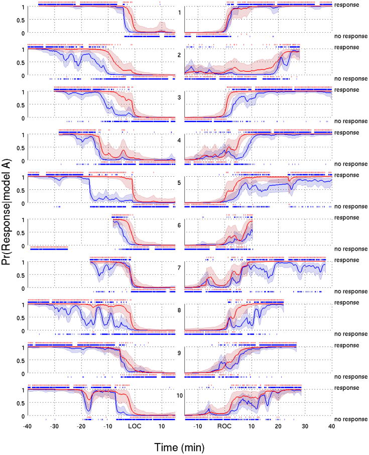
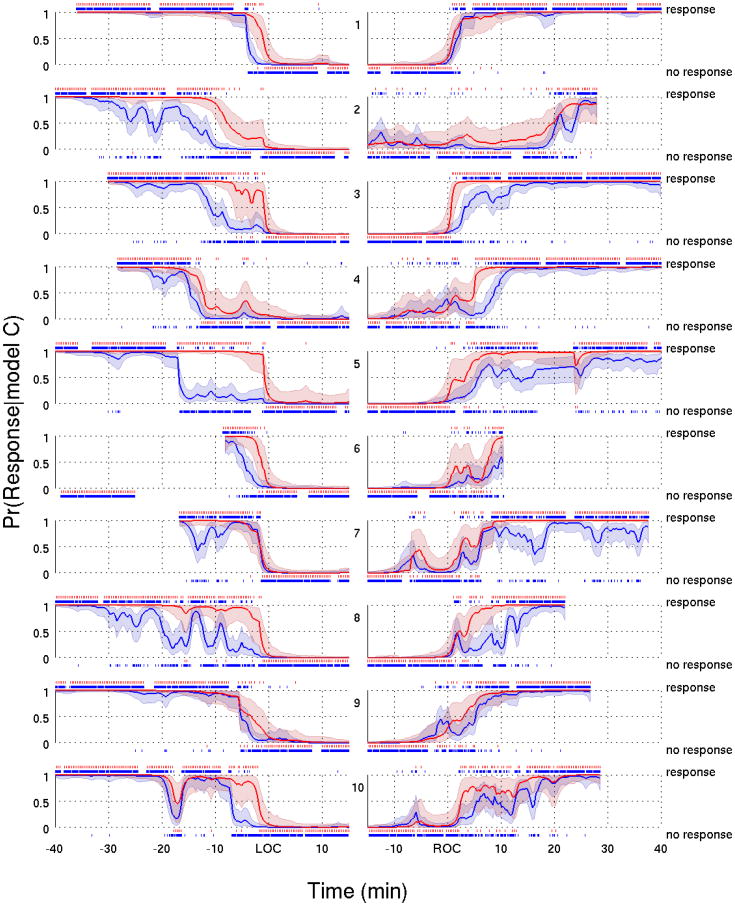
For Model A (Fig. 5) and C (Fig. 6) we plotted the fits of the data from all of the subjects aligned with respect to LOC and with respect to ROC. Both models give similar estimates of both response probability curves. For each subject, the tendency of the click response probability curve to decline before and increase after the verbal response probably curve is evident for Model A (Fig. 5) and Model C (Fig. 6). The difference between these curves during induction defines a transition into loss of consciousness, whereas the difference on emergence defines a transition through recovery of consciousness.

Figure 5.

Response probability curves for the verbal (red) and click (blue) stimuli with their associated 95% credible intervals based on Model A for all ten subjects during the transition into loss of consciousness (left panels) and into recovery of consciousness (right panels). A vertical dash above (below) the probability curves indicates a response (no response) to an auditory stimulus. All probability curves in the left (right) panels were aligned with respect to LOC (ROC).

Figure 6.

Response probability curves for the verbal (red) and click (blue) stimuli with their associated 95% credible intervals based on Model C for all ten subjects during the transition into loss of consciousness (left panels) and into recovery of consciousness (right panels). A vertical dash above (below) the probability curves indicates a response (no response) to an auditory stimulus. All probability curves in the left (right) panels were aligned with respect to LOC (ROC).

3.2. Analyses of Pooled Behavioral Responses

To develop an average estimate of these transitions we fit both Models A and C to the pooled data. We used both Models A and C to conduct the pooled analysis because the DIC values (Table 1) and fits of the two were indistinguishable. We aligned the verbal and click responses across all 10 subjects separately with respect to LOC and with respect to ROC. In each 20-second bin-the time required to present four click stimuli and one verbal stimulus-we tallied the number of stimuli, the number of responses and the number of correct responses for the 10 subjects. For Model A the verbal stimuli observation model (Eq. 1) became a binomial model with n = 10, whereas the clicks observation model is a binomial in Eq. 6 with n = L_k instead of 4, where L_k is the number of trials aligned at a given time. The maximum of L_k is 40 and the minimum 4. The state equation is 4-dimensional for Model A. The observation models for Model C are the same as for Model A. The state equation for Model C is again 3-dimensional as in the individual analyses. We used the Bayesian Monte Carlo methods to fit both models to the pooled data aligned with respect to LOC and with respect to ROC.

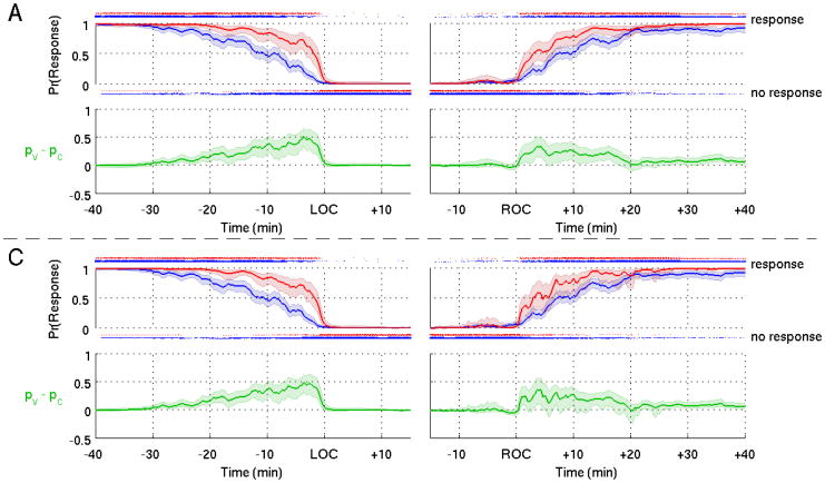
The pooled verbal (Fig. 7, red curves) and click (Fig. 7 blue curves) response probability curves and their difference curve (Fig. 7 green curves) computed from Model A (Fig. 7 upper panels) and C (Fig. 7 lower panels) agreed closely. The pooled probability response curves computed from both Models A and C (Fig. 7) show clearly the tendency to lose responsiveness to the more salient verbal stimuli (Fig. 7, red curves) later and regain responsiveness to them sooner relative to the less salient click stimuli (Fig. 7, blue curves). This tendency is also evident in the difference curves (Fig. 7, green curves). The fact that during induction the lower bound of the 95% credibility interval for the difference curves lies above zero for the entire twenty minutes prior to LOC suggests that the click probability response curve is significantly greater than the verbal probability response curve. During emergence the lower bound of the 95% credibility intervals for the difference curves lies above zero for the entire twenty minutes following ROC suggesting that the click probability response curve is again significantly greater than the verbal probability response curve. These findings demonstrate that stimulus saliency is important for defining the transitions into and recovery from unconsciousness induced by general anesthesia.

Figure 7.

Group level response probability curves for the verbal (red) and click stimuli (blue) and the differences in the curves (green) with their associated 95% credible intervals (shaded areas) for loss of consciousness (left panels) and recovery of consciousness (right panels) computed from Models A (upper four panels) and C (lower four panels). Dots above (below) the probability curves indicate a response (no response) to an auditory stimulus.

4. Discussion and Conclusion

We have studied the use of state-space models fit by Bayesian Monte Carlo methods to analyze the effect of stimulus saliency for defining loss and recovery of consciousness under general anesthesia. We used DIC to aid in model selection. Because no single model gave a superior description of the data for all of the study subjects, we used two models to analyze the data for the individual subjects and to conduct the pooled analyses across subjects. Our results show that during induction subjects tend to lose their responsiveness to less salient auditory clicks before losing their responsiveness to the more salient verbal stimuli neutral words and the subject's name. During emergence subjects tend to regain their responsiveness to the more salient verbal stimuli before regaining responsiveness to the less salient auditory clicks. We conclude that taking account of stimulus salience is important for understanding how to define loss and recovery of consciousness under general anesthesia.

Our experimental paradigm offers improvements over current experimental approaches to characterizing loss of consciousness, recovery of consciousness and unconsciousness induced by general anesthesia (Chernik et al., 1990; Kearse et al., 1998). We used a computer controlled system to deliver precisely timed stimuli and to record the subjects' responses. Our stimuli consisted of auditory clicks at two different frequencies (40 Hz and 84 Hz) and verbal stimuli consisting of the subject's name and neutral words. We chose the subject's name as a stimulus because it is among the most salient auditory stimuli that could be administered. Moreover, anesthesiologists frequently address patients by their preferred names during emergence from general anesthesia because of their presumed saliency. By administering in an interleaved manner salient and non-salient stimuli we were able to demonstrate that stimulus saliency is important for defining be-haviorally the onset and offset of unconsciousness during general anesthesia. In our study, we treated the neutral words and the subject's name as a single stimulus type because our preliminary analyses showed the subject's responses to these stimuli could not be distinguished. We also treated the two frequencies for the verbal stimuli as a single stimulus. In future work, we will report on the relationship between the differences in the electroencephalogram responses of these subjects to the two different auditory stimuli.

The current state-space model is an extension of previous models used to analyze learning and behavioral performance (Smith et al., 2004, 2005, 2009). In previous applications of the state-space paradigm, the study needed only to consider whether the response was correct or incorrect on each trial because the subject was certain to respond on each trial with probability one. In contrast, in this study which required our subjects to execute the behavioral task while receiving increasing and then decreasing doses of propofol, the probability of responding on each trial was not one. This key feature of the responses was easily accounted for by using a two-stage formulation of the responses for both the verbal and click stimuli. The first stage considers the probability of a response whereas the second stage considers the probability of a correct response given that the subject responded (Fig. 2).

To accommodate the two-stage nature of the subject responses, we specified in the state equation a cognitive state variable for each of the two response components. Earlier applications of the state-space paradigm used maximum likelihood approaches computed with an approximate EM algorithm (Smith et al., 2004). Under the EM framework, a new algorithm has to be written for each model making its use less feasible when model selection is central to the analysis. By using the Bayesian Monte Carlo methods implemented in WinBUGS to conduct the analysis we only needed to specify the observation and state equations for each new model (Lunn et al., 2000; Smith et al., 2009), WinBUGS used a Bayesian Monte Carlo scheme to conduct the model analysis thus, obviating the need to write a fitting algorithm for each model.

To conduct our group analyses, we aligned the data across subjects with respect to LOC and ROC because these time points have the same behavioral interpretation for each subject. In contrast, the more traditional approach of constructing a Bayesian hierarchical model (Gelman et al., 1995; Smith et al., 2005) to exchange information among subjects to estimate simultaneously individual and population response curves and then determine individual and population LOC and ROC would not be accurate. This is because the cognitive state dynamics around LOC and ROC differ appreciably across subjects. Moreover, in our analyses of the neurophysiological data from this study, we use LOC and ROC to align the spectrograms across subjects (Purdon et al., 2013). Use of similar strategies to align data across subjects with respect to estimated reference points is a common practice in circadian rhythm studies (Czeisler et al., 1989).

We used DIC to help guide our selection among the three models not to identify a “true model”. DIC is known to be problematic in state space models as the effective number of parameters (D̄ − D̂ in Eq. 9) can be negative (Celeux et al., 2006). This was not an issue in any of our experiments. By this criterion, Model B was the least favored whereas Models A and C were essentially comparable, with Model C being the more parsimonious of the two. Both Models A and C suggest that the probability of responding to the verbal stimuli and the probability of responding to the click stimuli are different. This is consistent with the idea that the verbal stimuli, in particular the subject's name are more salient whereas the click stimuli are less salient. Being more parsimonious, Model C suggests that the probability of a correct response for the two types of stimuli do not differ. Hence, this study provides evidence that the propensity to respond to the two types of stimuli differs yet, it is less clear that the conditional probability of correct responses differs for the two stimuli.

Our work suggests that behavioral markers can be developed to define the points of loss and recovery of consciousness due to administration of anesthetic agents. The behavioral markers must now be related to neurophysiological markers such as EEG changes associated with different stages of general anesthesia (Brown et al., 2010; Purdon et al., 2013) to gain a more accurate systems neuroscience characterization of the transitions into and out of unconsciousness induced by an anesthetic such as propofol. We used propofol in our experiments because it is the most widely used anesthetic agent. Our experimental and state-space analysis paradigms can be readily adapted to characterize loss and recovery of consciousness during induction and emergence from other anesthetics. Similarly, because p_kq_k defines the probability of a correct response, it can be used to define quantitatively the concept of level of sedation in terms of different stimulus types. In addition to the time series of binary responses, we recorded for each stimulus presentation the subject's reaction times. These data can be analyzed separately or jointly with the binary responses to gain a more complete picture of how behavioral responses are affected by general anesthesia (Prerau et al., 2009). These experiments and analyses will be the topics of future investigations.

Highlights.

• We study induction and emergence from propofol-induced loss of consciousness.

• We have subjects execute two interleaved computer delivered behavioral tasks.

• We fit the model to the experimental data using Bayesian Monte Carlo methods.

• Our analysis provides a principled approach for defining loss and recovery of consciousness.

References

- Alkire MT, Haier RJ, Fallon JH. Toward a unified theory of narcosis: brain imaging evidence for a thalamocortical switch as the neurophysiologic basis of anesthetic-induced unconsciousness. Conscious and Cogn. 2000;9:370–386. doi: 10.1006/ccog.1999.0423. [DOI] [PubMed] [Google Scholar]
- Brown EN, Lydic R, Schiff ND. General anesthesia, sleep, and coma. N Engl J Med. 2010;363:2638–2650. doi: 10.1056/NEJMra0808281. [DOI] [PMC free article] [PubMed] [Google Scholar]
- Celeux G, Forbes F, Robert CP, Titterington DM. Deviance information criteria for missing data models. Bayesian Anal. 2006;1:651–674. [Google Scholar]
- Chernik DA, Gillings D, Laine H, Hendler J, Silver JM, Davidson AB, Schwam EM, Siegel JL. Validity and reliability of the observer's assessment of alertness/sedation scale: study with intravenous midazolam. J Clin Psychopharmacol. 1990;10:244–251. [PubMed] [Google Scholar]
- Czeisler CA, Kronauer RE, Allan JS, Duffy JF, Jewett ME, Brown EN, Ronda JM. Bright light induction of strong (type 0) resetting of the human circadian pacemaker. Science. 1989;244:1328–1333. doi: 10.1126/science.2734611. [DOI] [PubMed] [Google Scholar]
- Gelman A, Carlin JB, Stern HS, Rubin DB. Bayesian data analysis. Chapman and Hall; 1995. [Google Scholar]
- Kearse LA, Rosow C, Zaslavsky A, Connors P, Dershwitz M, Denman W. Bispectral analysis of the electroencephalogram predicts conscious processing of information during propofol sedation and hypnosis. Anesthesiol. 1998;88:25–34. doi: 10.1097/00000542-199801000-00007. [DOI] [PubMed] [Google Scholar]
- Lunn DJ, Thomas A, Best N, Spiegelhalter D. WinBUGS - a bayesian modelling framework: concepts, structure, and extensibility. Stat and Comp. 2000;10:325–337. [Google Scholar]
- Prerau MJ, Smith AC, Eden UT, Kubota Y, Yanike M, Suzuki W, Graybiel AM, Brown EN. Characterizing learning by simultaneous analysis of continuous and binary measures of performance. J Neurophysiol. 2009;102:3060–3072. doi: 10.1152/jn.91251.2008. [DOI] [PMC free article] [PubMed] [Google Scholar]
- Purdon PL, Pierce ET, Mukamel EA, Prerau MJ, Walsh JL, Wong KFK, Salazar-Gomez AF, Harrel PG, Sampson A, Cimenser A, Ching S, Kopell N, Tavares-Stoeckel CL, Habeeb K, Merhar R, Brown EN. Electroencephalogram signatures of loss and recovery of consciousness from propofol. PNAS. 2013;110:1142–1151. doi: 10.1073/pnas.1221180110. [DOI] [PMC free article] [PubMed] [Google Scholar]
- Schnider TW, Minto CF, Gambus PL, Andresen C, Goodale DB, Shafer SL, Youngs EJ. The influence of method of administration and covariates on the pharmacokinetics of propofol in adult volunteers. Anesthesiol. 1998;88:1170–1182. doi: 10.1097/00000542-199805000-00006. [DOI] [PubMed] [Google Scholar]
- Shafer SL, Gregg KM. Algorithms to rapidly achieve and maintain stable drug concentrations at the sit of drug effect with a computer-controlled infusion pump. J Pharmacokinet Pharmacodyn. 1992;20:147–169. doi: 10.1007/BF01070999. [DOI] [PubMed] [Google Scholar]
- Smith AC, Frank LM, Wirth S, Yanike M, Hu D, Kubota Y, Graybiel AM, Suzuki WA, Brown EN. Dynamic analysis of learning in behavioral experiments. J of Neurosci. 2004;24:447–461. doi: 10.1523/JNEUROSCI.2908-03.2004. [DOI] [PMC free article] [PubMed] [Google Scholar]
- Smith AC, Shah SA, Hudson AE, Purpura KP, Victor JD, Brown EN, Schiff ND. A Bayesian statistical analysis of behavioral facilitation associated with deep brain stimulation. J Neurosci Methods. 2009;183:267–276. doi: 10.1016/j.jneumeth.2009.06.028. [DOI] [PMC free article] [PubMed] [Google Scholar]
- Smith AC, Stefani MR, Moghaddam B, Brown EN. Analysis and design of behavioral experiments to characterize population learning. J Neurophysiol. 2005;93:1776–1792. doi: 10.1152/jn.00765.2004. [DOI] [PubMed] [Google Scholar]
- Spiegelhalter DJ, Best NG, Carlin BR, van der Linde A. Bayesian measures of model complexity and fit. J R Stat Soc Ser B. 2002;64:583–616. [Google Scholar]
- Wirth S, Yanike M, Frank LM, Smith AC, Brown EN, Suzuki WA. Single neurons in the monkey hippocampus and learning of new associations. Science. 2003;300:1578–1584. doi: 10.1126/science.1084324. [DOI] [PubMed] [Google Scholar]