Abstract
Accurate automated segmentation and detection of ovarian cancer metastases may improve the diagnosis and prognosis of women with ovarian cancer. In this paper, we focus on an important subset of ovarian cancer metastases that spread to the surface of the liver and spleen. Automated ovarian cancer metastasis detection and segmentation are very challenging problems to solve. These metastases have a wide variety of shapes and intensity values similar to that of the liver, spleen and adjacent soft tissues. To address these challenges, this paper presents a variational approach, called tumor sensitive matching flow (TSMF), to detect and segment perihepatic and perisplenic ovarian cancer metastases. TSMF is an image motion field that only highlights metastasis-caused deformation on the surface of liver and spleen while dampening all other image motion between the patient image and the atlas image. It provides several benefits: 1) juxtaposing the roles of image matching and metastasis classification within a variational framework; 2) only requiring a small set of features from a few patient images to train a metastasis-likelihood function for classification; and 3) dynamically creating shape priors for geodesic active contour (GAC) to prevent inaccurate metastasis segmentation. We compared the TSMF to an organ surface partition (OSP) baseline approach. At a false positive rate of 2 per patient, the sensitivities of TSMF and OSP were 87% and 17% (p < 0.001), respectively. In a comparison of the segmentations conducted using TSMF-constrained GAC and conventional GAC, the volume overlap rates were 73±9% and 46±26% (p < 0.001) and average surface distances were 2.4±1.2mm and 7.0±6.0mm (p < 0.001), respectively. These encouraging results demonstrate that TSMF could accurately detect and segment ovarian cancer metastases.
Keywords: Ovarian Cancer Metastases, Tumor Sensitive Matching Flow, Dynamic Shape Prior, Level Set
1. Introduction
Approximately 22,240 new cases and 14,030 deaths are predicted to occur from ovarian cancer in the United States in 2013 (NCI, 2013). Ovarian cancer has a high mortality rate and 69% of women with ovarian cancer will succumb to the disease (Lengyel, 2010). The high mortality is mainly caused by a genetically unstable carcinoma that metastasizes rapidly (Cancer-Genome-Atlas-Research-Network, 2011). The high death-rate is also explained by the fact that as many as 75% of patients already have metastases to the pelvis and upper abdomen at the time of initial diagnosis because patients are often asymptomatic until the cancer has already spread widely (Lengyel, 2010; Memarzadeh and Berek, 2001). Accurate detection and segmentation of ovarian cancer metastases thus have potentially great clinical impact on improving the prognosis and treatment of women with ovarian cancer.
Computer-aided diagnosis and medical image analysis unfortunately place little emphasis on ovarian cancer imaging despite urgent clinical demands. Existing research (Chen et al., 2009; Krivanek and Sonka, 1998) on ovarian imaging has focused on segmenting ovarian follicles from ultrasound images for infertility treatment. Microarray images are primary data sources for early detection and segmentation of ovarian-cancer related epithelial cells, stroma, or vascular markers from ovary tissue samples (Janowczyk et al., 2009; Signolle et al., 2008). In this paper, we focus on detecting and segmenting perihepatic and perisplenic ovarian cancer metastases (outside and adjacent to liver and spleen) on contrast-enhanced CT images, two common locations of ovarian cancer metastases in the peritoneum and presenting in approximately 70% of patients at the time of initial diagnosis (Nougaret et al., 2012).
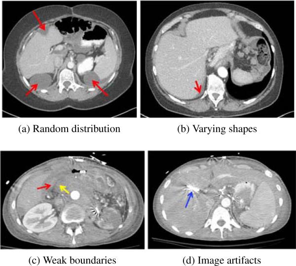
However, detection and segmentation of ovarian cancer metastases pose substantial challenges (Fig. 1). Most computer-aided diagnosis methods (Doi, 2007; Hong et al., 2000; Linguraru et al., 2012b) are developed for the detection of tumors growing inside the organs. On the contrary, ovarian cancer metastases can spread randomly throughout the peritoneum, a potential space in the abdomen and pelvis. Two common locations of spread are to the liver and spleen (Fig. 1a). The metastases can have a wide variety of shapes, e.g., elongated (Fig. 1b) and spherical (Fig. 1a), which prevents discriminative shape descriptors (Sundaram et al., 2007) from reliably detecting and segmenting them. Accurate metastasis segmentation is also nontrivial due to weak boundaries of low contrast between metastases and surrounding tissues (Fig. 1c). Image artifacts further complicate the metastasis segmentation (Fig. 1d).
Figure 1.
Challenges of detection and segmentation of ovarian cancer metastases (red arrows). (a) Random distribution in the abdomen, (a, b) varying metastasis shapes, e.g., elongated in (b) and spherical in (a), (c) weak boundaries of low contrast between metastases and surrounding tissues (yellow arrow), and (d) imaging artifacts caused by metallic streaks (blue arrow).
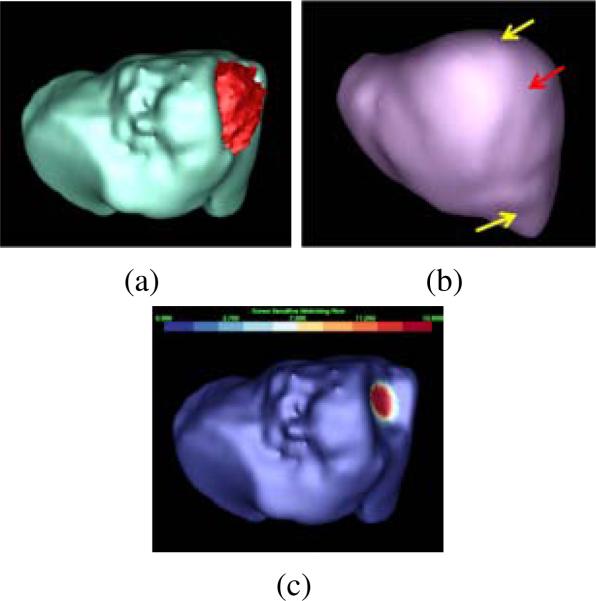
In our earlier work (Liu et al., 2012), we first presented a tumor sensitive matching flow (TSMF) method to detect and segment ovarian cancer metastases (Fig. 2). To search for randomly distributed metastases, TSMF computation juxtaposes the roles of metastasis classification/image matching between patient images and atlas images within a variational framework. TSMF vectors have the greatest magnitudes in metastasis regions and are suppressed in all other areas (Fig. 2c). Metastases are thus detected and segmented by searching for large TSMF vectors.
Figure 2.
Tumor sensitive matching flow (TSMF) for the detection and segmentation of ovarian cancer metastases. (a) A metastasis (red) attached to the liver (cyan), (b) the liver atlas (violet), and (c) TSMF results, where the magnitudes of flow vectors are mapped into the organ surface and blue to red represents small to large shape variance. The fundamental idea of the TSMF computation is to only highlight shape variance caused by metastases between the patient organ and the atlas (pointed by a red arrow in (b)), while all other shape variance due to individual difference (marked by yellow arrows) are suppressed. Metastases are thus be identified by searching for large TSMF vectors (red regions in (c)).
In this paper, we extend our earlier work in three ways. First, we augment the metastasis-likelihood function by using a Gaussian mixture model to describe metastasis intensity distribution and applying shape index to measure local shape variance. The enhanced metastasis-likelihood function leads to better TSMF computation and yields more accurate metastasis detection. Moreover, our metastasis-likelihood function only requires a small set of features from a few patient images due to our versatile framework that jointly performs image matching and metastasis classification. Second, we embed TSMF shape priors into the geodesic active contour (GAC) (Caselles et al., 1997), a level set framework, to segment metastases based on the observation that image regions with large TSMF vectors approximately represent metastasis shapes. Different from the conventional shape-constrained level set segmentation (Chan, 2005; Cremers et al., 2006), TSMF shape priors are dynamically constructed during the image matching process. TSMF shape priors are robust to the wide variety of metastasis shapes because they are always adaptable to the current patient. Therefore, TSMF-constrained GAC can generate accurate metastasis segmentation. Third, we extensively validate our algorithm on a test dataset with 108 patient images. We analyze the choice of key parameters in TSMF computation, the detection accuracy with respect to the metastasis size, the detection accuracy of perihepatic and perisplenic ovarian cancer metastases, the comparison between the TSMF method and a baseline organ surface partition (OSP) approach, as well as the segmentation accuracy comparison between the GAC and our TSMF-constrained GAC. All results demonstrated that TSMF method is an accurate approach to detect and segment ovarian cancer metastases.
2. Related Work
The purpose of TSMF computation is to identify metastasis-caused shape variance. Shape variance is measured in terms of image motion between the patient image and the atlas image, which is similar to optical flow computation except that TSMF only highlights metastasis-caused image motion. Large TSMF vectors indicate potential locations of perihepatic or perisplenic ovarian cancer metastasis candidates and facilitate detecting them. Hepatic tumor detection and segmentation are another important topic related to our work because we intend to detect perihepatic ovarian cancer metastases in this paper. However, hepatic tumor image analysis has in the past concentrated on finding tumors arising from within the liver itself, while our TSMF method detects ovarian cancer metastases growing along the liver surface. We also develop a TSMF-constrained GAC approach to segment metastases, which belongs to the domain of level set image segmentation. Thus, in this section, we review relevant work on optical flow computation, hepatic tumor analysis, and level set segmentation.
2.1. Optical Flow Computation
This section introduces the concept of optical flow and its recent development and application to medical image analysis. Optical flow (Lucas and Kanade, 1981; Horn and Schunck, 1981) is the distribution of moving velocities of intensity patterns. One fundamental assumption of optical flow computation is that the intensities of corresponding points are constant in two images. However, the intensity constancy model alone fails to estimate optical flow because a single equation established upon the intensity model cannot estimate multiple flow vector components. This issue is called the aperture problem (Horn and Schunck, 1981). Smoothness constraint is therefore introduced into optical flow computation, which assumes that flow vectors vary smoothly except at motion discontinuities. Optical flow is thus estimated by combining intensity constancy model and flow smoothness assumptions. Early optical flow methods (Black and Jepson, 1996; Lucas and Kanade, 1981; Singh, 1990) subdivided the image plane into several blocks and performed block-to-block image matching between two images assuming that optical flow vectors remain constant within an image block. However, the flow field is prone to inconsistency as well as over-smoothing at motion boundaries because the size of an image block is difficult to determine.
To avoid the size determination, Horn (Horn and Schunck, 1981) explicitly placed an intensity constancy model and a smoothness constraint into a variational functional. Minimizing the functional yields an optical flow field. Variational approaches not only allow the user to freely combine optical flow models within a functional, but also provide a solid mathematical theory, the so-called Euler-Lagrange equation, to minimize the functional. Thus, variational approaches have received great attention in optical flow computation. Brox (Brox et al., 2004) introduced a gradient constancy model into the variational framework and applied image warping techniques to generate accurate optical flow. Papenberg (Papenberg et al., 2006) compared different optical flow models in optical flow estimation, such as Laplacian constancy, Hessian norm constancy, and Hessian determinant constancy. Recently, Zimmer (Zimmer et al., 2011) developed a tensor representation to generally define the variational optical flow computation. Thorough surveys related to optical flow computation can be found in (Fleet and Weiss, 2005; Weickert et al., 2006).
Because optical flow can accurately represent image motion between two images, it has been widely applied to medical image registration (Dawood et al., 2008; Keeling and Ring, 2005), tracking (Linguraru et al., 2008; Liu et al., 2008), and colorectal polyp detection (Acar et al., 2001). Our TSMF method also exploited this beneficial property to identify metastasis-caused shape variance.
2.2. Hepatic Tumor Analysis
The liver is one of the most common sites of ovarian cancer metastases in the peritoneum. Many such metastases implant and grow on the liver surface (“perihepatic” metastases) (Figs. 1a and 1b). Hepatic tumors have the similar appearance to ovarian cancer metastases except that most of hepatic tumors are inside the liver. In this section, we describe hepatic tumor detection and segmentation, and point out the similarity and difference between these approaches and our TSMF method.
There is limited previous work on hepatic tumor detection (Doi, 2007) because hepatic tumors have low contrast intensity values with the normal liver tissue. Chen (Chen et al., 1998) used a deformable model to segment the liver on CT images, and employed neural network and texture features on the liver segmentation to identify tumors. Hong (Hong et al., 2000) employed adaptive thresholding to segment the liver and a Bayes classifier to detect spherical tumors at liver boundaries. Joshi (Joshi and Londhe, 2013) extended adaptive thresholding strategy to detect hepatic tumors inside the liver by performing region splitting and merging operations on the CT images. Multi-scale wavelet transform was used as texture features in (Mala et al., 2006), and experimental results indicated better detection accuracy due to the multi-scale property of texture features. Wu (Wu et al., 2013) developed a cascade learning method to detect hypodense and hyperdense liver lesions by concatenating multiple classifiers. Their method collected all information from the output from a given classifier as additional information for the subsequent classifier in the cascade to sequentially reduce false positives. A more sophisticated strategy was found in (Bilello et al., 2004), in which an adaptive thresholding algorithm was again used to identify interior hepatic lesion candidates followed by a sliding tangent circle algorithm to search for peripheral lesions. A quadratic fitting algorithm was then exploited to segment hepatic lesions which were further classified into cysts, metastases, and hemangiomas based on texture and shape information. Recent progress on liver tumor detection has shifted to taking advantage of high-quality CT imaging technologies, such as multiphase CT (Tateyama et al., 2011; Xu et al., 2011; Zhang et al., 2011).
Hepatic tumor segmentation is another important topic because accurate tumor segmentation is critical for the evaluation of tumor treatment (Tuma, 2006). In 2008, a competition of hepatic tumor segmentation was held in conjunction with the International Conference on Medical Image Computing and Computer Assisted Intervention (MICCAI) to encourage researchers to focus on hepatic tumor segmentation (Deng and Du, 2008). All CT images in the competition were collected with contrast enhancement, which aids in distinguishing tumors from healthy liver parenchyma. They were divided into training and testing datasets, and each of them was also provided with ground-truth for the titative evaluation. The quantitative evaluation. The workshop also gave five metrics to score the participated algorithms, including volume overlap, volume difference, absolute surface distance, squared surface distance, and maximum surface distance. One interactive, five semi-automatic and four automatic segmentation algorithms attended this competition. The highest score was achieved by the interactive segmentation algorithm, which employed graph cuts and watershed approaches (Stawiaski et al., 2008). Comparable scores were achieved by several semi-automatic segmentation algorithms, including a level set with fuzzy pixel classification (Smeets et al., 2008), adaptive thresholding and morphological processing (Moitz et al., 2008), and voxel classification and propagational learning (Zhou et al., 2008). The most successful automated segmentation algorithms were based on two machine learning techniques, cognition network (Schmidt et al., 2008) and ensemble segmentation using AdaBoost training (Shimizu et al., 2008).
Machine learning methods have become popular in recent work on hepatic tumor segmentation. Hame (Hame and Pollari, 2012) interactively classified CT images into tumor and non-tumor regions, and refined tumor regions using Hidden Markov fields. Support vector machine and affinity constraint propagation were explored to semi-automatically segment hepatic tumors in (Freiman et al., 2011). Recently, Linguraru (Linguraru et al., 2012b) developed a fully automated tumor segmentation algorithm by comparing the segmented liver with a sequence of liver atlases to identify tumors along liver boundaries through shape analysis. Hepatic tumors were segmented using machine learning with shape and intensity priors.
Nevertheless, the major difference between hepatic tumor analysis and our approach is that their methods aim to find hepatic tumors inside the liver while our work focuses on the detection of ovarian cancer metastases outside the liver and spleen. Detection and segmentation of perihepatic ovarian cancer metastasis in this paper also have some similarities to the identification of hepatic tumors on the liver boundaries (Hong et al., 2000; Bilello et al., 2004). However, in contrast to hepatic tumors which are often more spherical, ovarian cancer metastases manifest a wide variety of shapes (Figs. 1a and 1b), which prevents predefining metastasis shape priors in metastasis detection and segmentation. Moreover, ovarian cancer metastases often present weak boundaries with the liver, which easily fails the adaptive thresholding algorithm in hepatic lesions segmentation (Joshi and Londhe, 2013; Bilello et al., 2004).
2.3. Level Set Methods
In this section, we give an overview of level set methods because they are used to segment ovarian cancer metastases in this work. The level set method (Sethian, 1999) is a process of interface propagation by integrating image information into a partial-differential-equation (PDE) framework. The interface stops at the object boundaries and divides the image into several meaningful objects. The level set propagation has many beneficial properties, including high segmentation accuracy, simplified region representation, and accurate tracking of object topology changes. Therefore, the level set method is widely used in tumor segmentation (Linguraru et al., 1989; Sean et al., 2002; Smeets et al., 2010).
The level set method is generally classified into two categories, edge-based and region-based. The edge-based approaches (Caselles et al., 1997; Kichenassamy et al., 1996) extract objects by using image gradients to formulate the interface speed term. However, these methods are sensitive to the image noise and the level set interface is easily stuck at noisy image points. To address this issue, the region-based methods compute global region statistics and perform region competition to drive level sets (Mumford and Shah, 1989; Zhu and Yuille, 1996). The Chan-Vese model (Chan and Vese, 2001) is a typical region-based approach, in which the mean intensity difference between foreground and background forces the level set to stop at object boundaries. Kim (Kim et al., 2005) chose a non-parametrical distribution model to describe region statistics, which was demonstrated to produce more accurate segmentations than the Chan-Vese model. Brox (Brox and Weickert, 2006) extended two-region competition to simultaneously segment multi-objects. Paragios (Paragios and Deriche, 2002) combined edge-based and region-based level sets into a unified framework to take advantages from both sides, which claimed better performance than edge-based solely or region-based solely methods. The region-based level set can also include different visual cues, such as texture and image motion (Brox et al., 2010; Cremers et al., 2007), to assist image segmentation.
Recent research on level set segmentation has shifted to embedding shape priors into the segmentation framework because weak object boundaries ubiquitously exist. Cremers (Cremers et al., 2003) developed a dynamical labeling strategy to constrain the target object with a shape prior. Chan (Chan, 2005) introduced an affine registration process to align the shape prior with the target object. Cremers (Cremers et al., 2006) subsequently included this affine registration process into his early work (Cremers et al., 2003) to segment multiple objects using multiple shape priors. Instead of using Gaussian probability model to describe the shape prior, Dambreville (Dambreville et al., 2008) chose kernel PCA to delineate the distribution of shape priors. Recently, sparse coding (Prisacariu and Reid, 2011; Zhang et al., 2012) was studied to nonlinearly combine training shape priors to represent the target object, based on the assumption that training datasets are over-complete. However, these methods might not stably segment ovarian cancer metastases because the wide variety of metastasis shapes cannot be constructed beforehand.
3. Methodology
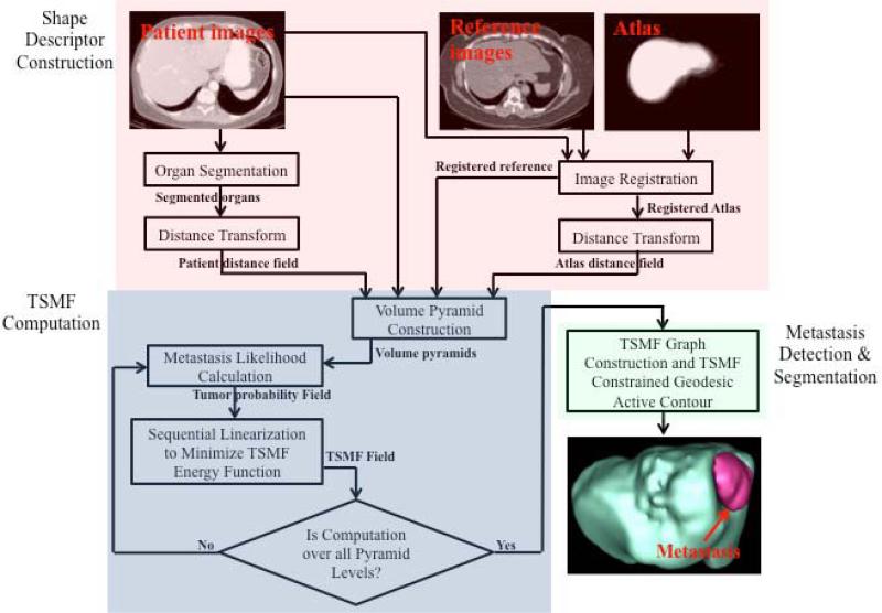
Fig. 3 summarizes our TSMF method for detection and segmentation of ovarian cancer metastases. It consists of three main steps: shape descriptor construction, TSMF computation, and metastasis detection and segmentation.
Figure 3.
Pipeline of tumor sensitive matching flow computation for detection and segmentation of ovarian cancer metastases. It consists of three main steps: shape descriptor construction (red rectangle), TSMF computation (blue), and metastasis detection and segmentation (green).
Shape descriptor construction aims to create two image pairs. One image pair consists of the patient image and a reference image, and the other pair is distance maps of the segmented organ and the probabilistic atlas. The first image pair contributes to find metastases in the image domain, and the second pair helps to identify them in the shape space. TSMF computation compares two image pairs within a variational framework and embeds a metastasis-likelihood function to yield the flow field only highlighted in the metastasis regions. Metastases can thus be identified by searching for large TSMF vectors. Moreover, the image regions containing large TSMF vectors approximately describe the metastasis shapes and they are used as the shape prior for metastasis segmentation, which effectively handles large variety of metastasis shapes. Ovarian cancer metastases (the red object in the bottom right image of Fig. 3) are finally segmented by integrating TSMF shape constraints into the geodesic active contour.
3.1. Shape Descriptor Construction
The purpose of this step is the creation of two image pairs. One pair describes the intensity difference between the patient image and a reference image, and the other is a pair of distance fields that encapsulate the shape differences between the patient organ and probabilistic atlas.
A CT image from a female patient without metastases is chosen as the reference image (top center image of Fig. 3). Interpatient organ difference was reduced by performing affine registration (Studholme et al., 1999) with 9-parameter affine transform on the reference image to globally match with the patient image. The registration accuracy was further improved by locally adjusting the reference image with a free-form deformation based on B-splines (Rueckert et al., 1999). Thus, both images are measured in the patient physical space, and comparing their intensity values becomes meaningful.
The construction of shape image pair consists of five main steps. 1) Liver and spleen are segmented using Linguraru's approach (Linguraru et al., 2010) because the objective of this work is the detection of perihepatic and perisplenic ovarian cancer metastases. This process initializes liver and spleen segmentation by aligning their atlases to the current patient image. The organ boundary is then refined using 4D-convolution and geodesic active contour, which leads to the final segmentation. 2) Distance transform (Maurer et al., 2003) is computed on liver and spleen segmentation to build organ distance fields. It is an iterative process that assigns the shortest distance to the nearest object boundary for every image point. Because the distance value can accurately measure the local shape variance as well as facilitate organ shape comparison in TSMF computation, distance field is chosen as the shape descriptor in our work. 3) Probabilistic liver and spleen atlases are established on the reference image. The top right image in Fig. 3 shows a probabilistic liver atlas constructed from ten liver segmentations. One liver segmentation is extracted from the reference image, and the remaining nine segmentations are registered to it by using affine registration (Studholme et al., 1999) with 9-parameter affine transform. The liver probabilistic atlas is measured in the reference image since all liver segmentations are converted into the reference image domain. The probabilistic liver atlas is finally established by averaging nine registered liver segmentation and the one from the reference image. A similar process is used to build spleen probabilistic atlas. Note that liver and spleen probabilistic atlases are created beforehand. Once it is established, it can be used to process different patient images. 4) Distance transform is computed on the probabilistic liver and spleen atlases. 5) We use the same registration process of the reference image and the patient image, to build shape image pairs for liver and spleen distance fields. Affine registration (Studholme et al., 1999) and non-rigid registration (Rueckert et al., 1999) are sequentially used to register the probabilistic atlas distance field to the organ distance field. Distance fields of the registered probabilistic atlas and the segmented organ are normalized to [0, 1], and comprise the final shape image pair.
3.2. TSMF Computation
The role of TSMF computation is to match shape and intensity image pairs within a variational framework. The key contribution of the TSMF computation is to embed a metastasis-likelihood function into the matching computation. TSMF vectors are thus magnified at the metastasis regions while suppressed in all other regions. Ovarian cancer metastases are detected by searching for large TSMF vectors.
Let Ip(p) and Ir(p) be the patient image and the reference image, and Dp(p) and Dr(p) be their corresponding distance fields (either liver or spleen shape image pairs), with u = (ux, uy, uz) be the TSMF vector at a point p = (x, y, z) in the image domain Ω. Assuming M(p) is the metastasis-likelihood function, the TSMF computation is formulated as a global energy function within a variational framework.
| (1) |
where , ε = 0.001 is a modified L1 norm and allows the computation to handle non-Gaussian deviations of the matching criterion (Brox et al., 2004; Papenberg et al., 2006). β = 50 and γ = 200 suggested by Brox (Brox, 2005) and α = 1000 experimentally determined in section 5.1.1 are constants to balance different components. Minimizing Eq. 1 generates TSMF vectors. Note that the weights of gradient constancy term and distance constancy term are dynamically controlled by M(p), which measures the possibility of metastasis existence in the local image region. The larger the value of M(p), the more likely the local region contains metastases. Distance and gradient terms with large M(p) will dominate the local TSMF computation. Therefore, TSMF vectors are enlarged at the locations where metastases are more likely to exist.
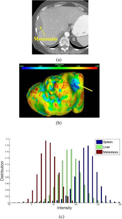
Next, we analyze the metastasis intensity and shape properties to define M(p). Fig. 4 illustrates a metastasis attached to the liver. We can see that the metastasis is darker than liver, and metastasis regions are also homogeneous (Fig. 4a). The intensity histograms of metastasis, liver, and spleen confirm this visual observation (Fig. 4c) because the metastasis intensities (red bars) are smaller than liver (green) and spleen (blue), and its intensity range is also narrow due to the homogeneity. Moreover, the metastasis intensity profile is similar to a Gaussian distribution. To account for individual variability, a Gaussian mixture model established on N representative metastases from different patients is used to describe the metastasis intensity distribution
| (2) |
where (μm)i and (σm)i are the mean intensity and standard deviation of i-th metastasis. N = 6 in this paper, which was experimentally determined in section 5.1.1.
Figure 4.
Metastasis intensity and shape properties for the definition of the metastasis-likelihood function. (a) A metastasis annotated by a yellow arrow, which is adjacent to the liver, (b) shape index distribution over the liver surface where blue to red means small to large values and the liver surface adjacent to the metastasis is also indicated by a yellow arrow, and (c) the intensity histograms of metastasis, liver, and spleen.
Metastases often push organs to deform and generate a cup shape on the organ surface (indicated by a yellow arrow in Fig. 4b). It is an important shape feature to discriminate the metastasis, and shape index (Koenderink and Doorn, 1992) is chosen to identify the cup shape. Letting 1 < 2 be the principal curvatures of the organ surface, the shape index at p is defined as
| (3) |
A cup shape has a small shape index value. We can find that the cup shape deformed by the metastasis is in blue, which corresponds to small shape index. Therefore, shape index can accurately identify the shape deformation caused by ovarian cancer metastases, though it also spots false positives when used alone.
M(p) is defined according to the Gaussian mixture model and shape index, which leads to Eqs. 4a-4c. Ωo and are the organ regions and non-organ regions in the patient image, and ∂ Ωo is the organ boundary. Dmax is the largest distance value in the patient distance field, and μ and σ are the mean intensity and standard deviation of an image region {q : |p − q| < 3 and }. This region contains a set of image points2q that are outside the organ and their distance to the current point p is less than 3 voxels, where the 3-voxel threshold is determined empirically. wi is the weight of i-th metastasis instance in Eq. 2 in terms of its population in the entire patient data. In this work, we set wi = 1. Note that M(p) is a piecewise function because we are only interested in detecting metastases near the organ surface. Eq. 4a indicates that the likelihood of the metastases existence remains a small value in the non-organ regions, and the likelihood is also penalized inside the organ in Eq. 4c because metastases inside organs are not our concern in this paper. Eq. 4b is designed to find metastases attached to the organ surface. The metastasis-caused shape variance is measured by |Dr(p) − Dp(p)|, which formulates the nominator. A large distance difference means high possibility of organ shape variance caused by metastasis existence. The denominator is composed of three components. The first two components measure the homogeneity and intensity difference between the current image region and the Gaussian mixture model of metastases. M(p) yields large values if the current mean intensity value stays within metastasis intensity ranges and the deviation also obeys the Gaussian mixture model. The shape index term is placed in the denominator since small values correspond to the cup shape caused by metastases. Thus, the response of Eq. 4b will be large if the current image region potentially contains metastases, and TSMF vectors will be enhanced. Otherwise, TSMF vectors will be suppressed.
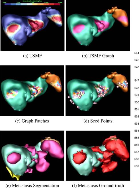
Calculus of variations is used to minimize Eq. 1 and estimate TSMF vectors. The numerical computation of calculus of variations is given in Appendix A. Fig. 5a shows the TSMF results mapped to the liver surface, where surface in red contains large TSMF vectors corresponding to the attached metastasis (Fig. 5f). Ovarian cancer metastases can thus be found by searching for large TSMF vectors.
Figure 5.
Process of ovarian cancer metastasis detection and segmentation. (a) TSMF results, (b) TSMF graph (pink) construction by connecting surface points with large TSMF vectors, (c) Graph patches (colored) by partitioning TSMF graph into many sub-graphs, (d) seed point (spheres), (e) metastasis segmentation by embedding seed points into TSMF-constrained GAC where yellow objects are false positives, and (f) Ground-truth metastases.
3.3. Metastasis Detection and Segmentation
Metastasis detection and segmentation consist of seed point determination and TSMF-constrained GAC (Fig. 5). Seed point determination constructs graphs on organ surface with large TSMF vectors and searches for a set of image points inside metastases. They are used as seed points for TSMF-constrained GAC to segment metastases. TSMF vectors also play the role of dynamical shape prior to constrain the GAC and to reduce inaccurate metastasis segmentation.
3.3.1. Seed Point Determination
The purpose of this step is to find a set of seed points inside metastases. Fig. 5 shows a patient with several perihepatic and perisplenic ovarian cancer metastases. The surface points with TSMF vector length larger than 10mm are first chosen and grouped into a TSMF graph, represented as red regions (Fig. 5b). Selected surface points form graph nodes and they are connected if they are adjacent on the organ surface. We set 10mm as the decision parameter because we are interested in detecting metastases larger than 10mm and TSMF vector length approximately represents the organ deformation caused by metastases.
Segmentation of large metastases requires the placement of multiple seed points to accurately represent
| (4a)(4b)(4c) |
the metastasis shape. For this reason, we partition the TSMF graph into sub-graphs with their areas approximately equal to 100mm2. Colored patches in Fig. 5c show the graph partition. Let Pi denote i-th patch and p = (x, y, z) be a point on Pi. Because u(p) measures the metastasis-caused shape variance at p and displacing p by u(p)/2 yields a new point inside the metastasis, the seed point q from Pi is computed as
| (5) |
Moreover, the intensity value of q should fall into the metastasis intensity range estimated in Eq. 2. Pink spheres in Fig. 5d represent the estimated seed points.
3.3.2. TSMF-Constrained Geodesic Active Contour
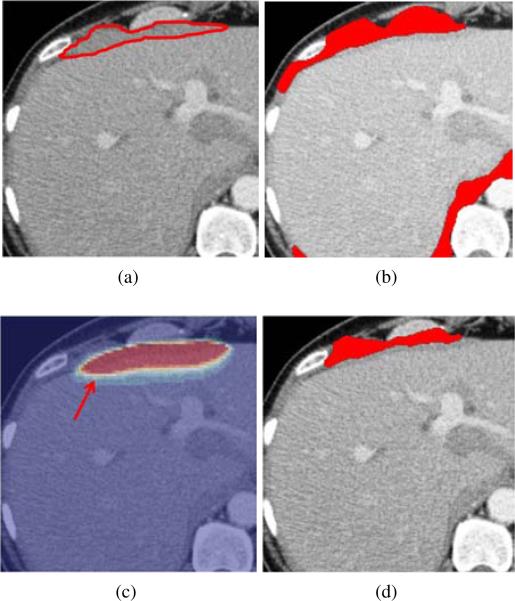
We embed seed points into our TSMF-constrained GAC to segment metastases. TSMF-constrained GAC augments conventional GAC (Caselles et al., 1997) based on the observation that image regions with large TSMF vectors approximately represent metastasis shapes (red regions in Fig. 6c). Therefore, TSMF can be used as shape constraints to prevent inaccurate metastasis segmentation (Fig. 6b) caused by weak edge response of metastasis boundaries. Moreover, TSMF constraints are dynamically established and adaptable to the current patient, which is a desirable property to handle a wide variety of metastasis shapes.
Figure 6.
TSMF shape constraints for metastasis segmentation. (a) A metastasis marked by red curves (ground truth); (b) inaccurate metastasis segmentation using conventional GAC; (c) Overlay of TSMF vectors on the original image, where image regions in red contain large TSMF vectors and regions in blue have small vectors; (d) metastasis segmentation using TSMF-constrained GAC (red regions in (c)).
We start with conventional GAC (Caselles et al., 1997) to derive the mathematical formulation of TSMF-constrained GAC. GAC is given by
| (6) |
where ϕ is a level set function, Ω is the image domain, G(x) = 1/(1 + x2), and the Heaviside function H is defined as
| (7) |
Conventional GAC forces ϕ to stop at image edges with large gradient magnitudes by minimizing Eq. 6.
TSMF shape constraints are represented as two addition terms that are embedded into Eq. 6. We include G(∇∥u(p)∥) to drive the level set function towards the boundaries of image regions with TSMF vector length larger than 10mm (red regions in Fig. 6c). Fig. 6c reveals that their boundaries are in the vicinity of the actual metastasis boundaries, such as a yellow curve pointed by a red arrow. Thus, level set propagation controlled by G(r[bardbl]u(p)[bardbl]) is also robust to the local gradients which are not the actual metastasis boundaries.
We also use a radial basis function to spatially relax the first TSMF shape constraint and adjust the level set to stop at the actual metastasis boundaries in the case that metastases are large.
| (8) |
Here, xi is an image point at the yellow curve and τ defines the width of relaxation regions. We set τ = 10, which is determined empirically based on the metastasis size in the validation dataset. Integrating two shape terms into Eq. 6 yields
| (9) |
Minimizing Eq. 9 with respect to ϕ generates the following gradient descent formulation.
| (10) |
To increase the convergence speed of level set propagation, we add a balloon model (Cohen, 1991) to Eq. 10 to prevent the level set from stopping on a nonsignificant local minimum. This term takes the propagation role, and Eq 10 is rewritten as
| (11) |
where λ is the weight of this propagation term. In this work, we experimentally set λ = 5. Fig. 6d shows the final metastasis segmentation by computing Eq. 11 and inaccurate metastasis segmentation is resolved thanks to the TSMF shape constraints.
4. Validation Datasets and Methods
We searched our Radiology Information System for CT scans of patients with known ovarian cancer during the period from 01/2008 to 12/2012 and obtained 239 records. We manually reviewed all CT images and found 57 women with ovarian cancer metastases. We then randomly chose an additional 57 women without metastases from the remaining 172 records. The validation datasets thus consisted of intravenous contrast-enhanced abdominal CT images from 114 women (age range, 17-81 years; mean age, 53±14 years). Retrospective analysis of these images was approved by our Institutional Review Board. CT images were generated with LightSpeed Ultra and QX/I [GE Health-care], Brilliance64 and iCT256 [Philips Healthcare], Definition and Biograph128 [Siemens Healthcare], and Aquilion ONE [Toshiba] scanners. The slice thickness ranged from 1mm to 5mm, and the in-slice resolution from 0.5mm to 0.98mm. 57 patients had at least one metastasis and the maximum number of metastases in one patient was fifteen. The total number of metastases was 226 (size range, 0.05-868.95cm3; mean size, 32.984cm3). 195 metastases were perihepatic and the remaining 31 were perisplenic. All metastases were manually segmented by two research fellows supervised by a board-certified radiologist and considered as the reference standard.
We explored two configurations of training and test datasets. One configuration was evenly and randomly to separate the validation dataset into the training dataset with 57 patient images (26 having at least one metastasis) and the test dataset with the other 57 patient images (31 having at least one metastasis). This configuration was only used for the comparison between the TSMF and OSP methods discussed in section 5.1.4 because the OSP method needs more training images to achieve high detection accuracy. The other configuration was to randomly choose six patient images with ovarian cancer metastases to compose the training dataset and define the metastasis-likelihood function for the TSMF. The remaining 108 patient images were used to formulate the test dataset. The choice of six patient images to form the training dataset is discussed in section 5.1.1.
A metastasis detection is considered to be a true positive if its segmentation overlaps that of the ground-truth by at least 20% of the volume of the ground truth. Otherwise, it is called false positive. To better understand metastasis detection using our TSMF algorithm, we experimentally evaluate two key parameters in Eq 1, the number of metastases to define the metastasis-likelihood function and the weight of the smoothness constraint term. The number of metastases used to define the metastasis-likelihood function is critical because a small number fails to describe metastasis appearance adequately while a large number requires that more training datasets be annotated, a time-consuming procedure. The weight of the smoothness term is important because small weights improve the sensitivity of metastasis detection but also increase the number of false positives, while large values can filter out false positives but decrease sensitivity. Determining optimized weights is thus important to balance the sensitivity and the number of false positives.
After these two parameters were determined through extensive experiments, we analyzed detection accuracy as a function of the metastasis size. We then compared the detection accuracy on perihepatic and perisplenic metastases. Finally, we compared TSMF with an organ surface partition (OSP) algorithm as the baseline method, which is similar to the sliding tangent circle algorithm (Bilello et al., 2004) to exhaustively find peripheral tumors on the liver surface. Peripheral liver tumors are similar to the ovarian cancer metastases because they are all growing near the liver boundaries. However, the tangent circle algorithm assumes that peripheral liver tumors are presented as spherical structures, and many other hepatic lesion detection methods (Joshi and Londhe, 2013; Bilello et al., 2004) also exploit this assumption. It is invalid in the detection of ovarian cancer metastases because ovarian cancer metastases present a wide variety of shapes (Figs. 1a and 1b). In addition, we want to point out that peripheral liver tumors are growing inside the liver while ovarian cancer metastases are transferred from other organs to the liver surface. Therefore, it is improper to directly compare TSMF with hepatic tumor detection algorithms
We study existing peripheral liver lesion detection algorithms (Hong et al., 2000; Bilello et al., 2004) that perform the greedy search of tumors on the organ surface, which leads to the organ surface partition (OSP) algorithm as the baseline approach. It decomposes the hepatic surface into 50 ~ 70 patches and the splenic surface into 15 ~ 25 patches (Fig. 7b). Instead of exploring the spherical shape and low intensity texture of hepatic tumors, OSP exploits the characteristic texture information of ovarian cancer metastases because their intensity values are constrained. The current surface patch is attached by a metastasis if the mean intensity value Ir of the adjacent image regions fulfilling (μm)i −(σm)i ≤ Ir ≤ (μm)i +(σm)i, where (μm)i and (σm)i are mean and standard deviation of i-th metastasis for defining Gaussian mixture model in Eq. 2. If the current surface patch satisfies the intensity condition, we create a set of metastasis features on this patch including shape index, average distance difference between the patient and reference images, mean and standard deviation of the intensity values of the adjacent image regions, local binary pattern (Ojala et al., 1996) and histogram of oriented gradients (Dalal and Triggs, 2005). Metastasis features are then imported into a SVM classifier trained on a dataset with 57 patient images. The classifier determines the final metastasis detections and removes false positives. Here, the SVM classifier uses Gaussian radial basis function as the kernel (Chang and Lin, 2011).
Figure 7.
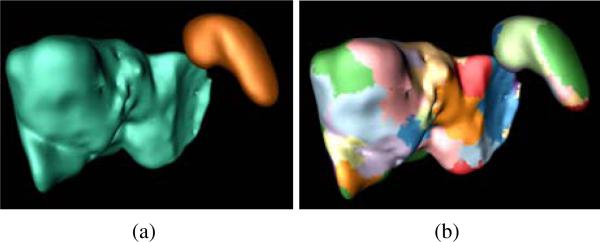
Organ surface partition method to detect ovarian cancer metastases and used as the baseline method to compare against TSMF. (a) Liver (cyan) and spleen (brown), (b) surface partition, where each colored component represents a partition.
The OSP algorithm preserves the main strategy of existing peripheral liver lesion detection algorithms (Hong et al., 2000; Bilello et al., 2004) that performs greedy search, and only modify the metastasis detection with the characteristic of metastasis intensity values. Thus, OSP is a reasonable baseline method to compare with TSMF.
We evaluated metastasis segmentation accuracy by only considering the segmentation of true positives. We compared the segmentation results of GAC and TSMF-constrained GAC to show the role of dynamical TSMF shape constraints in improving segmentation accuracy. Here, GAC also used seed points determined in section 3.3.1 to segment ovarian cancer metastases and was assigned with the same iteration number of level set propagation as the TSMF-constrained GAC. In our experiments, the segmentation accuracy was measured using six metrics defined in liver segmentation (Linguraru et al., 2010). They were volume overlap (VO), Dice coefficient (DC), relative absolute volume difference (RA), average symmetric absolute surface distance (ASD), symmetric RMS surface distance (RSD), and maximum symmetric absolute surface distance (MSD).
5. Experimental Results
In this section, we report the accuracy of metastasis detection and segmentation. All TSMF computations are carried out on a Windows machine with a six-core 2.67 GHz Intel Xeon CPU and 24 GB memory executing C/C++ code. The computational time on the detection and segmentation of perihepatic ovarian cancer metastases on high-resolution CT images (slice thickness less than 2mm) was 11 minutes, and it drops to 5 minutes on low-resolution CT images (5mm). The computational time on the perisplenic ovarian cancer metastases on high-resolution CT images was 6 minutes and it was 3 minutes on low-resolution CT images.
5.1. Detection Accuracy Evaluation
5.1.1. Key parameter selection
This section analyzed the choice of two key parameters in TSMF computation, including number of metastases to define the metastasis-likelihood function and weight of the smoothness constraint term in Eq. 1.
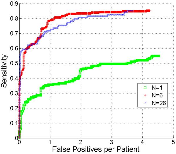
The free-response receiver operating characteristic (FROC) analysis (Hillis et al., 2009) was chosen to evaluate the metastasis detection accuracy. Fig. 8 compares the metastasis detection accuracy using 1, 6, and 26 metastases to define the metastasis-likelihood function. The comparison results indicate that at 2 false positives, the sensitivity of the metastasis function using six metastases (red curve) achieves 84% while it is only 44% (green) using one metastasis (p < 0.001 reported by JAFROC (Dorfman et al., 1992; Chakraborty, 2006)). However, the detection accuracies were comparable after we increased the number of metastasis from 6 to 26 (blue). This experiment confirmed that using six metastases to define the metastasis-likelihood function was sufficient to achieve high sensitivity while preserving a small number of false positives.
Figure 8.
Comparison of FROC curves of metastasis detection using 1, 6, and 26 metastases to define the metastasis-likelihood function.
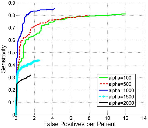
The weight α in the smoothness constraint term of Eq. 1 was evaluated in Fig. 9. Although setting α equal to 100 or 500 could increase the number of true positives compared with α larger than 1000, the number of false positives was also increased. Adjusting α to 1500 and 2000 reduced false positives with the side effect that actual metastases were also missed. Fig. 9 shows that 1000 is the optimum value for α yielding the highest sensitivity for a given number of false positives. Thus, we set α equal to 1000 in all our experiments.
Figure 9.
Comparison of FROC curves of metastasis detection by adjusting the weight α of smoothness constraint term in Eq. 1.
5.1.2. Perihepatic and perisplenic ovarian cancer metastasis detection
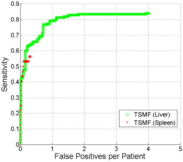
In this section, we compare the detection accuracy on perihepatic and perisplenic ovarian cancer metastases (Fig. 10). Because there were a small number of perisplenic ovarian cancer metastases and some patients had undergone splenectomy, the FROC curve for splenic metastases contains fewer points. The sensitivity of perihepatic metastasis detection was higher than perisplenic metastasis detection. The highest sensitivities for perihepatic and perisplenic metastasis detection were 86% and 57%, respectively. Both types of metastases had few false positives.
Figure 10.
Comparison of FROC curves of detection of perihepatic and perisplenic ovarian cancer metastasis.
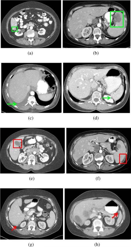
Typical examples of true positive, true negative, false positive, and false negative detections are shown in Fig. 11. Fig. 11a shows the true detection of a perihepatic metastasis even though its intensity values were similar to the liver parenchyma. The metastasis-likelihood function defined from six metastases identified the subtle intensity difference and successfully detected the lesion. TSMF also accurately distinguished fluid from metastases based on shape index although fluid and metastases can have similar intensity values (Fig. 11c). The gallbladder is the main source of false positives of perihepatic metastasis detection (Fig. 11e) because it has the same intensity levels and location as many metastases and can also produce the cup-shaped indentation on the liver surface. It accounts for 61% of the false positives in perihepatic metastasis detection. Other false positives are due to soft tissues at concave liver regions. Fig. 11g shows a difficult case in which intensity values of the metastasis were higher than normal and the metastasis was too small to deform the liver. Metastases less than 1cm3 accounted for 90% (15/17) of the false negatives. The 15 false negatives occurred in 9 patients.
Figure 11.
Typical examples of true positive (indicated by green rectangles), true negative (green arrows), false positive (red rectangles), and false negative (red arrows) on the detection of perihepatic ovarian metastases (left column) and perisplenic metastases (right column).
A true detection of perisplenic ovarian cancer metastasis is shown in Fig. 11b. In Fig. 11d, TSMF successfully excluded a kidney lesion that was similar to a metastasis and adjacent to the spleen. 90% of false positives in the detection of perisplenic ovarian cancer metastases were caused by muscles because they have similar intensity values to metastases and also surround part of the spleen (Fig. 11f). Fig. 11h depicts a false negative of a perisplenic metastasis because the spleen was inaccurately segmented and this metastasis was not attached to the spleen segmentation.
5.1.3. Metastasis volume influence
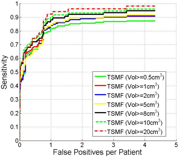
In the previous experiments, the detection accuracy was evaluated on all metastases regardless of volume. This section assesses the detection accuracy with respect to the metastasis volume because the volume is related to the clinical importance and detectability. In this experiment, the detection is not considered as false negative if the metastasis volume is less than a threshold. Fig. 12 shows FROC curves by thresholding metastasis volumes. Not surprisingly, at a rate of two false positives per patient, the sensitivity improved from 86% to 96% by increasing the threshold from 0.5cm3 to 20cm3. Note that the sensitivity was 90% when the threshold was 1cm3. In other words, our method was robust to detect metastasis larger than approximately 1 cm diameter.
Figure 12.
Comparison of FROC curves of metastasis detection with respect to metastasis volume.
5.1.4. Comparison of OSP and TSMF
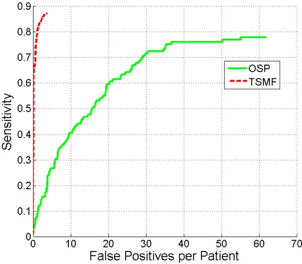
This section compares metastasis detection results of the TSMF and OSP methods. The total number of perihepatic and perisplenic metastases is 109 in the test dataset. For the TSMF method, there were 111 true detections (from 95 unique metastases) and 214 false positives. For the OSP method, there were 368 true postives (85 unique) and 3521 false positives. Fig. 13 shows the comparison results between TSMF and OSP on this test dataset. TSMF significantly outperforms OSP (p < 0.001 reported by JAFROC) because at 2 false positives, the sensitivity of OSP is less than 17% and TSMF is 87%.
Figure 13.
Comparison of FROC curves of metastasis detection using TSMF and OSP methods.
5.2. Evaluation of Segmentation Accuracy
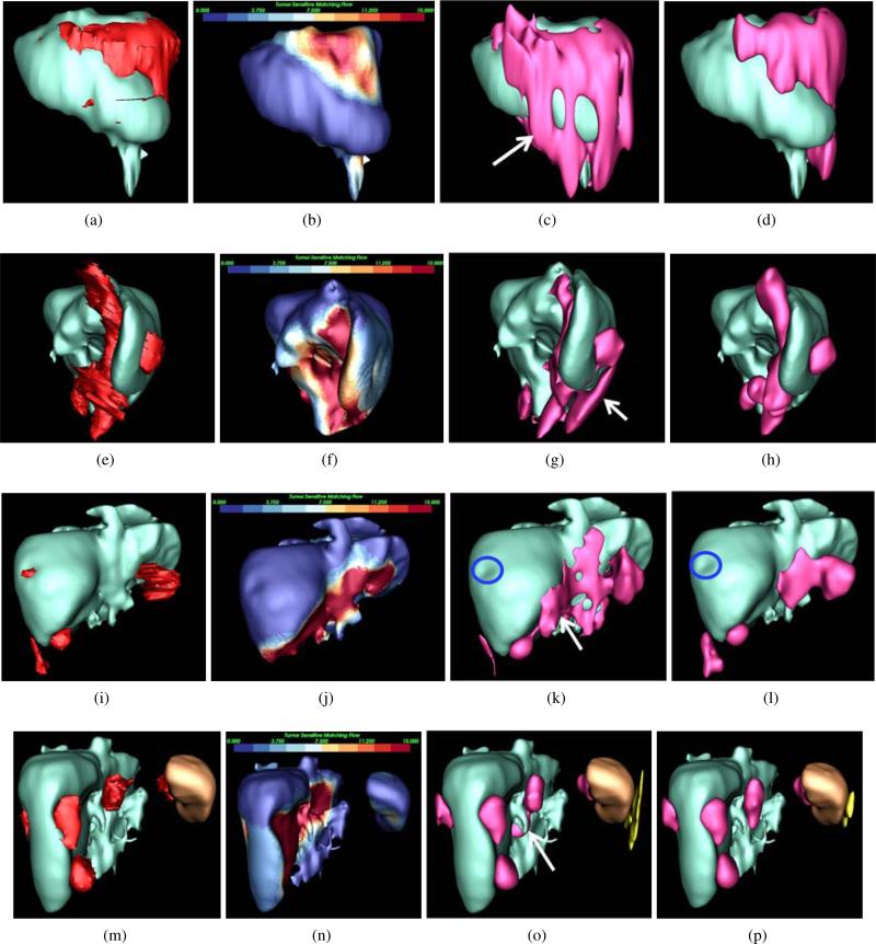
Table 1 shows the comparison results on metastasis segmentation using GAC and TSMF-constrained GAC. The TSMF-constrained GAC outperformed GAC on all six assessments (p < 0.001). Fig. 14 illustrates metastasis segmentation on four patients using GAC and TSMF-constrained GAC methods. From these four examples, we can find that TSMF-constrained GAC method can improve the metastasis segmentation over the conventional GAC because it exploits TSMF shape constraints in the level set propagation. It confirmed the findings in Table 1.
Table 1.
Comparison of segmentation accuracy using GAC and TSMF-constrained GAC. Wilcoxon signed rank test revealed that TSMF-constrained GAC significantly outperformed the conventional GAC based on six evaluation metrics (p < 0.001).
| Meth. | VO (%) | DC (%) | RA (%) | ASD (mm) | RSD (mm) | MSD (mm) |
|---|---|---|---|---|---|---|
| GAC | 42±26 | 58±29 | 25±13 | 7.0±6.0 | 10.2±6.9 | 39.6±13.9 |
| TSMF-GAC | 73±9 | 85±6 | 17±10 | 2.4±1.2 | 4.0±2.0 | 16.0±9.2 |
Figure 14.
Comparison of metastasis segmentation using GAC and TSMF-constrained GAC, where livers are visualized in cyan, metastases in red, spleen in brown and false positives in yellow. Metastasis ground-truths were given in the first column, and TSMF results were in the second column. Metastasis segmentations using GAC and TSMF-constrained GAC were shown in the third and fourth columns. Each row corresponds to a patient. The first patient at the top row was scanned with 5mm slice thickness. GAC caused metastasis over-segmentation (white arrow in (c)). Thanks to TSMF accurately detecting metastasis shapes in (b), the over-segmentation was relieved in (d). Metastasis clustering was observed in (e), and TSMF detected all these metastases. TSMF-constrained GAC also addressed over-segmentation (white arrow in (g)) generated by GAC. Although one metastasis less than 10mm in size (blue circles) was missed in the third patient, TSMF successfully detected all other metastases and TSMF-constrained GAC also reduced metastasis over-segmentation (white arrow in (k)). In the last patient, TSMF identified metastases adherent to both spleen and liver with one false positive on the spleen. TSMF-constrained GAC was again superior to GAC in dealing with over-segmentation (white arrow in (o)).
6. Discussion
We developed a tumor sensitive matching flow (TSMF) method to address the difficult challenges of detection and segmentation of perihepatic and perisplenic ovarian cancer metastases. In contrast to spherical hepatic tumors with low intensity values and inside the liver, ovarian cancer metastases often present a wide variety of shapes on the liver and spleen surfaces and have weak boundaries with these organs. The TSMF method embeds a metastasis-likelihood function into the image matching process within a variational framework to address these challenges. The metastasis-likelihood function forces TSMF vectors to be enlarged if the current image region possibly contains metastases. Otherwise, the function suppresses TSMF vectors. Randomly distributed ovarian cancer metastases can be detected by searching for large TSMF vectors. Moreover, image regions with large TSMF vectors approximately represent metastasis shapes. This is an important visual cue that deals with inaccurate segmentation due to weak metastasis boundaries and a wide variety of metastasis shapes.
There are two key parameters that control metastasis detection accuracy. One parameter is the number of metastases that formulates Gaussian mixture model in Eq. 2 to describe the metastasis appearance. An accurate Gaussian mixture model is critical to define the metastasis-likelihood function in Eqs. 4a-4c. A small number of metastases is insufficient to measure metastasis appearance precisely, while increasing the number demands more data annotation. Moreover, a large number of metastases might decrease the sensitivity, as observed in Fig. 8 because it adds rare metastases to introduce outliers. Our experiments revealed that six metastases are sufficient to define an accurate metastasis-likelihood function, which is a significant advantage over the conventional computer-aided diagnosis algorithms (Doi, 2007; Tateyama et al., 2011; Xu et al., 2011) since they require a lot of training samples. The other parameter is the weight of smoothness constraint term in Eq. 1. Small weights leverage the sensitivity of metastasis detection but increase the number of false positives, while large values can reduce false positives but decrease the sensitivity. Our extensive experiments indicated that 1000 was the optimal value to balance the sensitivity and the number of false positives.
We compared the detection accuracy of perihepatic and perisplenic ovarian cancer metastases using the estimated key parameters in TSMF computation. The detection accuracy of perisplenic metastases is lower than perihepatic metastases (Fig. 10) because of inaccurate spleen segmentation and small perisplenic metastases. They are too small to push the spleen to deform, and shape index fails to identify such subtle deformation. Similarly, TSMF method also missed small perihepatic metastases. Moreover, the number of false positives on persplenic metastasis detection is also smaller than the perihepatic metastasis detection because 13 patients have undergone splenectomy. Muscle is the primary false positive in the detection of perisplenic ovarian cancer metastases, and gallbladder often misleads TSMF in perhepatic metastasis detection because it has the similar intensity values to the metastases and also yields a cup shape on the liver surface.
We analyzed the volume influence on the metastasis detection accuracy (Fig. 12). Obviously, large metastases are more robustly detected in comparison with small ones because they yield large deformation on the organ surface and have the similar intensity distributions to the Gaussian mixture model in Eq. 2. TSMF computation also enforces the existence of metastases because the smoothness term in Eq. 1 propagates the likelihood of metastasis existence on the organ surface. Fig. 12 indicated that the TSMF method achieved 90% sensitivity with only 2 false positives for metastases larger than 1cm3, a clinically important size category.
We also compared the detection accuracy between TSMF and OSP methods. OSP method was developed from the existing peripheral liver perihepatic tumor detection algorithms (Hong et al., 2000; Joshi and Londhe, 2013; Bilello et al., 2004) that performed the greedy search of tumors on the organ surface, except that metastasis intensity features based on Gaussian mixture model in Eq. 2 were used to replace spherical shape and low intensity values of hepatic tumors to perform metastasis detection. TSMF markedly outperformed OSP because TSMF has many desirable properties in detecting ovarian cancer metastases. It juxtaposes the roles of image matching and metastasis classification according to the metastasis-likelihood function. The image matching process measures the shape variance between the current patient organs and atlases, and the metastasis-likelihood function evaluates if the current shape variance is caused by metastases. The effectiveness of this strategy is demonstrated by the method's sensitivity of 87% at a rate of two false positives per patient.
TSMF vectors are also an important cue to guide metastasis segmentation. Image regions with large TSMF vectors approximately represent metastasis shapes (Fig. 6c). In contrast to conventional shape priors (Chan, 2005; Cremers et al., 2006) that were created beforehand, our TSMF shape priors are established on the detection phase and are adaptable to an individual patient. Thus, the TSMF shape priors are an efficient means to guide segmentation of a wide variety of metastasis shapes. Embedding TSMF shape priors into a geodesic active contour significantly improves the accuracy of metastasis segmentation. The volume overlap rate of the TSMF-constrained geodesic active contour was markedly greater and the average surface distance markedly smaller than those from the conventional geodesic active contour. The detection accuracy of TSMF method is slightly better than existing hepatic tumor detection approaches (Hong et al., 2000; Joshi and Londhe, 2013; Bilello et al., 2004; Zhang et al., 2011) because their results were 87% sensitivity with 2.5 false positives per patient and TSMF also generated 87% sensitivity but with 2 false positives per patient. Moreover, comparing metastasis segmentation with hepatic tumor segmentation in the MICCAI challenge (Deng and Du, 2008), TSMF-constrained geodesic active contour yielded smaller relative absolute volume difference than the state-of-the-art hepatic tumor segmentation method (Stawiaski et al., 2008) (17% vs. 24%), and they have comparable average surface distance errors (2.4mm vs. 1.5mm). This result is encouraging considering that Stawiaski's approach is interactive while our approach is fully-automatic.
In the future, we will develop gallbladder atlas and embedding it into our detection framework to reduce false positives. We are also planning to detect and segment ovarian cancer metastases attached to other organs such as the colon and small bowel. Metastases elsewhere in the abdomen and not adjacent to organs are also being studied. Multi-organ segmentation (Linguraru et al., 2012a) is a potential approach to extend our TSMF method to these applications.
Another important issue is to distinguish fluid from perihepatic ovarian cancer metastases. In Fig. 11c, TSMF successfully excluded pleural fluid because the fluid was disconnected from the ovarian cancer metastases. In some challenging images, perihepatic fluid is present. Perihepatic fluids similar intensity values to some metastases may mislead TSMF to consider the fluid as a metastasis. Also, over-segmentation of actual metastases can occur if both fluid and metastases are present. Since perihepatic fluid tends to wrap around the liver and have large volumes, we are currently studying these two features to eliminate such fluid from our detection results.
The TSMF method missed some small metastases, and there is still room for improving metastasis segmentation accuracy. Joint detection and segmentation of ovarian cancer metastases (Liu et al., 2013) is a potential strategy to deal with this problem. In this strategy, accurate metastasis detection provides a precise TSMF shape prior for metastasis segmentation, and likewise accurate metastasis segmentation contributes to the metastasis detection.
7. Conclusions
We presented a variational framework to accurately detect and segment perihepatic and perisplenic ovarian cancer metastases by 1) juxtaposing the roles of metastasis classification / image matching to generate a tumor sensitive matching flow, 2) searching for image regions with large TSMF vectors to detect ovarian cancer metastases, and 3) embedding the detected image regions as the metastasis shape priors into the geodesic active contour to segment metastases. These beneficial properties lead our TSMF method to efficiently address the inherent challenges of metastasis detection and segmentation, including metastases randomly attaching to the liver or spleen, weak metastasis boundaries, and a wide variety of metastasis shapes. Validation on a large dataset demonstrated that TSMF can accurately detect perihepatic and perisplenic ovarian cancer metastases on contrast-enhanced CT images. The accurate detection and segmentation of ovarian cancer metastases have the potential to greatly impact clinical diagnosis and treatment on the women with ovarian cancer.
Highlights.
Detect and segment ovarian cancer metastases outside the liver and spleen.
Require a few patient images to formulate the training dataset.
Achieve higher detection accuracy than existing approaches.
Create dynamic shape priors to segment metastases with a wide variety of shapes.
Embed shape priors into the level set framework for metastasis segmentation.
Acknowledgements
This work was supported by the Intramural Research Program of the National Institutes of Health, Clinical Center. The authors thank Brandon Peplinski for data annotation.
Appendix A. Numerical Computation of Tumor Sensitive Matching Flow
To simplify the description, we first define some abbreviations.
| (A.1) |
The Euler-Lagrange equation of Eq. 1 corresponding to x-component is expressed as
| (A.2) |
Similar equations can be derived for the y and z components. We treat M(p) as a constant value in Eq. A.2 at each image point because 1) derivatives of the piecewise function M(p) are void at some image points; 2) M(p) is independent of u and its value is nearly constant at each iteration in resolving Eq. A.2; and 3) simplifying M(p) calculation significantly reduces the computational cost and complexity while preserving the accuracy of TSMF vectors. Our experimental results in section 5 also confirmed that such simplification is reasonable in TSMF computation. However, Eq. A.2 is still highly non-linear and non-convex. Two numerical strategies, multi-scale analysis and sequential linearization, are employed to resolve these two issues.
Multi-scale analysis is an efficient approach to handle the non-convexity of Eq. A.2 because the solution in the coarse scale can better approximate the global minimum. Three-level volume pyramids are constructed to create multi-scale space on patient and reference images as well as their distance fields. Sampling rate is 0.75 to ensure the smooth transition between different scales. Sequential linearization is another numerical strategy to remove non-linearity in Eq. A.2. It is represented as two nested fixed-point iterations. Assuming k is the pyramid level and l is the outer iteration index, Eq. A.2 is converted to Eq. A.3
However, Eq. A.3 still remains nonlinear because , , and are related to the estimated variables , , and . The inner iteration is thus introduced to decouple such correlation. Assuming m is the inner iteration index, we derive Eq. A.4 from Eq. A.3. We can observe that , , and are decoupled with , , and . Eq. A.4 is thus converted into a linear equation. We can derive the similar equations for the y and z components. Finally, we obtain a massive linear equation with three unknown TSMF vector components at each image point. Successive over-relaxation (Young, 1999) is used to solve this large linear system. After two nested iterations exceed predefined values at the current pyramid level, the solutions are used as the initialization for the next pyramid level through bilinear interpolation. TSMF field is generated after the computation is accomplished at the third, finest pyramid level.
| (A.3) |
| (A.4) |
Footnotes
Publisher's Disclaimer: This is a PDF file of an unedited manuscript that has been accepted for publication. As a service to our customers we are providing this early version of the manuscript. The manuscript will undergo copyediting, typesetting, and review of the resulting proof before it is published in its final citable form. Please note that during the production process errors may be discovered which could affect the content, and all legal disclaimers that apply to the journal pertain.
References
- Acar B, Napel S, Paik D, Cokturk B, Tomasi C, Beaulieu C. Using optical flow fields for polyp detection in virtual colonoscopy. Proceedings of the International conference on Medical Image Computing and Computer-Assisted Intervention. 2001:637–644. [Google Scholar]
- Bilello M, Gokturk S, Desser T, Napel S, Jeffrey RJ, Beaulieu C. Automatic detection and classification of hypodense hepatic lesions on contrast-enhanced venous-phase ct. Med. Phys. 2004;31:2584–2593. doi: 10.1118/1.1782674. [DOI] [PubMed] [Google Scholar]
- Black MJ, Jepson A. Estimating optical flow in segmented images using variable-order parametric models with local deformations. IEEE Transactions on Pattern Analysis and Machine Intelligence. 1996;18:972–986. [Google Scholar]
- Brox T. Ph.D. thesis. Saarland University; 2005. From pixels to regions: partial differential equations in image analysis. [Google Scholar]
- Brox T, Bruhn A, Papenberg N, Weickert J. High accuracy optical flow estimation based on a theory for warping. Proceedings of 8th European Conference on Computer Vision. 2004;4:25–36. [Google Scholar]
- Brox T, Rousson M, Deriche R, Weickert J. Colour, texture, and motion in level set based segmentation and tracking. Image and Vision Computing. 2010;28:376–390. [Google Scholar]
- Brox T, Weickert J. Level set segmentation with multiple regions. IEEE Transactions on Image Processing. 2006;15:3213–3218. doi: 10.1109/tip.2006.877481. [DOI] [PubMed] [Google Scholar]
- Cancer-Genome-Atlas-Research-Network Integrated genomic analyses of ovarian carcinoma. Nature. 2011;474:609–615. doi: 10.1038/nature10166. [DOI] [PMC free article] [PubMed] [Google Scholar]
- Caselles V, Kimmel R, Sapiro G. Geodesic active contours. Int J Comput Vision. 1997;22:61–79. [Google Scholar]
- Chakraborty D. Analysis of location specific observer performance data: validated extensions of the jackknife free-response (jafroc) method. Acad Radiol. 2006;13:1187–1193. doi: 10.1016/j.acra.2006.06.016. [DOI] [PubMed] [Google Scholar]
- Chan T. Level set based shape prior segmentation. Proceedings of the IEEE Conference on Computer Vision and Pattern Recognition. 2005:1164–1170. [Google Scholar]
- Chan T, Vese L. Active contours without edges. IEEE Transactions on Image Processing. 2001;10:266–277. doi: 10.1109/83.902291. [DOI] [PubMed] [Google Scholar]
- Chang C, Lin C. Libsvm: A library for support vector machines. ACM Transactions on Intelligent Systems and Technology. 2011;2:1–27. [Google Scholar]
- Chen F, Chung P, Chen C, Tsai H, Chang C. An automatic diagnostic system for ct liver image classification. IEEE Transactions on Biomedical Engineering. 1998;45:783–794. doi: 10.1109/10.678613. [DOI] [PubMed] [Google Scholar]
- Chen T, Zhang W, Good S, Zhou K, Comaniciu D. Automatic ovarian follicle quantification from 3d ultrasound data using global/local context with database guided segmentation. Proc. of International Conference on Computer Vision. 2009:795–802. [Google Scholar]
- Cohen L. On active contours models and ballons. Computer Vision, graphics and image processing. 1991;53:211–218. [Google Scholar]
- Cremers D, Rousson M, Deriche R. A review of statistical approaches to level set segmentation: Integrating color, texture, motion and shape. Int J Comput Vision. 2007;72:195–215. [Google Scholar]
- Cremers D, Sochen N, Schnorr C. Towards recognition-based variational segmentation using shape priors and dynamic labeling. Proceedings of the International conference on Scale Space. 2003:388–400. [Google Scholar]
- Cremers D, Sochen N, Schnorr C. A multiphase dynamic labeling model for variational recognition-driven image segmentation. Int J Comput Vision. 2006;66:67–81. [Google Scholar]
- Dalal N, Triggs B. Histograms of oriented gradients for human detection. Proc. of IEEE Conference on Computer Vision and Pattern Recognition. 2005:886–893. [Google Scholar]
- Dambreville S, Rathi Y, Tannenbaum A. A framework for image segmentation using shape models and kernel space shape priors. IEEE Transactions on Pattern Analysis and Machine Intelligence. 2008;30:1385–1399. doi: 10.1109/TPAMI.2007.70774. [DOI] [PMC free article] [PubMed] [Google Scholar]
- Dawood M, Buther F, Lang N, Jiang X, Schafers K. Respiratory motion correction in 3d pet/ct with advanced optical flow algorithms. IEEE Transactions on Medical Imaging. 2008;27:1164–1175. doi: 10.1109/TMI.2008.918321. [DOI] [PubMed] [Google Scholar]
- Deng X, Du G. Editorial: 3d segmentation in the clinic: A grand challenge ii liver tumor segmentation. MICCAI Workshop. 2008 [Google Scholar]
- Doi K. Computer-aided diagnosis in medical imaging: Historical review, current status, and future potential. Computerized Medical Imaging and Graphics. 2007;31:198–211. doi: 10.1016/j.compmedimag.2007.02.002. [DOI] [PMC free article] [PubMed] [Google Scholar]
- Dorfman D, Berbaum K, Metz C. Roc characteristic rating analysis: Generalization to the population of readers and patients with the jackknife method. Invest. Radiol. 1992;27:723–731. [PubMed] [Google Scholar]
- Fleet D, Weiss Y. Optical flow estimation. In: Paragios N, Y.C., Faugeras O, editors. Mathematical models for Computer Vision. The Handbook; 2005. pp. 239–257. [Google Scholar]
- Freiman M, Cooper O, Lischinski D, Joskowicz L. Liver tumors segmentation from cta images using voxels classification and affinity constraint propagation. International Journal of Computer Assisted Radiology and Surgery. 2011;6:247–255. doi: 10.1007/s11548-010-0497-5. [DOI] [PubMed] [Google Scholar]
- Hame Y, Pollari M. Semi-automatic liver tumor segmentation with hidden markov measure model and non-parametric distribution estimation. Medical Image Analysis. 2012;16:140–149. doi: 10.1016/j.media.2011.06.006. [DOI] [PubMed] [Google Scholar]
- Hillis S, Berbaum K, Metz C. Recent developments in the dorfman-berbaum-metz procedure for multireader roc study analysis. Acad Radiol. 2009;15:647–661. doi: 10.1016/j.acra.2007.12.015. [DOI] [PMC free article] [PubMed] [Google Scholar]
- Hong J, Kaneko T, Sekiguchi R, Park K. Computer-aided diagnostic system based on liver ct image. Proceedings of the IAPR Conference on Machine Vision Applications; Tokyo, Japan.. 2000. [Google Scholar]
- Horn B, Schunck B. Determining optical flow. Artificial Intelligence. 1981;17:185–203. [Google Scholar]
- Janowczyk A, Chandran S, Singh R, Sasaroli D, Coukos G, Feldman M, Madabhushi A. Hierarchical normalized cuts: unsupervised segmentation of vascular biomarkers from ovarian cancer tissue microarrays. Proceedings of International Conference on Medical Image Computing and Computer-Assisted Intervention. 2009:230–238. doi: 10.1007/978-3-642-04268-3_29. [DOI] [PubMed] [Google Scholar]
- Joshi D, Londhe N. Automatic liver tumour detection in abdominal ct images. International Journal of Computer Technology and Electronics Engineering. 2013;3:25–30. [Google Scholar]
- Keeling S, Ring W. Medical image registration and interpola tion by optical flow with maximal rigidity. Jounral of Mathematical Imaging and Vision. 2005;23:47–65. [Google Scholar]
- Kichenassamy S, Kumar A, Olver P, Tannenbaum A, Yezzi A. Conformal curvature flows: From phase transitions to active vision. Archive for Rational Mechanics and Analysis. 1996;134:275–301. [Google Scholar]
- Kim J, Fisher J, Yezzi A, Cetin M, Willsky A. A non-parametric statistical method for image segmentation using information theory and curve evolution. IEEE Transactions on Image Processing. 2005;14:1486–1502. doi: 10.1109/tip.2005.854442. [DOI] [PubMed] [Google Scholar]
- Koenderink J, Doorn A. Surface shape and curvature scales. Image and Vision Computing. 1992;10:557–564. [Google Scholar]
- Krivanek A, Sonka M. Ovarian ultrasound image analysis: follicle segmentation. IEEE transactions on medical imaging. 1998;17:935–944. doi: 10.1109/42.746626. [DOI] [PubMed] [Google Scholar]
- Lengyel E. Ovarian cancer development and metastasis. The American journal of pathology. 2010;177:1053–1064. doi: 10.2353/ajpath.2010.100105. [DOI] [PMC free article] [PubMed] [Google Scholar]
- Linguraru M, Pura J, Pamulapati V, Summers R. Statistical 4d graphs for multi-organ segmentation from multi-phase abdominal ct. Medical Image Analysis. 2012a;16:904–914. doi: 10.1016/j.media.2012.02.001. [DOI] [PMC free article] [PubMed] [Google Scholar]
- Linguraru M, Richbourg W, Liu J, Watt J, Pamulapati V, Wang S, Summers R. Tumor burden analysis on computed tomography by automated liver and tumor segmentation. IEEE Transactions on Medical Imaging. 2012b;31:1965–1976. doi: 10.1109/TMI.2012.2211887. [DOI] [PMC free article] [PubMed] [Google Scholar]
- Linguraru M, Sandberg J, Li Z, Shah F, Summers R. Automated segmentation and quantification of liver and spleen from ct images using normalized probabilistic atlases and enhancement estimation. Medical Physics. 2010;37:771–783. doi: 10.1118/1.3284530. [DOI] [PMC free article] [PubMed] [Google Scholar]
- Linguraru M, Vasilyev N, Marx G, Tworetzky W, Nido PD, Howe R. Fast block flow tracking of atrial septal defects in 4d echocardiography. Medical Image Analysis. 2008;12:397–412. doi: 10.1016/j.media.2007.12.005. [DOI] [PMC free article] [PubMed] [Google Scholar]
- Linguraru M, Yao J, Gautam R, Peterson P, Li Z, Linehan W, Summers R. Renal tumor quantification and classification in contrast-enhanced abdominal ct. Pattern Recognition. Special Issue on Cancer Detection. 1989;42:1149–1161. doi: 10.1016/j.patcog.2008.09.018. [DOI] [PMC free article] [PubMed] [Google Scholar]
- Liu J, Subramanian K, Yoo T, Uitert RV. A stable optic-flow method for tracking colonoscopy images. Proc. of Mathematical Methods in Biomedical Image Analysis (MMBIA) 2008:1–8. [Google Scholar]
- Liu J, Wang S, Linguraru M, Summers R. Tumor sensitive matching flow: An approach for ovarian cancer metastasis detection and segmenation. Proceedings of the MICCAI Workshop on Abdominal Imaging. 2012:265–273. [Google Scholar]
- Liu J, Wang S, Linguraru M, Yao J, Summers R. A variational framework for joint detection and segmentation of ovarian cancer metastases. Proc. of Medical Image Computing and Computer-Assisted Intervention. 2013 doi: 10.1007/978-3-642-40763-5_11. [DOI] [PMC free article] [PubMed] [Google Scholar]
- Lucas BD, Kanade T. An iterative image registration technique with an application to stereo vision. Proceedings of the International Joint Conference on Artificial Intelligence. 1981:281–288. [Google Scholar]
- Mala K, Sadasivam V, Alagappan S. Neural network based texture analysis of liver tumor from computed tomography images. International Journal of Biological and Life Sciences. 2006;2:33–40. [Google Scholar]
- Maurer C, Qi R, Raghavan V. A linear time algorithm for computing exact euclidean distance transforms of binary images in arbitrary dimensions. IEEE Transactions on Pattern Analysis and Machine Intelligence. 2003;25:265–270. [Google Scholar]
- Memarzadeh S, Berek J. Advances in the management of epithelial ovarian cancer. J Reprod Med. 2001;46:621–629. [PubMed] [Google Scholar]
- Moitz J, Bornemann L, Dicken V, Peitgen H. Segmentation of liver metastases in ct scans by adaptive thresholding and morphological processing. Proc. of MICCAI Workshop on 3D Segmentation in the Clinic: A Grand Challenges II. 2008 [Google Scholar]
- Mumford D, Shah J. Optimal approximations by piecewise smooth functions and associated variational problems. Communications on Pure and Applied Mathematics. 1989;42:577–685. [Google Scholar]
- NCI . Ovarian cancer. National Cancer Institute; 2013. http://www.cancer.gov/cancertopics/types/ovarian. [Google Scholar]
- Nougaret S, Addley H, Colombo P, Fujii S, Sharif SA, Tirumani S, Jardon K, Sala E, Reinhold C. Ovarian carcinomatosis: how the radiologist can help plan the surgical approach. Radiographics. 2012;32:1775–1800. doi: 10.1148/rg.326125511. [DOI] [PubMed] [Google Scholar]
- Ojala T, Pietikainen M, Harwood D. A comparative study of texture measures with classification based on feature distributions. Pattern Recognition. 1996;29:51–59. [Google Scholar]
- Papenberg N, Bruhn A, Brox T, Didas S, Weickert J. Highly accurate optic flow computation with theoretically justified warping. Intrernational Journal of Computer Vision. 2006;67:141–158. [Google Scholar]
- Paragios N, Deriche R. Geodesic active regions: A new framework to deal with frame partition problems in computer vision. Journal of Visual Communication and Image Representation. 2002;13:249–268. [Google Scholar]
- Prisacariu V, Reid I. Nonlinear shape manifolds as shape priors in level set segmentation and tracking. Proc. of IEEE Conference on Computer Vision and Pattern Recognition. 2011:223–247. [Google Scholar]
- Rueckert D, Sonoda L, Hayes C, Hill D, Leach M, Hawkes D. Non-rigid registration using free-form deformations: Application to breast mr images. IEEE Transactions on Medical Imaging. 1999;18:712–721. doi: 10.1109/42.796284. [DOI] [PubMed] [Google Scholar]
- Schmidt G, Binnig G, Kietzman M, Kim J. Cognition network technology for a fully automated 3d segmentation of liver tumors. Proceedings of the MICCAI Workshop on 3D Segmentation in the Clinic: A Grand Challenges II. 2008 [Google Scholar]
- Sean H, Bullitt E, Gerig G. Level set evolution with region competition: Automatic 3d segmentation of brain tumors. Proc. of International Conference on Pattern Recognition. 2002:532–535. [Google Scholar]
- Sethian J. Level set Methods: evolving interfaces in computation geometry, fluid mechanics, computer vision, and materials science. Cambridge University Press; 1999. [Google Scholar]
- Shimizu A, Narihira T, Furukawa D, Kobatake H, Nawano S, Shinozaki K. Ensemble segmentation using adaboost with application to liver lesion extraction from a ct volume. Proceedings of the MICCAI Workshop on 3D Segmentation in the Clinic: A Grand Challenges II. 2008 [Google Scholar]
- Signolle N, Plancoulaine B, Herlin P, Revenu M. Texture-based multscale segmentation: Application to stromal compartment characterization on ovarian carcinoma virtual slides. Proceedings of International conference on Image and Signal Processing. 2008:173–182. [Google Scholar]
- Singh A. An estimation-theoretic framework for image-flow computation. Proc. of International Conference on Computer Vision. 1990:168–177. [Google Scholar]
- Smeets D, Loeckx D, Stijnen B, Dobbelaer B, Vandermeulen D, Suetens P. Semi-automatic level set segmentation of liver tumors combining a spiral-scanning techniques with supervised fuzzy pixel classification. Medical Image Analysis. 2010;14:13–20. doi: 10.1016/j.media.2009.09.002. [DOI] [PubMed] [Google Scholar]
- Smeets D, Stijnen B, Loeckx D, Dobbelaer B, Suetens P. Segmentation of liver metastases using a level set method with spiral-scanning technique and supervised fuzzy pixel classification. Proceedings of the MICCAI Workshop on 3D Segmentation in the Clinic: A Grand Challenges II. 2008 [Google Scholar]
- Stawiaski J, Decenciere E, Bidault F. Interactive liver tumor segmentation using graph-cuts and watershed. Proceedings of the MICCAI Workshop on 3D Segmentation in the Clinic: A Grand Challenges II. 2008 [Google Scholar]
- Studholme C, Hill D, Hawkes D. An overlap invariant entropy measure of 3d medical image alignment. Pattern Recognition. 1999;32:71–86. [Google Scholar]
- Sundaram P, Zomorodian A, Beaulieu C, Napel S. Colon polyp detection using smoothed shape operators: preliminary results. Medical Image Analysis. 2007;12:99–119. doi: 10.1016/j.media.2007.08.001. [DOI] [PubMed] [Google Scholar]
- Tateyama T, Wei X, Zhou J, Wakamiya M, Kanasaki S, Furukawa A, Chen Y. Liver tumor detection in ct images by adaptive contrast enhancement and the em/mpm algorithm. Proceedings of the IEEE International Conference on Image Processing. 2011:1421–1424. [Google Scholar]
- Tuma R. Sometimes size does not matter: reevaluating recist and tumor response rate endpoints. Journal of the National Cancer Institute. 2006;98:1272–1274. doi: 10.1093/jnci/djj403. [DOI] [PubMed] [Google Scholar]
- Weickert J, Bruhn A, Brox T, Papenberg N. A survey on variational optical flow for small displacements. 2006 [Google Scholar]
- Wu D, Liu D, Suehling M, Zhou K, Tietjen C. A cascade learning method for liver lesion detection in ct images, in: Proc. of Medical Computer Vision. Recognition Techniques and Applications in Medical Imaging. Lecture Notes in Computer Science. 2013:206–214. [Google Scholar]
- Xu J, Suzuki K, Hori M, Oto A, Baron R. Proceedings of the SPIE Medical Imaging: Computer-Aided Diagnosis. Orlando, FL.: 2011. Computer-aided detection of hepatocellular carcinoma in multiphase contrast-enhanced hepatic ct: a preliminary study. [Google Scholar]
- Young D. Iterative Solution of Large Linear Systems (Computer Science and Applied Mathematics) 1 ed. Academic Press; 1999. [Google Scholar]
- Zhang S, Zhan Y, Dewan M, Huang J, Metaxas D. Towards robust and effective shape modeling: Sparse shape composition. medical image analysis. Medical Image Analysis. 2012;16:265–277. doi: 10.1016/j.media.2011.08.004. [DOI] [PubMed] [Google Scholar]
- Zhang X, Furukawa T, Zhou X, Hara T, Kanematsu M, Fujita H. Proceedings of the SPIE Medical Imaging: Computer-Aided Diagnosis. Orlando, FL.: 2011. Detection of metastatic liver tumor in multi-phase ct images by using a spherical gray-level differentiation searching filter. [Google Scholar]
- Zhou J, Xiong W, Tian Q, Qi Y, Liu J, Leow W, Han T, Venkatesh S, Wang S. Semi-automatic segmentation of 3d liver tumors from ct scans using voxel classification and propagational learning. Proceedings of the MICCAI Workshop on 3D Segmentation in the Clinic: A Grand Challenges II. 2008 [Google Scholar]
- Zhu SC, Yuille A. Region competition: Unifying snakes, region growing, and bayes/mdl for multi-band image segmentation. IEEE Transactions on Pattern Analysis and Machine Intelligence. 1996;18:884–900. [Google Scholar]
- Zimmer H, Bruhn A, Weickert J. Optic flow in harmony. Intrernational Journal of Computer Vision. 2011;93:368–388. [Google Scholar]


