Measuring the Level and Inequality of Wealth: An Application to China

Abstract

We construct and compare three distinct measures of household asset wealth that complement traditional income- or expenditure-based measures of socioeconomic status. We apply these measures to longitudinal household survey data from China and demonstrate that household asset wealth has been increasing over time, a theme consistent with many previous studies on the process of development in China. Unlike other studies that have shown rising income inequality over time, however, we show that asset wealth inequality has actually been declining in recent years, indicating widespread participation in the benefits of economic reforms. Furthermore, the evolution in the cumulative distribution of household welfare is such that social welfare has been increasing with the passage of time, despite rising inequality in the early years of the survey.

1 Introduction

One of the primary objectives of development policy is to increase the living standards of individuals in developing countries (Deaton, 1997). In order to evaluate the effects of various policies on the level and distribution of welfare within or across particular populations, researchers must find an appropriate method or measurement with which to make comparisons. The traditional measures by which researchers have assessed living standards are income- or expenditure-based measures, typically computed from household budget and consumption surveys. These measures are advantageous since they have primitive monetary interpretations and can easily be used to assess the impacts of various policies on social outcomes such as poverty and inequality. Despite their popularity, however, these measures can be problematic for a number of different reasons, particularly in developing countries. For starters, there can be rather wide divergences between income and consumption. Incomes, particularly in developing countries, can exhibit discrete lumpiness and have a great deal of seasonal variation, whereas consumption expenditures are generally much smoother, consistent with predictions of the permanent income hypothesis (Friedman, 1957). The smoothness in consumption is facilitated by credit markets, through which households can save current income to finance future consumption or, contrarily, borrow from future income to finance current consumption. There are also challenges associated with accurately measuring full income or expenditures. Reported household incomes generally include only wages or market income, while full household income often also consists of like-kind earnings as well as the value of home production and leisure time. Similarly, reported consumption expenditures generally only capture market transactions, and therefore ignore the value of non-market transactions and the consumption of home-produced goods and services. Additionally, data on household income may be problematic due to systematic biases in reported incomes–as well as systematic non-responses. Consumption expenditures are generally less susceptible to these potential biases, but basing a measure of well-being on current expenditures fails to consider that many goods that households purchase have usable lives beyond just the current period. Expenditure-based measures may therefore only capture a short-term snapshot of a household’s true well-being. There is also the non-trivial issue that spatial and temporal price differences require making potentially complex adjustments to expenditure figures in order to facilitate comparisons (Deaton and Zaidi, 2002).

There are additional components of welfare which are excluded from traditional measures because they cannot easily be assigned a monetary value (Deaton and Zaidi, 2002). Sen (1999) argued that money or income should not be valued in and of itself, since it is merely a means to an end, namely the freedom “to lead the kind of lives [we] value–and have reason to value” (p. 18). A measure of welfare consistent with this view would incorporate other dimensions than simply monetary dimensions, and would embody a household’s broad set of capabilities. It is extremely difficult (if not impossible) to actually measure a household’s capabilities; capabilities are not measured based on the results actually achieved, but the achieved results are often indicative of the underlying capabilities. In practice, it is much more feasible to focus on a household’s assets, which are indicators of a household’s capabilities, and therefore its multidimensional welfare. Measures that capture a household’s command over assets and other forms of capital would presumably be more representative of the underlying achievement of a household, or what they manage to do or be (Sahn and Stifel, 2003), since the underlying functionings of the assets are indicative of the household’s capabilities or freedoms (see Sen, 1987), and may therefore provide a more holistic picture of a household’s well-being and allow for a richer analysis on policy impacts.

In this paper we examine three measures of household asset wealth that characterize these dimensions of welfare. Since these measures ignore financial capital, they can most appropriately be viewed as complements to traditional measures. The three proposed measures differ in their measurement of household socioeconomic status. The first measure is most similar to traditional income- or expenditure-based measures, since it is based on subjective valuation of household capital and is a direct measure easily interpretable a measure of household monetary wealth. The remaining two measures are indices which, while not providing absolute measures, allow for relative comparisons. As with any index, the method of weighting index components is of critical importance. We consider three weighting strategies. We first follow a very simple approach, allowing the various factors to be weighed equally. We then consider an alternative factor weighting strategy based on the first principal components of the polyserial factor correlation matrix. Using longitudinal data from China, we construct these three measures and use them as the basis for an exploratory analysis regarding the effects of China’s economic reforms on welfare outcomes. The exploratory analysis generally suggests that asset wealth has been increasing over time in China, consistent with results based on income- and expenditure-based measures which have shown remarkable progress in poverty alleviation in China. The expansion of asset wealth illustrates an expansion of capabilities, especially as it pertains to basic levels of economic empowerment. However, while income- and expenditure-based measures have also tended to show uneven progress against poverty, with increasing income inequality suggesting that the benefits of reform policies have not been evenly distributed, we find evidence that the distribution of assets and other forms of capital (e.g., housing infrastructure) have become more egalitarian, with inequality declining since 2000 despite increases in inequality throughout most of the 1990s. If we consider an asset wealth measure as complementary to an income- or expenditure-based measure, these results may suggest that the total degree of inequality in China may be less severe than what would be suggested based solely on the results of income and expenditure surveys.

2 Proxy Measures of Household Well-Being

In recent years, measures based on household asset ownership and other forms of household capital have widely been used for comparisons of economic well-being. A pioneering application was Filmer and Pritchett (1998), who constructed an asset index to use as a proxy for socioeconomic status in predicting educational enrollment across states of India. Though initially motivated to find a proxy for household wealth in the absence of traditional income or expenditure data, their results suggest using an asset index is at least as reliable as using the more conventional measures. The use of these proxies has been widely adopted and applied for myriad purposes, many involving the analysis of the effects of socioeconomic status on various health and education outcomes: Bollen et al. (2001) use an asset index to predict fertility in Ghana and Peru; Filmer (2005) uses one to explain the frequency and treatment of fevers (potentially due to malaria) among children in twenty-two countries in sub-Saharan Africa; Sahn and Stifel (2003) use a wealth index to predict child nutrition indicators (e.g., stunting prevalence, height-for-age Z-scores); Sastry (2004) and Fay et al. (2005) use asset indices to explain various dimensions of child health and mortality; Case et al. (2004) and Ainsworth and Filmer (2006) use household wealth to examine educational enrollment in sub-Saharan Africa. Other researchers have used an asset index to perform exploratory analysis on the level, distribution, and dynamics of household wealth: Sahn and Stifel (2000) use an asset index as the measure with which to analyze poverty; McKenzie (2005) constructs a measure of inequality based on an asset index; Moser and Felton (2007) analyzes asset accumulation over time based on a series of asset indices. Many of these applications (including Filmer and Pritchett, 1998, Filmer, 2005, Fay et al., 2005, Case et al., 2004, Ainsworth and Filmer, 2006, Sahn and Stifel, 2000) have used Demographic and Health Survey (DHS) data, which lack data on consumption expenditures. A benefit of the construction of an asset index is that it is able to summarize a great deal of information in a single measure. In addition, an index circumvents some of the measurement error, non-response and recall biases, as well as other problems commonly associated with using standard measures: because household survey questions on asset ownership or forms of capital generally take the form of discrete indicators (typically either binary ownership indicators or ordinal, categorical indicators), these data are generally believed to be more reliable.¹ Household assets and other forms of capital are typically durable in nature, and may therefore provide a better picture of long-term standards of living than simply income or expenditures (Moser and Felton, 2007). Additionally, for credit constrained households, holding household wealth in the form of assets is an important means for de-coupling household income from household consumption, therefore maintaining the appeal of a smooth measure of well-being.

The first measure, based on subjective valuation of household capital, is a direct measure, easily interpreted as an absolute measure of monetary wealth. The remaining two measures are indices, based on indicators of household capital holdings. While these are not interpretable as direct or absolute measures of well-being, they do allow for easy interpretation as a relative measure of well-being (within their own class), and easily facilitate relative comparisons. As with any index, the choice of component weights (or factor loadings) is of critical importance. Following Moser and Felton (2007), we consider equal factor weights and factor weights determined based on the first principal components of the underlying factor correlation matrix.

2.1 Subjective Capital Valuation

A direct way of measuring household well-being is to sum the value of all household capital holdings. This measure of household well-being could be represented as

$$W_{1,\mathit{it}}^{\ast }={\displaystyle \sum }_{j=1}^J{p}_{\mathit{jt}}{x}_{\mathit{ijt}}$$ (1)

where p_jt is the price of asset j in period t and x_ijt is household i’s holding of asset j in period t. This measure of household wealth can be problematic, since price data can be difficult to obtain, especially in developing countries where many transactions are based on barter systems (Moser and Felton, 2007). A related measure sums the value of each of a household’s capital holdings, where the values are subjective responses given by survey respondents. This reformulated measure can be represented as

$$W_{1,\mathit{it}}={\displaystyle \sum }_{j=1}^J{v}_{\mathit{ijt}}$$ (2)

where, now, v_ijt is the value of household i’s holding of asset j during period t. This measure introduces problems of its own, since these valuations are completely subjective and are prone to (potentially significant) measurement error, which would then bias the measurement of welfare. If we decompose the household’s subjective valuation into a per-unit price (measured with error) and its asset ownership (which we assume the household measures without error), this measure could be written as

$$W_{1,\mathit{it}}={\displaystyle \sum }_{j=1}^J(p_{\mathit{jt}}+{\epsilon }_{\mathit{jt}})x_{\mathit{ijt}}={\displaystyle \sum }_{j=1}^J{p}_{\mathit{jt}}{x}_{\mathit{ijt}}+{\displaystyle \sum }_{j=1}^J{\epsilon }_{\mathit{jt}}{x}_{\mathit{ijt}}=W_{1,\mathit{it}}^{\ast }+{\displaystyle \sum }_{j=1}^J{\epsilon }_{\mathit{jt}}{x}_{\mathit{ijt}}.$$ (3)

We can easily see that allowing for subjective valuations biases our measure of household wealth. This bias is increasing with the measurement error associated with the household’s subjective per-unit price estimate. In addition to this bias, measuring well-being in this fashion ignores potentially important components of a household’s overall welfare. Such non-pecuniary dimensions may be difficult–if not impossible–to value (e.g., robust housing infrastructure, access to clean water and proper sanitation, etc.). Such capital may reflect socioeconomic status without necessarily serving a productive purpose nor storing value. Nevertheless, since this measure affords us a subjective measure of household well-being, which is often not available to researchers analyzing standard household income and expenditure surveys, we will consider this subjective valuation defined by equation (2) as a measure of well-being for comparison with our other measures.

2.2 Wealth Index: Equal-Weighted Asset and Capital Ownership

In using capital ownership indicators to construct an index to serve as a proxy for household well-being, equal component weights have the appeal of simplicity and relieve the researcher of the somewhat daunting task of assigning component weights. In addition, a wealth index allows for the inclusion of non-pecuniary dimensions of well-being that are excluded from direct, monetary measurements. For example, ordinal or categorical measures indicating the robustness of household infrastructure can easily be included. A measure of well-being using equal weights on household capital can be written as:

$$W_{2,\mathit{it}}={\displaystyle \sum }_{j=1}^J{x}_{\mathit{ijt}}$$ (4)

where, as before, x_ijt is household i’s holding of capital form j in period t. The capital indicator x_ijt is generally a discrete measure. It can be a count, a binary ownership indicator or capture ordinal rankings, as in the case of housing capital. A household with a concrete roof (score of 5) would be “wealthier” than a household with a huijiao (charcoal ash mixed with grey earth and mud) roof (score of 1). It should be readily apparent that W_2,it is simply a special case of $W_{1,\mathit{it}}^{\ast }$, where p_jt = 1 ∀j, t. That is, an equal-weighted index implicitly assumes the “value” (or contribution to well-being) of each form of capital is equal, and moreover equal to 1.

2.3 Wealth Index: Weightings Derived From Polyserial Principal Component Analysis

The final wealth measure we consider is a wealth index in which the weights are derived from principal component analysis (PCA). In our analysis, we create our index using only the first principal component. This choice is made for two reasons. First, by definition, the first principal component captures the greatest amount of information regarding the underlying latent variable. Second, the first principal component allows for an easy interpretation that is not necessarily available for higher order principal components. The first principal component can be interpreted as the “size” of the underlying latent variable being explained. In this case, the first principal component provides a measure of the “size” of a household’s welfare. Higher-order principal components provide information about the contributions of the index factors to characteristics of well-being that are orthogonal to the “size” of well-being, such as its structure.² Interpreting higher-order principal components in terms of the structure of wealth is neither straightforward nor necessarily an important aspect of this type of analysis. Our second maintains the discrete nature of the capital ownership indicators native to the data and employs polyserial PCA methods to generate the factor loadings (see Kolenikov and Angeles, 2009).

Standard PCA assumes that the components underlying the latent variable are distributed multivariate normal. If one normalizes the components, as is usually done for standard PCA, then such distributional assumptions may generally be satisfied, at least to an approximation. Normalization, however, imposes restrictions on how the factor weights can be interpreted: they must be interpreted as the contribution of a one standard deviation change in the ownership of the factor. If one desires to maintain the discrete nature of the underlying capital ownership indicators, and to compute scoring factors for each discrete measure, then standard methods are unsatisfactory. For example, if we have a binary ownership indicator, where the indicator is equal to one if the household owns the asset in question and zero otherwise, we may desire for our indexing method to compute scoring factors for both owning and not owning the asset. Moser and Felton (2007) note that, in some instances, not owning an asset may convey more information about household well-being than owning it. This is especially true if a substantial majority of the sample population owns a particular asset; the minority who do not own it should generally be regarded as particularly destitute. Kolenikov and Angeles (2009) propose the construction of wealth indices using PCA techniques on correlation matrices that maintain the discrete nature of the component data. These methods date back to Pearson (1900), who introduced tetrachoric correlations among binary variables using a two-by-two contingency table. This method was later expanded to polychoric correlations between non-binary discrete variables, such as counts or orderings (Pearson and Pearson, 1922), and later to polyserial correlations, which examines the relationship between discrete and continuous data. Polychoric and polyserial correlations differ from correlation coefficients for continuous variables and can be conceptualized as the “maximum likelihood estimates of the correlation between the unobserved normally distributed continuous variables underlying their discretized versions” (Kolenikov and Angeles, 2009, p. 135).

Generating our wealth measure from this procedure requires some additional notation. Consider an asset category j that takes discrete values $k={\underset{¯}{k}}_j,\mathrm{...},{\overline{k}}_j$. For a binary asset ownership indicator, for example, k = {0,1}; for an ordered variable such as a categorical variable, we might have k = {1, …, 4}. The estimated thresholds can be used to elicit coefficient scores for each unique level of the discrete asset variable:

$${\alpha }_{\mathit{jk}}=\frac{\exp \{-\frac{1}{2}{({\widehat{\tau }}_{j,k-1})}^2\}-\exp \{-\frac{1}{2}{({\widehat{\tau }}_{\mathit{jk}})}^2\}}{\sqrt{2\pi }[{\mathrm{\Phi }}_1({\widehat{\tau }}_{\mathit{jk}})-{\mathrm{\Phi }}_1({\widehat{\tau }}_{j,k-1})]}[{\mathrm{\lambda }}_j]$$ (5)

where α_jk is the coefficient score (or factor loading) associated with the k^th category of the j^th asset, λ_j is the first principal component associated with the j asset, and ${\widehat{\tau }}_{\mathit{jk}}$ are estimated thresholds derived from the marginal distributions of the observed discretized variables x_j (see Olsson, 1979). The α_kj term has the appealing feature that it allows for different factor loadings for different discrete values of ordinal, count, or binary data. In this case, the factor weight differential between two consecutive units of ownership (i.e., the difference in factor weights between owning, say, one unit and two units of a particular asset) would not be constant. This is captured by the additional subscript k in α_kj, which signifies that, in general, ${\alpha }_{{\underset{¯}{k}}_{j}j}\ne {\alpha }_{1_j}\ne \dots \ne {\alpha }_{{\overline{k}}_{j}j}$. It should be noted that, by construction, the factor weights are monotonic within asset classes and, since they are derived partially on the basis of the marginal distributions, they take into consideration the sample ownership of the different assets. We can then write a wealth index as:

$$W_{3,\mathit{it}}={\displaystyle \sum }_{j=1}^J{\displaystyle \sum }_{k={\underset{¯}{k}}_j}^{{\overline{k}}_j}{\alpha }_{\mathit{jk}}I(x_{\mathit{ijkt}})$$ (6)

where I(x_ijkt) is an indicator function for household i’s ownership of category k of asset j during time t. Returning to our binary asset example, suppose household i owns asset j during period t. Then I(x_ij0t) = 0 and I (x_ij1t) = 1. For the categorical asset, suppose household i owns category 3 of asset j during t. Then I(x_ij1t) = I(x_ij2t) = I(x_ij4t) = 0, and I(x_ij3t) = 1. Having different factor weights for different quantities or categories of ownership allows that the difference between α_j0 and α_j1 will not necessarily be the same as the difference between the scores for α_j1 and α_j2, even though the incremental increase in the asset ownership indicators is the same. This allows for richer analysis and comparisons that may more accurately reflect the relative wealth or deprivation of households based on their asset ownership-or lack thereof.

Note that, while capital holdings vary over time, the factor loadings are time-invariant, since the analysis is performed on the pooled data. Since the data span a rather long period of time, it is possible that the value of the different forms of capital have changed over time. In other words, it is possible that the contribution of a particular asset to household welfare may not be constant. Moser and Felton (2007) identified this issue and considered two alternate solutions. First, the analysis can be conducted separately for each survey year. While this approach allows us to see how the relative contributions of various assets change over time, it only facilitates inter-household comparisons of wealth within a particular survey year. Second, the data can be pooled over time and a single factor loading for each component can be computed using the aggregated data. By aggregating the data over time, one is able to make comparisons both within and across time periods. This is the approach Moser and Felton (2007) follow, and is likewise supported by McKenzie (2005) for making intertemporal comparisons. A similar argument could be made for aggregating data over other dimensions, such as spatial or urban/rural: using the same factor loadings across these other dimensions is the only way by which inter household comparisons can be made. This is supported by McKenzie (2005), who suggests pooling data on a geographic basis to facilitate inequality comparisons across geographic space. Since we are ultimately concerned with the ability to make inter-household and inter-temporal comparisons, pooling the data is a much more appealing option than performing the analysis using separate cross-sections.³

3 Data

The data used in this analysis come from the China Health and Nutrition Survey (CHNS), a longitudinal household survey conducted by the Carolina Population Center (CPC) at the University of North Carolina (UNC) and the National Institute of Food Safety at the Chinese Center for Disease Control and Prevention. Surveys were collected in 1989, 1991, 1993, 1997, 2000, 2004, and 2006, covering approximately 4,400 households. The CHNS data cover nine provinces in China, mostly in Eastern or East-Central China.⁴ A multistage, random cluster process was used to draw the samples in each province. Within each province, counties were stratified by income (low, medium, and high) and a weighted sampling scheme was used to select four counties in each province. While the survey is not nationally-representative, the selected communities and survey participants demonstrate a great deal of variation on many important socioeconomic characteristics.

Many household surveys in developing countries do not directly address household wealth. Rather, they typically only include information on asset ownership, often taking the form of binary or ordinal asset ownership indicators. These ordinal indicators typically consist of a series of ordered categories, with respondents indicating the category that captures their particular circumstances. Consistent with other surveys, the CHNS contains binary information on asset ownership for a broad variety of asset types, as well as ordinal rankings for such indicators as housing infrastructure, water sources, light sources, cooking fuels, and toilet facilities. For many assets, the surveys ask respondents regarding the quantity of these assets (or counts) owned. In addition, the CHNS is rather unique in that there are direct questions regarding the estimated value of many of these assets. This allows the computation of a measure of household wealth that has a strictly monetary interpretation.

We focus on 33 forms of capital that have consistent coverage across all survey waves. These can be decomposed into three broad categories: housing capital, physical non-productive capital (including both transportation goods and other household durables), and physical productive capital (including agricultural capital and non-agricultural commercial capital). These organization of these assets is illustrated in Figure 1. These can be considered as indicative of underlying capabilities because they either directly constitute improvements in livelihoods or because they indirectly represent such livelihood improvements insofar as they demonstrate the increased ability to substitute leisure for labor. Since it is both theoretically and operationally advantageous to have positive correlations between the indicators and the underlying variable being explained (i.e., wealth or welfare), we have re-ordered some of the categorical data such that increasing measures indicate increasing socioeconomic status. Tables A.1–A.3 in the online appendix report the forms of capital that fall under each of the three broad classifications, as well as their associated sample summary statistics. ⁵

Figure 1.

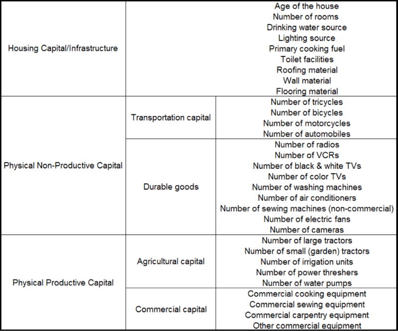
Assets and Other Forms of Capital Included in Wealth Indices

China presents an interesting context for which to analyze patterns in household welfare and inequality, particularly in light of the dramatic economic reforms that the Chinese government has initiated in an attempt to liberalize production and increase economic incentives. Reforms began in the agricultural sector in late 1978, during a time in which food supplies and agricultural production were deemed severely deficient. Initial reforms gave individual households more autonomy over land, labor and production decisions. In response to these reforms, grain output was nearly 33 percent higher in 1984 than it was in 1978 (Lin et al., 2003). The success of the reforms to rural organization gave reformers the confidence they needed to expand their reforms to other sectors. Chinese economic reforms have been very different than reforms undertaken by most other transitional economies. One of the key features of Chinese reforms is that they have generally been implemented on a very gradual basis, in stark contrast to the shock therapy approach that has been applied in other settings. The gradual nature of the economic reforms has been likened to “crossing the river by groping for stones”, implying the tentativeness and deliberateness with which reforms have been undertaken. Reforms have focused on maintaining stability, even at the potential expense of accelerated development. Reforms have also been part of a dual-track system, in which market structures and aspects of economic planning coexist. State-issued contracts helped to stabilize critical aspects of the economy, while liberalization freed up other aspects to more efficiently allocate the economy’s resources.

As a result of these reforms, many researchers have observed that, while poverty has been dramatically reduced, there has been at the same time rising rates of income inequality (Bhalla, 1990, Hussain et al., 1994, Kung and Lee, 2001, Lin et al., 2003, Ravallion and Chen, 2007).⁶ Ravallion and Chen (2007) report that poverty headcounts have fallen from 53 percent in 1981 to only 8 percent as of 2001, though the progress in poverty reduction has been unevenly distributed over time and space. Income inequality, measured by the Gini coefficient, has been steadily rising in both urban and rural areas, though inequality has remained higher in rural areas than in urban areas. There also appears to be significant disparities in incomes along intra-country divides, such as the urban-rural divide, the east-west divide, and the coastal-interior divide.

These trends are apparent in the CHNS data as well. Using the Foster et al. (1984) class of poverty measures and official Chinese poverty lines, we compute both a headcount ratio and a poverty gap ratio for the CHNS regions during each of the seven waves.⁷ These poverty measures are plotted in Figure A.1 in the online appendix. Consistent with previous research, these data reveal a general decline in poverty headcounts. While poverty headcounts have been steadily falling, the CHNS data indicate that the poverty gap has been rising in each subsequent wave since 1997, suggesting that, despite a decline in the proportion of poor households in the population, households that are poor have been experiencing a higher degree of both absolute and relative impoverishment, since higher proportions of the inflation-adjusted poverty line are required to lift a smaller proportion of the total population out of poverty. This alone is suggestive of rising income inequality, and is perhaps indicative of the unevenness of the poverty reductions suggested by Ravallion and Chen (2007), among others. We also plot Lorenz curves (based on Gini coefficients computed using adjusted gross household incomes) to demonstrate trends in income inequality over time in the CHNS regions. These Lorenz curves are plotted in Figure A.2 in the online appendix. This figure demonstrates a pattern of increasing income inequality in the CHNS regions over time, again consistent with previous research.

If income was our only metric of household well-being, then these results might suggest that Chinese reforms have had only limited success; while they have raised a great many people out of absolute destitution, these reforms have benefited some more than others, and have actually increased the relative poverty of many. Does the evaluation of the success of these policies change when we move beyond monetary dimensions of well-being and consider how households’ underlying capabilities have changed as a result of these reforms? To address this question, we can analyze our three measures of household asset wealth and observe trends in these different measures over time.

4 Comparison of Wealth Measures with Traditional Measures of Well-Being

Using data from the CHNS, we construct our three measures that proxy for household welfare. Tables A.4–A.8 in the online appendix summarize the factor loadings applied to housing infrastructure, transportation assets, consumer durables, agricultural capital, and commercial capital, respectively, under each of the various wealth measurement strategies introduced above.⁸ Capital with higher weights contribute more to household well-being than capital with lower weights, while capital with negative weights detract from wealth. Since the polyserial PCA weights take into consideration the estimated thresholds, which are derived from the marginal distributions of the discrete ownership or indicator variables, they provide rich information about how ownership–or lack of ownership–of a particular asset or capital contributes or detracts from overall household wealth. For example, only one drinking water source (piped tap in-house) has a positive factor loading, while other sources of drinking water have negative scores. Households who derive drinking water from these other sources are relatively deprived when it comes to access to improved drinking water, and such deprivation detracts from their overall household wealth.

For virtually all of the assets included in our analysis, there are positive and increasing factor loadings for increased ownership, but usually negative loadings for non-ownership. Somewhat surprisingly, ownership of agricultural capital detracts from W₃, as indicated by the increasingly negative factor loadings associated with greater ownership of these assets. These results imply that increasing agricultural asset ownership reduces total household wealth. This is a clearly counterintuitive result, and primarily arises from performing analysis on pooled data from both rural and urban households.⁹ This result likely captures the fact that owning agricultural capital implies employment in agriculture, which generally implies rural residency, which is evidently inherently tied together with poverty in the Chinese context. Under these conditions it is perhaps helpful to consider the structure of wealth as defined by the second principal component. In the context of the CHNS data, the second principal component can perhaps appropriately be interpreted as the rural structure of wealth. In this case, the second principal component is positive for all forms of agricultural capital, implying that increasing ownership of agricultural is indicative of increased rural development. While this adds additional richness to the analysis of patterns of wealth in China, we restrict our analysis to the first principal component to maintain the straightforward interpretation of the size of wealth.

Table A.9 in the online appendix reports the average and standard deviation for each of the three wealth measures during each of the seven survey waves. These wealth measures have all increased over subsequent waves. The growth in household’s subjective wealth valuation (W₁) is particularly striking, increasing from an average of only 115 renminbi in 1989 to over 10,000 renminbi by 2006.¹⁰

We have previously suggested that wealth measures offer a complementary illustration of a household’s socioeconomic status, since they contain qualitative and sometimes quantitative information regarding a household’s command over resources and capital, which are perhaps more indicative of the household’s command over opportunities. Within the classes of wealth measures we have introduced here, both W₁ and W₂ demonstrate serious flaws. W₁ is almost certainly prone to measurement error, since it is based on household’s subjective assessments of asset valuation. Additionally, since there are some dimensions of household welfare that are difficult, if not impossible to value, such assets may often be excluded from consideration under such a measure. W₂ makes the extreme simplifying assumption that ownership of each different asset makes the same contribution to household wealth. The index derived from polyserial PCA (W₃) has certain advantages over the other wealth measures considered here, particularly in that the principal component vector is the linear combination of the variables that captures the greatest amount the variation in unobserved wealth. The first principal component derived from polyserial PCA explains nearly 24 percent of the total variance.¹¹ Additionally, as has been discussed, W₃ uses factor weights that have been generated by PCA on the polyserial correlation matrix from the asset ownership and capital indicators. Equation (5) shows how the standardized factor loading can be decomposed so that the different ownership counts and different categorical variables can have unique coefficient weights, allowing for a more vivid analysis of household wealth.¹² For these reasons, we suggest that a wealth index constructed using polyserial PCA (i.e., W₃) most comprehensively measures relative household well-being, at least among the class of indicators we consider. For the remainder of this paper, we will focus our attention on this preferred measure.

To examine the extent to which our preferred measure captures additional dimensions of well-being ignored by traditional income-based measures, we can compare the rankings of households in terms of increasing income or wealth. The standard method by which such comparisons are made is through Spearman rank correlations or quantile comparisons.¹³ We compute Spearman rank correlations and quintile correlations between real household income and W₃ and report the results in Table A.10 in the online appendix. Our measure for per capita income is given as $y_i=Y_i/N_i^{\mu }$, where Y_i is total household income, N_i is household size, and μ is an economy of scale factor, set to 0.6.¹⁴ While these rank and quintile correlations are of roughly the same magnitude each year, the correlation coefficients are always less than 0.50, indicating the degree to which these measures are capturing different dimensions of well-being that are not captured in per capita income. These rank correlations are on par with those reported in Filmer and Pritchett (2001) for Pakistan, though lower than those found for Nepal or Indonesia.

We are also able to examine the consistency in quintile rankings. For example, we may be interested in observing the proportion of households who are consistently ranked across both W3 and y. In addition, we do not want that our wealth measure should rank households in such a manner that it is completely contrary to rankings that would arise from ranking per capita household income. We can accomplish this by examining the proportion of households that are correctly classified in each survey wave, as well as those whose rankings in one measure are at the other extreme from their ranking arising from the other measure. These classification differences are reported in Table 1. In each wave, roughly 30 percent of households are consistently classified across the two measures. This leaves roughly 70 percent of households that are inconsistently classified. While this seems excessive, it should be noted that a large number of households are classified within +/− 20 percent across the two measures. There are very few households who are classified at opposite extremes across the two measures (the last two columns of Table 1).

Table 1.

Consistency of Quintile Rankings Between W₃ and Real Per Capita Gross Household Income (%)

	% Consistently Classified	Ranked within +/− 20%	Poorest 20% Income/Wealthiest 20% Wealth	Poorest 20% Wealth/Wealthiest 20% Income
1989	27.60	64.77	0.77	1.86
1991	28.88	66.61	0.67	1.69
1993	29.75	68.55	1.04	1.08
1997	29.00	65.40	1.10	1.49
2000	30.71	69.04	1.10	1.42
2004	30.04	68.26	1.05	1.29
2006	29.70	68.58	0.90	1.20

These results are robust to differences in wealth index specification. For example, given the counterintuitive coefficient loading associated with agricultural assets, it is perhaps relevant to consider cases in which these assets are excluded from the wealth indices. Additionally, we consider how households would be ranked under various other specifications. These comparisons are shown in Table 2, which reports the consistency of rankings between our base W₃ measure and similar measures generated based on more restricted asset sets. For this exercise, we group the poorest 20 percent and the lower middle 20 percent together into a grouping of the poorest 40 percent; the middle 20 percent and the upper middle 20 percent are grouped into the middle 40 percent. Omitting the agricultural assets does very little to change the rankings of households. Over all waves, roughly 90% of households are classified in the same quintile regardless of whether agricultural assets are included in the wealth index. This is an important result, since it demonstrates that the counterintuitive negative factor loadings that are estimated for agricultural assets in our base wealth index do not exert excessive influence over the ultimate results.

Table 2.

Robustness of Wealth Classification to Index Specifications: Percent of Households with Classifications Consistent with W₃ (% Consistently Classified)

		All variables except agricultural assets	All variables except housing quality indicators	All variables except water sources and toilet facilities	Only consumer durables	Only housing quality indicators
1989	Poorest 40%	97.45	74.25	87.52	77.86	87.17
	Middle 40%	95.43	66.78	82.78	63.01	74.25
	Richest 20%	95.95	84.86	90.49	83.98	73.77
	Quntile rank consistency	93.39	49.37	69.51	50.60	65.54
1991	Poorest 40%	97.27	77.81	87.42	77.73	86.67
	Middle 40%	95.12	69.37	83.03	66.39	70.53
	Richest 20%	95.69	87.06	91.21	86.73	67.00
	Quntile rank consistency	92.18	56.08	71.15	54.22	58.79
1993	Poorest 40%	97.31	78.49	87.60	78.32	84.48
	Middle 40%	95.14	72.40	83.42	70.92	68.75
	Richest 20%	95.66	87.50	91.67	87.15	68.06
	Quntile rank consistency	92.43	57.62	71.02	56.23	57.58
1997	Poorest 40%	97.08	84.50	91.32	83.26	80.96
	Middle 40%	94.06	75.27	85.82	73.76	64.54
	Richest 20%	93.97	80.85	89.01	80.85	66.49
	Quntile rank consistency	90.43	59.87	75.61	58.24	52.96
2000	Poorest 40%	96.80	86.86	91.47	86.23	78.69
	Middle 40%	93.24	78.84	85.87	76.89	59.64
	Richest 20%	92.88	83.99	88.79	81.49	60.85
	Quntile rank consistency	89.69	63.88	75.61	61.36	48.95
2004	Poorest 40%	95.68	83.14	89.32	82.80	79.58
	Middle 40%	92.20	74.75	83.05	74.83	58.64
	Richest 20%	93.04	83.19	87.44	84.55	54.50
	Quntile rank consistency	88.67	61.65	73.21	61.51	47.41
2006	Poorest 40%	95.05	83.24	89.52	82.98	78.37
	Middle 40%	91.02	74.50	82.30	73.57	57.63
	Richest 20%	91.95	82.05	85.57	81.88	54.19
	Quntile rank consistency	87.05	59.17	72.43	59.61	46.60

As we have previously noted, it could reasonably be argued that the importance of a particular asset is dependent upon both the context (i.e., urban or rural setting) as well as the time period. While making comparisons between households across these sub-samples is infeasible, it is nevertheless interesting to see whether the general trends of increasing wealth persist in each of these sub-samples.¹⁵

We first disaggregate the data into separate urban and rural sector sub-samples. We perform polyserial PCA on pooled data within both the urban and rural sub-samples (i.e., within these sub-samples, the data were not further disaggregated into, say, yearly samples) and compute measures of W₃ for each sector. Within both urban and rural sub-samples, household asset wealth is, on average, increasing with the passage of time (columns 2 and 3 in Table 3). Examining the factor weights (not reported) for the various assets in these wealth indices reveals the differences with which each contributes to wealth across these two sectors. For example, while most of the agricultural assets have negative factor loadings when the data are pooled, we find that most agricultural assets have positive factor loadings in the rural sector, with increasing ownership of these assets corresponding to increased factor weights. In addition, given the disparities in both housing size and housing quality between urban and rural households, several of the factor weights for housing infrastructure capital have significantly greater factor loadings in rural areas than in urban areas. This highlights how incremental improvements in housing infrastructure have a greater impact on household socioeconomic status in rural areas than in urban areas.

Table 3.

Characterization of W₃ on Temporally- and Sectorally-Disaggregated Data

	Sector Disaggregation				Temporal Disaggregation
			Early Years: 1989–1997			Later Years: 2000 – 2006
	Urban	Rural	Total	Urban	Rural	Total	Urban	Rural
1989	−1.064	−1.139	−0.513	0.596	−1.012
1991	−0.880	−0.813	−0.216	0.825	−0.687
1993	−0.500	−0.529	0.079	1.179	−0.391
1997	0.176	0.029	0.665	1.813	0.137
2000	0.491	0.410				−0.516	0.434	−1.055
2004	0.779	0.890				0.030	0.888	−0.470
2006	0.944	1.137				0.272	1.092	−0.191

To disaggregate over time periods and allow for the possibility of structural or systemic changes in the Chinese economy, we decompose the total sample into two sub-samples: the first sub-sample covers the early waves from 1989 through 1997, while the second sub-sample covers the later waves from 2000 through 2006. Polyserial PCA was performed on pooled data from each of these subsamples, and a measure of W₃ is constructed for both the early and later sub-samples. Across both sub-samples, we see the total asset wealth measures increasing over time, confirming our previous findings using pooled data over all time periods (columns 4 through 9 in Table 3). Since these indices are mean-zero, the increasing wealth measures indicated that more of the mass of the wealth distribution is attributed to the later years within each sub-sample. Within each temporal sub-sample, urban households have, on average, positive wealth measures, while rural households, on average, have negative wealth measures. These results suggest that, when data are temporally disaggregated and the contributions of different assets are allowed to vary over time, there remain significant differences in asset wealth between urban and rural households. We can compare the factor loadings for various assets and assess how the contributions of each to household asset wealth have evolved over time. As housing conditions have generally improved over time, we observe most of the housing infrastructure assets becoming less indicative of wealth, while ownership of several forms of consumer durables have become more indicative of wealth.

5 Measuring Inequality Using an Index of Well-Being

When attempting to estimate income inequality, researchers typically prefer to use metrics are Lorenz consistent. Computing these measures using wealth indices like W₃ is problematic. Since, by construction, wealth indices derived from applying PCA methods are mean zero (which additionally implies that a significant portion of wealth observations are negative) it is impossible for us to compute any of these standard inequality measures. One solution would be to ignore the axiom of scale invariance and simply estimate the empirical variance of household wealth. The lack of scale invariance could potentially lead to flawed interpretations regarding inequality, since equiproportionate changes in every individual’s wealth would not preserve the computed variance, even though the dispersion of wealth would not have changed. McKenzie (2005) proposes a simple measure for wealth inequality based on observing the proportion of the total variation in wealth attributable to the variation for a particular partition. His measure can be written as

$${\mathrm{\Psi }}_t=\sqrt{\frac{{\sigma }_t^2}{\mathrm{\lambda }}}$$ (7)

where ${\sigma }_j^2$ is the variance in wealth for period t and λ is the first (and largest) eigenvalue from the correlation matrix used to compute the factor scores for W₃. Incidentally, because computing the first principal component maximizes the variance in the data such that the vector of factor weights is a normal vector, the first order conditions for maximization imply that the maximized variance is itself the first eigenvalue for the underlying correlation matrix; λ is both the largest eigenvalue associated with the correlation matrix as well as the variance of underlying welfare. Since this measure is based on partition variance and total variance, and it is a proportion of the total pooled variance that is attributable to a particular partition, then it is Lorenz consistent. Whereas McKenzie (2005) computed inequality at the community level, we focus on computing inequality for each survey wave and across the rural-urban divide. This allows us to test the extent to which inequality in household wealth has qualitatively tracked with income inequality over the last 20 years. Like McKenzie (2005), we make no adjustments for household size, since the benefits of the quality and quantity of household assets can be shared among all members of the household. Figure 2 plots this measure of wealth inequality over time, first for all CHNS households and then by rural-urban demarcations.

Figure 2.

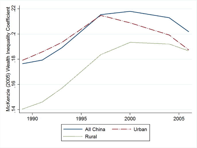
Household Wealth Inequality Over Time

Several important observations can be made from this figure. First, consistent with what is generally observed with respect to income inequality in China, this figure suggests that asset wealth inequality rose substantially through the mid- to late-1990s. Second, while relative inequality was higher in urban areas during this time, the rate of increase in inequality was higher in rural areas, again generally consistent with most evidence regarding patterns of income inequality. However, unlike most studies of income inequality in China, this suggests that asset wealth inequality peaked in roughly the year 2000, and has consistently declined with the passage of time since then. The reduction in nation-wide asset wealth inequality was precipitated by a significant decline in wealth inequality among urban residents, beginning in the late-1990s. Not only did reductions in asset wealth inequality begin earlier in urban areas than in rural areas, but inequality has declined at a faster pace in urban areas. By the end of the sample period, asset wealth inequality in urban areas was roughly the same as that in rural areas. Given that urban development is significantly ahead of rural development, these results suggest that the widespread sharing of improvements in basic infrastructure were felt sooner in urban areas. As rural development occurred later than urban development, it took longer for the benefits to be more widespread. Asset wealth inequality throughout China is higher than in either rural or urban areas, primarily due to urban-rural asset wealth disparities. But asset wealth inequality throughout China has been declining since 2000, capturing both lower inequality within rural and urban areas as well as lower inequality between rural and urban areas. This suggests that the pace of wealth growth in rural areas has been greater than the pace of wealth growth in urban areas, leading to a narrower wealth gap between urban and rural areas. Since W₃ is a mean-zero distribution, we cannot compute growth rates or urban-rural wealth ratios, but casual observation at the evolution of wealth supports the hypothesis that rural wealth growth has been substantially higher than urban wealth growth, and that the resultant narrowing of the urban-rural wealth gap has contributed to lowering wealth inequality in China in recent years.¹⁶ These results appear to support a Kuznets curve in terms of household welfare in China. Over time, clearly the level of household well-being has increased. In the early stages of this process of development, there was an increasing trend in inequality, as the relatively wealthy were able to utilize their pre-existing command over assets and capital to further increase their well-being. After a certain level of development was reached, however, the benefits of development were shared by the relatively poorer members of society, thereby narrowing the welfare gap between the relatively wealthy and the relatively poor.

Many researchers typically find higher income inequality in rural areas compared to urban areas. Since many of the early reforms were in rural organization, these studies often suggest that the reforms benefited some households more than others. Studies rarely suggest that inequality within rural and urban areas have been falling in recent years. Ravallion and Chen (2007) find rising income inequality in both rural and urban areas, with rural areas suffering from a greater degree of inequality than urban areas, suggesting that the rising income inequality has dampened the poverty-reducing impacts of economic growth. We cannot address this issue directly, since we do not have a wealth poverty line with which to make objective comparisons. Nevertheless, we can also use wealth data to create wealth “parade” diagrams in the spirit of the income “parade” diagrams introduced by Pen (1971). To do so, we take the wealth measurements for each survey wave and rank them from lowest to highest and plot these against the proportion of the population that these observations represent. The wealth “parades” for each of the seven survey waves are shown in Figure 3. Contrary to what is typically found when these diagrams are constructed for income distributions, these figures do not reveal a “mass of dwarfs and only a few giants”, indicative of a large share of household wealth being held by a relatively small share of the population. Rather, these figures suggest an extraordinarily wide participation in the ownership of assets, which we take to be indicative of a generally wide command over capabilities and functionings. Even early in the survey, during a period in which economic reforms were viewed as stalling, virtually no one in the population was without at least some wealth. In addition, these figures clearly illustrate that more wealth is being held by the “poorer” members of society over time, as indicated by the upward movement in these distribution functions in successive waves. These trends permit some rather unambiguous conclusions regarding intertemporal social welfare comparisons. The fact that the “parade” diagram for the j^th distribution lies everywhere above the diagram for every other i < j distribution implies successive first-order welfare dominance (Saposnik, 1981) of one wealth distribution over the prior wealth distribution. Hence, these results imply that that social welfare is unambiguously increasing over time.¹⁷ Second, we can make judgments regarding poverty headcount dominance (Foster and Shorrocks, 1988). Since we are dealing with an index, and furthermore since this index is constructed from indicators of physical asset ownership, defining a poverty line by which to compute headcounts or poverty gaps is rendered virtually infeasible. Nevertheless, we can make statements regarding comparisons between the various survey wave’s wealth distributions and a common, arbitrarily defined poverty line. Since the wealth “parade” diagrams for subsequent years lie above and to the left of the “parade” diagrams for all previous years, we know that an increasing proportion of the population has at least a given level of household wealth. For any common wealth poverty line, therefore, the poverty headcount in any particular year is less than the poverty headcount for any and all prior years. If we could define a common poverty line, we would observe a clear trend of declining wealth poverty. While we cannot define such a poverty line we can still appeal to the poverty headcount dominance of subsequent wealth distributions to point to improved social well-being. These results clearly suggest that Chinese households are better off (as of 2006) than they were in 1989.

Figure 3.

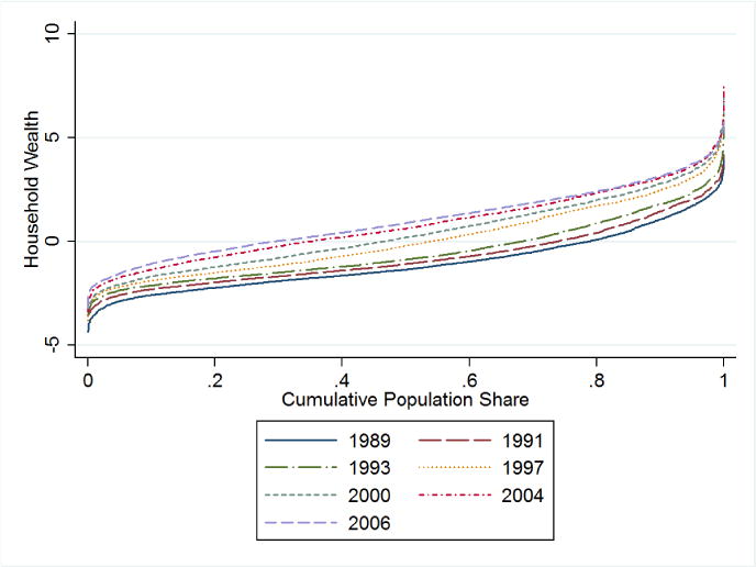
Evolution in the Scope and Distribution of Household Wealth Over Time: Wealth Parade

6 Conclusion

In this paper we have proposed a series of wealth-based measures that incorporate important dimensions of well-being which we suggest are more representative of long-term household well-being, since they are based on ownership of assets and other forms of capital that are representative of a household’s underlying capabilities or opportunities. Since these measures capture dimensions of household socioeconomic status omitted from traditional income- or expenditure-based measures, they can be viewed as complementing these traditional measures. Specifically, we have proposed three measures: a measure based on subjective wealth valuations; an equal-weight wealth index; and, finally, a wealth index whose weights are constructed by performing polyserial PCA on the raw underlying indicators. We have discussed the weaknesses of each of these measures, and have argued that the wealth index constructed using polyserial PCA most completely reflects household well-being and allows for the richest intra- and inter-temporal comparisons. While this measure exhibits modest external consistency with rankings and quintile classifications obtained by traditional income or expenditure measures, the imperfect relationship between these two measures suggest the degree to which our proposed wealth measure captures significantly different information about household welfare than the more traditional measures, thus supporting its role as a complementary measure of household socioeconomic status.

We use our preferred measure to examine patterns of well-being and inequality across both time and the rural/urban divide. Consistent with trends in income, which have shown steadily declining poverty headcounts, we demonstrate that wealth has been steadily increasing over time. In addition, we have demonstrated that wealth has grown faster in rural areas than in urban areas, leading to a decline in the divide between rural and urban asset wealth. We have shown that asset wealth inequality has been declining throughout China since at least 2000, including within both urban and rural areas. Taken in tandem with results on income inequality derived from traditional measures, these results suggest a somewhat more optimistic trend: while income inequality has widened in the wake of economic reforms, there is a more even distribution of basic economic opportunities, suggesting that many of the benefits of these market-oriented reforms have been widely shared. Finally, using wealth “parade” diagrams, we have shown that the wealth distributions in each successive survey wave have improved upon previous years, both in terms of social welfare and wealth poverty.

This work suggests several avenues for future research. Our preferred wealth index explains less than one-fourth of the total variation in underlying, unobserved household well-being, which suggests a significant realm for improvement in the specification of the variables that should be included in any such wealth index. In this application, while we have attempted to be inclusive of many forms of capital, we have focused on various forms of physical capital. If these measures are to be representative of a household’s command over physical, social, and human capital, and indicative of underlying capabilities, then perhaps such an index should consider other dimensions that perhaps are not as tangible as the variables included in our measure. While we have suggested that income or expenditures should not be our primary focus when assessing well-being, it is hard to argue that greater income generally expands a household’s opportunities. Future work could assess the effects of incorporating income or consumption expenditures as simply one among a number of other indicators in such an index. In addition, in constructing our factor weights, we have focused on those weights generated by the first principal component, ignoring higher-order principal components. While this was primarily motivated by previous implementations of this methodology, it was also motivated by the ease with which the first principal component can be interpreted and the difficulties associated with interpreting or incorporating higher-order principal components. Future researchers could identify a reasonable interpretation for second principal components that would increase the applicability of these higher-order principal components for constructing a wealth index like we have attempted here.

References

- Ainsworth M, Filmer D. Inequalities in Children’s Schooling: AIDS, Orphanhood, Poverty, and Gender. World Development. 2006;34:1099–1128. [Google Scholar]
- Bhalla A. Rural-Urban Disparities in India and China. World Development. 1990;18:1097–1110. [Google Scholar]
- Bollen K, Glanville J, Stecklov G. Economic Status Proxies in Studies of Fertility in Developing Countries: Does the Measure Matter? Population Studies. 2001;56:81–96. doi: 10.1080/00324720213796. [DOI] [PubMed] [Google Scholar]
- Case A, Paxson C, Ableidinger J. Orphans in Africa: Parental Death, Poverty, and School Enrollment. Demography. 2004;41:483–508. doi: 10.1353/dem.2004.0019. [DOI] [PubMed] [Google Scholar]
- Deaton A. The Analysis of Household Surveys: A Microeconometric Approach to Development Policy. Johns Hopkins Press: Baltimore; 1997. [Google Scholar]
- Deaton A, Zaidi S. Living Standard Measurement Study Working Paper 135. The World Bank: Washington, D.C; 2002. Guidelines for Constructing Consumption Aggregates for Welfare Analysis. [Google Scholar]
- Fay M, Leipziger D, Wodon Q, Yepes T. Achieving Child-Health-Related Millennium Development Goals: The Role of Infrastructure. World Development. 2005;33:1267–1284. [Google Scholar]
- Filmer D. Fever and its Treatment Among the More and Less Poor in Sub-Saharan Africa. Health Policy and Planning. 2005;20:337–346. doi: 10.1093/heapol/czi043. [DOI] [PubMed] [Google Scholar]
- Filmer D, Pritchett L. Policy Research Working Paper 1994. Development Economics Research Group, The World Bank; Washington, D.C: 1998. Estimating Wealth Effects Without Expenditure Data–Or Tears: An Application to Educational Enrollments in States of India. [DOI] [PubMed] [Google Scholar]
- Filmer D, Pritchett L. Estimating Wealth Effects Without Expenditure Data–Or Tears: An Application to Educational Enrollments in States of India. Demography. 2001;38:115–132. doi: 10.1353/dem.2001.0003. [DOI] [PubMed] [Google Scholar]
- Foster J, Greer J, Thorbecke E. A Class of Decomposable Poverty Measures. Econometrica. 1984;52:761–766. [Google Scholar]
- Foster J, Shorrocks A. Poverty Orderings. Econometrica. 1988;56:173–177. [Google Scholar]
- Friedman M. A Theory of the Consumption Function. Princeton University Press; Princeton, NJ: 1957. [Google Scholar]
- Hussain A, Lanjouw P, Stern N. Income Inequalities in China: Evidence from Household Survey Data. World Development. 1994;22:1947–1957. [Google Scholar]
- Kolenikov S, Angeles G. Socioeconomic Status Measurement with Discrete Proxy Variables: Is Principal Component Analysis a Reliable Answer? Review of Income and Wealth. 2009;55:128–165. [Google Scholar]
- Kung J, Lee Y. So What if There is Income Inequality? The Distributive Consequence of Nonfarm Employment in Rural China. Economic Development and Cultural Change. 2001;50:19–46. [Google Scholar]
- Lin J, Cai F, Li Z. The China Miracle: Development Strategy and Economic Reform. Chinese University Press: Hong Kong; 2003. [Google Scholar]
- McKenzie D. Measuring Inequality with Asset Indicators. Journal of Population Economics. 2005;18:229–260. [Google Scholar]
- Moser C, Felton A. The Construction of an Asset Index Measuring Asset Accumulation in Ecuador. Chronic Poverty Research Center Working Paper. 2007;87 [Google Scholar]
- Olsson U. Maximum Lkelihood Estimation of the Polychoric Correlation Coefficient. Psychometrika. 1979;44:443–460. [Google Scholar]
- Onwujekwe O, Hanson K, Fox-Rushby J. Some Indicators of Socio-Economic Status May Not be Reliable and Use of Indices with these Data Could Worsen Equity. Health Economics. 2006;15:639–644. doi: 10.1002/hec.1071. [DOI] [PubMed] [Google Scholar]
- Pearson K. On the Correlation of Characters Not Qualitatively Measureable. Philosophical Transactions of the Royal Society of London Series A, Containing Papers of a Mathematical or Physical Character. 1900;195:1–47. [Google Scholar]
- Pearson K, Pearson E. On Polychoric Coefficients of Correlation. Biometrika. 1922;14:127. [Google Scholar]
- Pen J. Income Distribution: Facts, Theories, Policies. Allen Lane: London; 1971. [Google Scholar]
- Ravallion M, Chen S. China’s (Uneven) Progress Against Poverty. Journal of Development Economics. 2007;82:1–42. [Google Scholar]
- Sahn D, Stifel D. Poverty Comparisons Over Time and Across Countries in Africa. World Development. 2000;28:2123–2155. [Google Scholar]
- Sahn D, Stifel D. Exploring Alternative Measures of Welfare in the Absence of Expenditure Data. Review of Income and Wealth. 2003;49:463–489. [Google Scholar]
- Saposnik R. Rank Dominance in Income Distributions. Public Choice. 1981;36:147–151. [Google Scholar]
- Sastry N. Trends in Socioeconomic Inequalities in Mortality in Developing Countries: The Case of Child Survival in São Paulo, Brazil. Demography. 2004;41:443–464. doi: 10.1353/dem.2004.0027. [DOI] [PubMed] [Google Scholar]
- Sen A. Commodities and Capabilities. Oxford University Press; New York: 1987. [Google Scholar]
- Sen A. Development as Freedom. Oxford University Press; New York: 1999. [Google Scholar]
Associated Data
This section collects any data citations, data availability statements, or supplementary materials included in this article.