Predicting Gene Function From Patterns of Annotation

Abstract

The Gene Ontology (GO) Consortium has produced a controlled vocabulary for annotation of gene function that is used in many organism-specific gene annotation databases. This allows the prediction of gene function based on patterns of annotation. For example, if annotations for two attributes tend to occur together in a database, then a gene holding one attribute is likely to hold the other as well. We modeled the relationships among GO attributes with decision trees and Bayesian networks, using the annotations in the Saccharomyces Genome Database (SGD) and in FlyBase as training data. We tested the models using cross-validation, and we manually assessed 100 gene–attribute associations that were predicted by the models but that were not present in the SGD or FlyBase databases. Of the 100 manually assessed associations, 41 were judged to be true, and another 42 were judged to be plausible.

[Detailed lists of hypotheses including the curators' comments on each hypothesis, are available at http://llama.med.harvard.edu/∼king/predictions.html.]

The Gene Ontology Consortium (Gene Ontology Consortium 2000) provides a standardized vocabulary for the annotation of gene attributes, which fall into the three general categories of molecular function, biological process, and cellular component. Organism-specific databases such as FlyBase (FlyBase Consortium 2002), Saccharomyces Genome Database (SGD; Cherry et al. 1998), Mouse Genome Database (MGD; Blake et al. 2002), and WormBase (Stein et al. 2001), have codeveloped this vocabulary, and have used it to annotate genes with the attributes that the biomedical literature asserts that they hold.

These databases are incomplete because there are genes whose attributes are not yet all known, and because there is literature that has not yet been digested by the database curators. In such cases it is useful to have a prediction of whether a gene has a certain attribute. Such predictions can help to make the databases more complete (and consequently more useful to researchers) by directing curators toward literature that they may have overlooked. Also, predictions that are not presently supported by the literature provide new hypotheses that may be tested experimentally.

A variety of approaches for predicting Gene Ontology (GO) attributes have been attempted. Natural language processing was used in Raychaudhuri et al. (2002) to automate the curator's task of extracting gene–attribute associations from literature abstracts. Others have assigned attributes to genes on the basis of microarray data (Hvidsten et al. 2001) or protein folds (Schug et al. 2002). These approaches are especially valuable for assigning attributes to genes with otherwise unknown function. But once some attributes of a gene are known, statistical patterns among the annotations themselves can be useful for predicting additional attributes. In this paper, we model the probabilistic relationships between the GO annotations using two approaches, one based on decision trees and the other based on Bayesian networks. We assess the models using cross-validation on the SGD and FlyBase databases. We also manually assess 100 of those gene–attribute associations that the models indicate are likely to hold but that have not been annotated in the databases.

RESULTS

We downloaded the files containing the three branches of the Gene Ontology (GO) and the lists of SGD and FlyBase annotations from http://www.geneontology.org. These files are updated frequently; the versions we used are from January 22, 2002. From these, we constructed a matrix Z for each organism, where Z(i,j) = 1 if gene i is associated with attribute j in the database and Z(i,j) = 0 otherwise. The set of attributes listed in the GO is organized as a directed acyclic graph (DAG)—this is like a hierarchy in which GO terms are subdivided into increasingly detailed or specific child terms; it differs from a hierarchy in that terms may have multiple parents, not just multiple children. An edge from attribute j to attribute k means that k is an instance of attribute j or a component of attribute j, so that any gene associated with attribute k is also associated with attribute j.

The gene association files usually contain explicit annotations only at the most detailed levels that are supported by the literature, but in constructing Z we also include those associations logically implied by the GO DAG. Thus, Z(i,j) = 1 if gene i is explicitly annotated as having attribute j or any of the descendants of attribute j in the GO DAG. We excluded annotations for the three attributes “biological process unknown,” “molecular function unknown,” and “cellular component unknown,” although in principle these are semantically different from the lack of any annotations, because they indicate that someone has looked (Gene Ontology Annotation Guide; http://www.geneontology.org/doc/GO.annotation.html).

There are roughly 13,000 attributes in the GO DAG, but for any given organism only a subset A₁ of them is used. We further restricted our attention to the subset A₁₀ of those attributes that at least 10 genes were annotated as holding, because the probabilistic relationships between these attributes might be estimated with greater confidence. The approach taken in this paper is to use some of the attributes in A₁₀ to predict other attributes in A₁₀.

Let X_j be an indicator random variable for the attribute j ∈ A₁₀, with X_j(i) = 1 if gene i is annotated as having j and X_j(i) = 0 otherwise. [Note that X_j(i) = Z(i,j).] Let nad(X_j) denote the vector consisting of all those random variables X_k ∈ A₁₀ for which k ≠ j and k is neither an ancestor nor a descendant of j in the GO DAG; and let nad(X_j)(i) denote the vector of the values of these random variables for the gene i.

We used standard machine learning techniques (described in the Methods section) to construct, for each attribute j, models M_DT (using decision trees) and M_BN (using Bayesian networks) for the probability that a gene i is annotated as having attribute j, given knowledge of the other attributes that gene i is annotated as holding, excluding attributes that are ancestors or descendants of attribute j in the GO DAG. That is, we constructed models M_DT and M_BN for Pr(X_j | nad(X_j)), which we use for making predictions. (The motivation for ignoring ancestors and descendants when making predictions is discussed in the Manual Assessment section below.) Our approach may be viewed as a supervised-learning approach to pattern recognition, in contrast to unsupervised methods such as clustering; other supervised approaches that might be fruitful, but which we have not evaluated, include support vector machines and artificial neural networks.

Cross-Validation

We assessed our models using 10-fold cross-validation on the SGD and FlyBase databases. This was done separately for the two organisms, and in what follows we use ORG to refer to a generic organism, either fly or yeast. First, from among the set A₁₀ of attributes with at least 10 associated ORG genes, we selected a subset T of the most specific attributes in A₁₀ to be used for the assessment. (See the Methods section for the precise selection criteria.) Then the set G of genes for ORG was randomly partitioned into 10 sets of equal size (±1). For each of the 10 sets of genes, we built models M_DT and M_BN using the remaining nine sets (combined together) as training data. Then for each gene i in the held-out set, we used these models to compute

for each test attribute j in T. (The score q(i,j) may be interpreted as the probability that a gene is annotated with attribute j, given that its other annotations, ignoring those for attribute j and its ancestors and descendants in the GO DAG, agree with those for gene i.)

The scores q(i,j) for each of the 10 folds of the cross-validation were pooled together, and for each threshold t ∈ [0, 1] we computed the true-positive rate

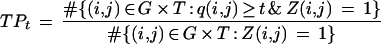and the false-positive rate

Figure 1 shows Receiver Operating Characteristic (ROC) curves, plotting TP_t versus FP_t, for models M_DT and M_BN. For comparison, we have also included the ROC curve for a model M_IND in which attributes are treated as independent, so that q(i,j) is just the fraction of the genes in the training set that are annotated as having attribute j.

Figure 1.

ROC curves for SGD (above) and FlyBase (below), using models M_DT, M_BN, and M_IND. On the left are the entire ROC curves, and on the right are details of the ROC curves at low false-positive rates, with the axes rescaled. (Note that in the graphs on the right, the curves for M_IND are not missing; they are just very close to the horizontal axis.)

There were 6403 genes listed in the SGD association file, and there were 634 attributes that were associated with at least 10 of the genes; 170 of these attributes were in our test set T. Thus there were a total of 6403 × 170  = 1,088,510 examples (i,j) in the set G × T. Of these, 4250 were positive (i.e., had Z(i,j) = 1), and the remaining 1,084,260 were negative. At the point on the ROC curves where the true-positive rate is 0.5 (i.e., where 2125 of the 4250 positive examples are correctly classified as such), 51 of the negative examples were misclassified by M_DT, 143 by M_BN, and 261,003 by M_IND.

There were 7039 genes listed in the FlyBase association file, and there were 794 attributes that were associated with at least 10 of the genes; 218 of these attributes were in our test set T. We included in G another 6461 genes with no annotations, to bring the total number of genes in G to 13,500, an estimate for the total number of Drosophila genes (FlyBase Consortium 2002). Thus, there were a total of 13,500 × 218 = 2,943,000 examples (i,j) in the set G × T. Of these, 5360 were positive and the remaining 2,937,640 were negative. At the point on the ROC curves where the true-positive rate is 0.5 (i.e., where 2680 of the 5360 positive examples are correctly classified as such), 382 of the negative examples were misclassified by M_DT, 684 by M_BN, and 602,178 by M_IND.

Manual Assessment

Although the cross-validation performed above demonstrates that GO annotations may often be predicted accurately on the basis of other annotations, this would be of little use if the organism-specific databases were already saturated, that is, if every genuine gene–attribute association were already annotated. But the databases as they stand now almost certainly contain both errors of inclusion (instances where Z(i,j) = 1 although gene i does not in fact have attribute j), and errors of omission (instances where Z(i,j) = 0 although gene i really does have attribute j). The GO does in fact define a NOT flag for “negative evidence”—evidence that a gene does not hold an attribute—but in the association files from January 22, 2002, the NOT flag was not used at all in the SGD, and only about 30 times in FlyBase.

Because of the large-scale uncertainty about the truth, we have not attempted to explicitly model the truth of whether a gene has an attribute, but have contented ourselves with modeling the patterns among the annotations themselves. Nonetheless, those gene–attribute pairs (i,j) for which Z(i,j) = 0 and q(i,j) is large should be good candidates for errors of omission.

This approach is formally quite similar to approaches used for preference prediction in collaborative filtering (see, e.g., Breese et al. 1998). In a typical application, a model built from a database of customer purchases is used to predict whether customer i would like product j (which he has not purchased), based on the probability that a customer with the same pattern of purchases as customer i (aside from product j) has purchased product j. If this probability is high, a targeted advertisement for product j could be shown to customer i.

We are doing something analogous, with genes playing the role of customers, GO attributes playing the role of products, and annotations playing the role of purchases. Annotations are used as an imperfect proxy for true gene–attribute associations, just as purchases are used as an imperfect proxy for true customer preferences.

Consumer products do not generally have an analog of the GO DAG, however. Our motivation for not considering ancestors or descendants of an attribute j in the GO DAG when predicting attribute j is this: If there is an error of omission for gene i having attribute j, then because of the way annotations are logically propagated up the GO DAG, there are likely to also be errors of omission for gene i having other attributes that are ancestors or descendants of j. Because these attributes can be misleading when we are trying to predict whether Z(i,j) = 0 represents an error of omission, we ignore them.

To test this approach, in the process of doing the cross-validation we also compiled for each organism a list of the 50 gene–attribute pairs (i,j) ∈ G × T that had the highest scores q(i,j), among just those pairs with Z(i,j) = 0. (We used the q scores from M_DT, because judging from the ROC curves it outperformed M_BN at low false-positive rates.) Each list may be thought of as containing 50 hypotheses of the form “gene i is associated with attribute j.”

A FlyBase curator (R.E.F.) assessed the 50 hypotheses for fly, and an SGD curator (S.S.D.) assessed the 50 hypotheses for yeast. The curators gave each hypothesis a rating of 1, 2, or 3, with a rating of 1 meaning that the hypothesis is “known to be true” (despite not being listed in the organism-specific database), 2 meaning “known to be false,” and 3 meaning “neither of the above.” The lists of hypotheses, along with the curators' ratings, are given in Tables 1 and 2. In these tables, and elsewhere in this paper, we prefix the names of GO attributes from the biological process branch with “P,” from the cellular component branch with “C,” and from  the molecular function branch with “F.” More detailed  lists, which include the curators' comments on each hypothesis, are avail− able at http://llama.med.harvard.edu/∼king/predictions.html. Below we summarize the number of hypotheses that received each rating.

Table 1.

Top 50 Hypotheses for FlyBase Using Model M_DT, Sorted Alphabetically by GO Attribute

Rating	Gene name	GO attribute
1	Pros28.2	C-20S core proteasome
1	CG1268	C-hydrogen-transporting ATPase V0  domain
2	CG1268	C-hydrogen-transporting ATPase V1  domain
3	CG5235	C-microsome
3	CG7495	C-microsome
3	Cyp12a2	C-microsome
3	Cyp450_U5csm	C-microsome
3	Tbh	C-microsome
1	CG1909	C-nicotinic acetylcholine-gated  receptor-channel
3	Thor	F-antibacterial peptide
1	Dhc1	F-dynein ATPase
3	syd	F-dynein ATPase
3	Unc-76	F-dynein ATPase
1	bip2	F-general RNA polymerase II  transcription factor
2	Hsf	F-heat shock protein
3	Ubi-p63E	F-heat shock protein
1	cnn	F-myosin ATPase
3	CG4536	F-olfactory receptor
3	lush	F-olfactory receptor
3	TyrR	F-olfactory receptor
1	CG6905	F-pre-mRNA splicing factor
3	REG	F-proteasome endopeptidase
3	Tl	F-scavenger receptor
3	CG4980	F-small nuclear ribonucleoprotein  (now obsolete)
3	CG6905	F-small nuclear ribonucleoprotein  (now obsolete)
2	CG4980	F-small nuclear RNA (now obsolete)
2	CG6905	F-small nuclear RNA (now obsolete)
1	bnk	F-structural protein of cytoskeleton
1	Cortactin	F-structural protein of cytoskeleton
1	CG12740	F-structural protein of ribosome
1	CG12775	F-structural protein of ribosome
3	PK11	F-taste receptor
3	PK19	F-taste receptor
3	Voila	F-taste receptor
2	CG4415	F-transfer RNA (now obsolete)
1	trp&ggr	P-calcium ion transport
1	Ulp1	P-deubiquitylation
1	Cdic	P-microtubule-based movement
3	CG10845	P-microtubule-based movement
3	CG1193	P-microtubule-based movement
1	kl-2	P-microtubule-based movement
3	shi	P-microtubule-based movement
3	unc-104	P-microtubule-based movement
1	CG14060	P-mRNA splicing
1	CG4980	P-mRNA splicing
1	CG5931	P-mRNA splicing
1	CG7972	P-mRNA splicing
1	AGO1	P-protein synthesis initiation
1	CG12413	P-protein synthesis initiation
1	1(2)01424	P-protein synthesis initiation

The first column gives the curator's rating of each hypothesis, with 1 meaning “known to be true,” 2 meaning “known to be false,” and 3 meaning “neither of the above.”

Table 2.

Top 50 Hypotheses for SGD Using Model M_DT, Sorted Alphabetically by GO Attribute

Rating	Gene name	GO attribute
3	CUP5	C-actin cortical patch (sensu Saccharomyces)
3	UBC9	C-anaphase-promoting complex
1	SNR18	C-box C + D snoRNP protein (now obsolete)
1	SNR24	C-box C + D snoRNP protein (now obsolete)
3	SNR18	C-box H + ACA snoRNP protein (now obsolete)
2	RRP6	C-cytoplasmic exosome (RNase complex)
2	NHX1	C-hydrogen-translocating V-type ATPase
2	SRB8	C-mediator complex
3	IMG1	C-mitochondrial large ribosomal subunit
3	MRP8	C-mitochondrial large ribosomal subunit
3	YPL183W-A	C-mitochondrial large ribosomal subunit
1	RPM2	C-ribonuclease P
2	CDC9	F-DNA-directed DNA polymerase
1	HXT1	F-fructose transporter
1	ANC1	F-general RNA polymerase II transcription factor
2	VPH2	F-hydrogen-transporting two-sector ATPase
1	DOA4	F-proteasome endopeptidase
2	NSA3	F-proteasome endopeptidase
1	RPN12	F-proteasome endopeptidase
1	RPN13	F-proteasome endopeptidase
1	RPN2	F-proteasome endopeptidase
3	MSP1	F-protein transporter
1	SSC1	F-protein transporter
1	SIN4	F-RNA polymerase II transcription mediator
3	DIM1	F-small nuclear ribonucleoprotein (now obsolete)
2	FMT1	F-translation initiation factor
2	UBI4	F-ubiquitin-specific protease
3	HRB1	P-35S primary transcript processing
1	RAT1	P-35S primary transcript processing
1	SEN1	P-35S primary transcript processing
3	UBP11	P-deubiquitylation
3	CPR4	P-ergosterol biosynthesis
3	CPR5	P-ergosterol biosynthesis
3	HSM3	P-leading strand elongation
3	KAR1	P-microtubule nucleation
2	MPS2	P-microtubule nucleation
2	DPB4	P-mismatch repair
2	TOM71	P-mitochondrial translocation
1	SPC72	P-mitotic chromosome segregation
3	UBC9	P-mitotic metaphase/anaphase transition
1	UBC9	P-mitotic spindle elongation
1	CLF1	P-mRNA splicing
3	NDC1	P-mRNA-nucleus export
3	SEC1	P-polar budding
1	BUB1	P-protein amino acid phosphorylation
1	IRE1	P-protein amino acid phosphorylation
1	VPS15	P-protein amino acid phosphorylation
3	SNR30	P-rRNA modification
2	IDP1	P-tricarboxylic acid cycle
3	ASM4	P-tRNA-nucleus export

The first column gives the curator's rating of each hypothesis, with 1 meaning “known to be true,” 2 meaning “known to be false,” and 3 meaning “neither of the above.”

These results indicate that our success rate was between 44% and 90% for the 50 FlyBase hypotheses, and between 38% and 76% for the 50 SGD hypotheses.

DISCUSSION

ROC Analysis

For a perfect classifier, there would be a threshold t for which TP_t = 1 and FP_t = 0. The ROC curve for such a classifier would climb up the line FP = 0 until it reached this point, and would then follow the line TP = 1 until it reached the point with TP = 1 and FP = 1.

For a method that assigns scores q(i,j) completely at random, the expected ROC curve would be a diagonal line from the point with FP = 0 and TP = 0 to the point with FP = 1 and TP = 1. (The model M_IND performs better than this because it assigns higher q scores for more commonly occurring attributes.)

It is not possible to perfectly predict whether a gene i is annotated as having attribute j solely on the basis of the other annotations held by gene i, because there are often many genes that have exactly the same combination of annotations aside from j, some of which are also annotated as having attribute j and some of which are not. For example, nearly half the genes in the SGD have no annotations whatsoever, once those for “biological process unknown,” “molecular function unknown,” and “cellular component unknown” are removed; another one-sixth of the genes have exactly one explicit annotation (together with the annotations implied by this via the GO DAG). These annotations are difficult to predict: suppose a gene's only explicit annotation is for attribute j. Then when trying to predict whether gene i has attribute j without looking at j or its ancestors or descendants in the GO DAG, the gene looks exactly like the 3000 or so genes that have no annotations whatsoever, so the score q(i,j) is low.

Of the 4250 SGD gene–attribute pairs (i,j) ∈ G × T for which Z(i,j) = 1, 315 were such that gene i had no annotations among the attributes in nad(X_j). This explains why the slope of the ROC curves for SGD (using models M_DT and M_BN) decrease sharply before a true-positive rate of 93% is reached. Similar reasoning explains why the slopes of the ROC curves for FlyBase decrease sharply before a true-positive rate of 78% is reached. (The ROC curves obtained by computing q(i,j) only when gene i has at least one annotation for an attribute in nad(X_j) are available at http://llama.med.harvard.edu/∼king/predictions.html.)

Note that for both FlyBase and SGD, M_DT outperforms M_BN at low false-positive rates, but eventually M_BN gains the advantage. The crossover point for SGD is at a false-positive rate of ∼0.02 (corresponding to ∼20,000 false positives), and the crossover point for FlyBase is at a false-positive rate of ∼0.05 (corresponding to ∼150,000 false positives).

Discussion of Manual Assessment

In assessing our hypotheses, the GO curators availed themselves of all information at their disposal, including the other GO annotations for the genes, annotations for homologous genes in other organisms, FlyBase and SGD internal notes, data from InterPro (Apweiler et al. 2000), and relevant papers.

Below we give examples of FlyBase hypotheses that were rated 1, 2, and 3, along with the curator's rationale for assigning these ratings.

1. Known to be true: The hypothesis that the gene with FlyBase accession ID CG1909 has the GO attribute “C-nicotinic acetylcholine-gated receptor-channel.” The gene CG1909 is annotated as having the function “F-nicotinic acetylcholine receptor-associated protein,” from which the hypothesized cellular component association follows.

2. Known to be false: The hypothesis that the gene hsf has the GO attribute “F-heat shock protein.” The gene hsf is a transcriptional activator of heat-shock genes. Heat-shock factors are transcription factors that act on the genes that encode heat-shock proteins, but are not chaperones and thus are not themselves heat-shock proteins.

3. Neither of the above: The hypothesis that the gene CG1193 has the GO attribute “P-microtubule-based movement.” CG1193 encodes katanin, a microtubule-severing protein. Although it is possible that it is involved in microtubule transport, there is no definite evidence for this.

In many cases, evaluating these hypotheses led the curators to literature or data sufficient to justify adding the annotation to FlyBase or SGD. This is sometimes attributable to the decision of the GO Consortium to model the three branches of the ontology independently. A consequence of this is that the GO DAG has no edges that connect attributes in different branches. Nonetheless, there are cases in which an attribute in one branch (e.g., molecular function) implies an attribute in another branch (e.g., biological process; Gene Ontology Consortium 2001). Because these interbranch logical relations are not codified in the GO DAG, it is incumbent on the curators to maintain consistency between the branches. If the curators are for the most part successful in this, then these relations (and other probabilistic relations within and between the branches) can be learned by our models, and our models can then flag the isolated instances in which annotations were overlooked. Thus, one immediate application of our methods is the improvement of the gene annotation databases. Aside from a few unusual cases, such as predictions that were for GO attributes that are now obsolete, those predictions rated “known to be true” will be added to FlyBase or SGD.

Another application we envision is that a researcher querying a database for genes with some attribute or combination of attributes may like to supplement the list of perfect matches (of which there may be few or none) with genes that are predicted to hold the attributes. This may be helpful in allocating experimental resources. For each hypothesis we evaluated, <2% of the genes were annotated as having the hypothesized attribute (usually <0.5%), so blindly fishing around for genes that hold these attributes is likely to be unproductive; but >40% of our predictions were judged to be true. The success rate is perhaps much higher, because we do not know whether the hypotheses rated 3 are true or not. The hypotheses rated 3 are perhaps even more interesting than those rated 1, because they may reflect associations that are true but presently unknown, rather than associations that are known but absent from the databases.

In principle, the techniques we used for predicting errors of omission in the databases may also be used to predict possible errors of inclusion, by flagging those existing annotations that have abnormally low q scores. This may be more difficult than predicting errors of omission, however, because the general sparsity of the databases causes many legitimate annotations to have q scores <0.01. We examined 12 of the existing FlyBase annotations that had the lowest q scores, but none appeared to be erroneous. (Here we were looking for errors such as annotations using GO terms not supported by assertations in the literature, rather than errors in the literature itself, which would be harder to assess.)

METHODS

Selection of the Test Attributes

We wanted to assess our predictions on test attributes that were reasonably specific, because a prediction that a gene is associated with a general attribute such as “biological process” is rather uninteresting. We also wanted the test attributes to have no GO edges between them, because using logically dependent test attributes could have the effect of rewarding a single good prediction, or penalizing a single bad prediction, multiple times. With these criteria in mind, we chose the set of test attributes T to consist of all the attributes in A₁₀ that had no descendants in A₁₀, with the additional technical requirement that no attributes j ∈ T and k ∈ A₁₀ may have any common descendant l ∈ A₁, unless k is an ancestor of j. The idea is that, if gene i has attribute j, we should not be allowed to use any direct evidence for this when predicting whether gene i has attribute j during cross-validation. Because we make predictions just on the basis of the random variables in nad(X_j), this is usually not a problem, but sometimes more care is needed because of multiple parentage in the GO DAG. By removing from T any attribute j that violated the technical requirement above, we ensured that no residue of an annotation for an attribute l ever appeared as an annotation for k ∈ nad(X_j) when making a prediction for attribute j.

Decision Trees

See Breiman et al. (1984) or Quinlan (1993) for an overview of decision trees and their applications. For our purposes, the decision tree for attribute j prescribes a sequence of tests to apply to a gene to aid in predicting whether the gene is annotated as having attribute j. The tests are all of the form, “Is the gene annotated as having attribute k?” for some k ≠ j, with k ∈ A₁₀ being neither an ancestor nor a descendant of j in the GO DAG. Which test is applied depends on the result of previous tests—hence the tree structure. (Note that we are using our decision tree to model the conditional probability distribution of X_j given nad(X_j), not just to classify genes as having attribute j or not; some authors use the name “probabilistic decision trees” for trees such as ours.)

We constructed the decision tree for attribute j greedily, by starting with all genes g in the training set in a single root node, and then recursively splitting each node N by testing on the attribute k for which the information gain for attribute j is maximal.

If we test on attribute k, splitting N into N₀ and N₁, where N_t = {g ∈ N : X_k(g) = t}, then the information gain is defined to be

Here H_N(X_j) is the entropy of X_j at node N, which is defined to be −p_N log(p_N) − (1 − p_N) log(1 − p_N), where p_N is the probability that a gene g ∈ G at a node N is annotated as having attribute j (see, e.g., Cover and Thomas 1991). As in Niblett and Bratko (1986), we used the estimate

where p(j) is the fraction of the genes in the entire training set that are annotated as having attribute j and m is an adjustable parameter. The term mp(j) is used as a pseudocount—a small sample-size regularization term, with an interpretation as a prior probability in a Bayesian framework (see, e.g., Ewans and Grant 2001); as our prior convictions about p_N were fairly weak, we set m = 1. We used #{g ∈ N_t}/#{g ∈ N} as an estimate for Pr(g ∈ N_t | g ∈ N) for t = 0 and t = 1, again following Niblett and Bratko (1986).

When no test at a node N provides a positive information gain, the node is not split, but becomes a leaf. It is labeled with the estimate p_N of the probability that a gene at node N has attribute j, as defined above.

A tree grown in this manner will usually overfit the training data, and consequently perform poorly on the held-out test data. A standard way of combating this is to prune away some of the branches after the tree is grown. We used the Bayesian Information Criterion

which is asymptotically equivalent to the Minimum Description Length (MDL; Schwartz 1978) for model selection during pruning (see e.g. Friedman and Goldszmidt 1996). Here K is the number of free parameters in the model (which in our case coincides with the number of leaves in the decision tree), and M is the number of samples in the data set (which in our case is the number of genes in the training set). The first term measures the goodness of fit of the model to the data, and the second term penalizes model complexity. We pruned the tree in a bottom-up fashion, starting at the leaves and working toward the root, pruning away any branch whose removal caused the tree's BIC score to decrease. In computing the BIC score we treated the genes as independent, so that the likelihood Pr(data | model) factored as the product of the likelihood for each gene. (This may not be strictly true, because of homology between genes, for example.)

The score q(i,j) = Pr(X_j = 1 | nad(X_j) = nad(X_j)(i)) was then just p_N, where N is the leaf at which gene i ends up in the decision tree for attribute j.

Figure 2 shows the decision tree for the attribute “C-chromatin,” constructed using the SGD data.

Figure 2.

A decision tree for the attribute “C-chromatin” learned from the SGD data. Starting from the top node, if a gene is annotated with the attribute listed in the node, then it travels down the edge labeled “+”; otherwise it travels down the edge labeled “−.” Leaf nodes are labeled with the number of genes in the training set that end up at the node, split into those that are annotated with “C-chromatin” in the SGD database (prefixed by “+”) and those that are not (prefixed by “−”). Ancestors and descendants of “C-chromatin” in the GO DAG were not allowed for making splits in this tree.

Bayesian Networks

In the approach described above, we constructed a decision tree modeling Pr(X_j | nad(X_j)) independently for each attribute j. An alternative approach is to model the joint probability distribution Pr(X₁, X₂, …, X_N) of all the attributes. From the joint probability distribution, one can compute conditional probabilities such as Pr(X_j | nad(X_j)).

Decision trees assembled independently as in the subsection above are not in general compatible with any single joint distribution (see, e.g., Heckerman et al. 2000), so this alternative approach has the advantage of internal consistency. Another advantage is that from the joint distribution one can also compute predictions for combinations of attributes, rather than just for a single attribute, without relearning the model. One drawback is the increased computational complexity in computing q(i,j).

A Bayesian network (Pearl 1988; Jensen 2001) is a formalism for representing a joint probability distribution as a directed graph, where vertices correspond to random variables and the absence of an edge between vertices indicates a conditional independence between the random variables. Among their many applications, Bayesian networks have been used for medical diagnosis (e.g., Kahn Jr. et al. 1997; Jaakkola and Jordan 1999) and for inferring gene regulatory networks (e.g., Friedman et al. 2000).

By the chain rule of probability, for any ordering X₁, …, X_N of the random variables corresponding to the GO attributes, the joint probability Pr(X₁, …, X_N) factors as

For a Bayesian network, the idea is to exploit conditional independencies between the attributes to find a subset pa(X_j) of {X₁, …, X_j−1} for which Pr(X_j | pa(X_j)) is a good approximation to Pr(X_j | X₁, …, X_j−1). This can greatly reduce the number of parameters that must be estimated.

The extent to which these conditional independencies may be exploited depends on the ordering of the variables. Because the logical relations encoded by the GO DAG induce conditional independencies that we would like to exploit, we chose an ordering of the random variables that is compatible with the GO DAG, that is, an ordering X₁, …, X_N in which j < k whenever X_j is a parent of X_k in the GO DAG. Because the GO DAG is acyclic, such an ordering exists, and is called a linear ordering or a topological sorting of the DAG. (There are, in fact, many topological sortings of the GO DAG; we did not attempt to find an optimal one.)

As in Friedman and Goldszmidt (1996) and Heckerman et al. (2000), we represented the local conditional probability distributions Pr(X_j | pa(X_j)) by probabilistic decision trees rather than by conditional probability tables. This is a more parsimonious representation when there are conditional independencies that hold only for particular values of the random variables in pa(X_j). The decision trees were constructed using the algorithm described in the subsection above, with the following differences.

In the subsection above, when constructing the decision tree for attribute j we allowed splits to be made using any attribute k ≠ j for which k was neither a descendent nor an ancestor of j in the GO DAG; here we allowed splits to be made using any attribute k with k < j in the topological sorting of the GO DAG. This means that none of the descendants of j in the GO DAG could be used for splits, but that all of the ancestors of j in the GO DAG could be used, and usually some other attributes as well. We also modified the decision-tree-growing algorithm slightly so that the first test was: “Is X_k(i) = 1 for all of the parents k of j in the GO DAG?” If the answer was “no,” then it logically follows that X_j(i) = 0, so gene i was sent to a leaf node N with N_p = 0. (Unlike the other nodes, no pseudocounts were used here because X_j(i) = 0 is a logical necessity; this node was also designated unpruneable.) If the answer was “yes,” then the gene was sent to another node, which was then recursively split using the ordinary information gain criterion to complete the tree. This tree was pruned as in the subsection above. The elements of pa(X_j) were just those X_k for which attribute k was used as a split in the pruned decision tree for attribute j.

The graphical representation of the Bayesian network is constructed by including a directed edge from vertex X_k to vertex X_j if and only if X_k ∈ pa(X_j). The elements of pa(X_j) are usually called the parents of X_j; we have not referred to them as such until now, to avoid confusion with the parents of attribute j in the GO DAG. But note that by our choice of an ordering of the attributes, and our modifications to the decision-tree-growing algorithm, we have arranged things so that the GO DAG is a subgraph of the Bayesian network, that is, so that if k is a parent of j in the GO DAG, then X_k ∈ pa(X_j). (The converse need not be true, however.) We have also ensured that the joint probability distribution defined by the Bayesian network is consistent with the logical constraints imposed by the GO DAG.

Figure 3 shows a fragment of the Bayesian network for the SGD attributes.

Figure 3.

A fragment of the Bayesian network for SGD attributes. The full network contains 634 nodes. There is an edge from X_j to X_k if and only if X_j ∈ pa(X_k). Most of the displayed vertices have additional outgoing edges, not shown, to vertices that are not shown. Edges in the Bayesian network that are also edges in the GO DAG are shown in black; the remaining edges are shown in gray.

Computing the joint probability of a specific sequence of annotations X = (X₁, …, X_N) is straightforward with the Bayesian network: Pr(X) factors as ∏Pr(X_j | pa(X_j)), and if a gene with annotation vector X ends up at leaf N in the decision tree for attribute j, then the term Pr(X_j | pa(X_j)) is equal to p_N if X_j = 1, and to 1 − p_N if X_j = 0.

Now Pr(nad(X_j) = nad(X_j)(i)) may be computed by summing the joint probability of X over all possible assignments of values to the random variables not in nad(X_j), keeping the known values of the random variables in nad(X_j) fixed as nad(X_j)(i). The score q(i,j) = Pr(X_j = 1 | nad(X_j) = nad(X_j)(i)) is just the ratio of the sum of those joint probabilities for assignments in which X_j = 1 to the total sum.

Computing this sum using brute force has running time exponential in the number of ancestors and descendants of attribute j in the GO DAG. In our computations, each test attribute j ∈ T had <25 ancestors in A₁₀ and no descendants in A₁₀ (because we were predicting only the most detailed attributes), so the brute force method was feasible. But given that any assignment of values to the random variables not in nad(X_j) that is not logically consistent with the GO DAG has joint probability zero, we were able to speed up the computation by summing over just those assignments that were logically consistent with the GO DAG. An alternative would be to use the variable elimination algorithm or the junction tree algorithm (see Jensen 2001) to speed up the computation. These algorithms are not always practical for large networks with many undirected cycles, such as ours, but because all but 20 or so of the random variables in our network are instantiated with known values when computing q(i,j), this is not a problem.

The Bayesian network approach also has a natural extension in which the reliability of different evidence types is explicitly modeled, and the distinction between negative evidence and the absence of evidence is made explicit. Such a model would have two vertices for each GO attribute: an “evidence” vertex that gives the types of evidence (if any), and a “hidden” vertex corresponding to the truth (which is not directly observable). Learning the topology and parameters of such a model would require a technique that deals with missing data, such as the structural EM algorithm (Friedman 1998). The goal would then be to infer the values of all the hidden variables for a gene on the basis of all the evidence for the gene. But the model would have hundreds of hidden variables to sum over, making exact inference infeasible. (Note that even approximate inference in a general Bayesian network is NP-hard [Cooper 1990; Dagum and Luby 1993].) Nonetheless, there might be some prospect of reasonably estimating the values of the hidden variables using Monte Carlo methods (Gilks et al. 1996) or “loopy” belief propagation (Murphy et al. 1999).

WEB SITE REFERENCES

http://llama.med.harvard.edu/∼king/predictions.html; curators' notes on hypotheses.

http://www.geneontology.org; Gene Ontology Consortium homepage.

http://www.geneontology.org/doc/GO.annotation.html; Gene Ontology Annotation Guide.

Table a.

	FlyBase	SGD
(1) known to be true	22	19
(2) known to be false	5	12
(3) neither of the above	23	19

REFERENCES

- 1.Apweiler R., Attwood, T.K., Bairoch, A., Bateman, A., Birney, E.E., Biswas, M., Bucher, P., Cerutti, L., Corpet, F., Croning, M.D.R., et al. 2000. InterPro: An integrated documentation resource for protein families, domains and functional sites. Bioinfomatics 16: 1145-1150. [DOI] [PubMed] [Google Scholar]
- 2.Blake J.A., Richardson, J.E., Bult, C.J., Kadin, J.A., Eppig, J.T., and the Mouse Genome Database Group 2002. The Mouse Genome Database (MGD): The model organism database for the laboratory mouse. Nucleic Acids Res. 30: 113-115. [DOI] [PMC free article] [PubMed] [Google Scholar]
- 3.Breese J., Heckerman, D., and Kadie, C. 1998. Empirical analysis of predictive algorithms for collaborative filtering. In Proceedings of the 14th Conference on Uncertainty in Artificial Intelligence (eds. G.F. Cooper & S. Moral), pp. 43–52. Morgan Kaufman, San Francisco, CA.
- 4.Breiman L., Friedman, J.H., Olsen, R.A., and Stone, C.J., 1984. Classification and regression trees. Chapman & Hall, New York, NY.
- 5.Cherry J.M., Adler, C., Ball, C., Chervitz, S.A., Dwight, S.S., Hester, E.T., Jia, Y., Juvik, G., Roe, T., Schroeder, M., et al. 1998. SGD: Saccharomyces Genome Database. Nucleic Acids Res. 26: 73-79. [DOI] [PMC free article] [PubMed] [Google Scholar]
- 6.Cooper G.F. 1990. Probabilistic inference using belief networks is NP-hard. Artif. Intell. 42: 393-405. [Google Scholar]
- 7.Cover T.M. and Thomas, J.A., 1991. Elements of information theory. John Wiley, New York, NY.
- 8.Dagum P. and Luby, M. 1993. Approximating probabilistic inference in Bayesian belief networks is NP-hard. Artificial Intelligence 60: 141-153. [Google Scholar]
- 9.Ewans W.J. and Grant, G.R., 2001. Statistical methods in bioinformatics: An introduction. Springer-Verlag, New York, NY.
- 10.The FlyBase Consortium 2002. The FlyBase database of the Drosophila genome projects and community literature. Nucleic Acids Res. 30: 106-108. [DOI] [PMC free article] [PubMed] [Google Scholar]
- 11.Friedman N. 1998. The Bayesian structural EM algorithm. In Proceedings of the 14th Conference on Uncertainty in Artificial Intelligence (eds. G.F. Cooper & S. Moral), pp. 129–138. Morgan Kaufmann, San Francisco, CA.
- 12.Friedman N. and Goldszmidt, M. 1996. Learning Bayesian networks with local structure. In Proceedings of the 12th Conference on Uncertainty in Artificial Intelligence (eds. E. Horvitz & F.V. Jensen), pp. 252–262. Morgan Kaufmann, San Francisco, CA.
- 13.Friedman N., Linial, M., Nachman, I., and Pe'er, D. 2000. Using Bayesian networks to analyse expression data. J. Comput. Biol. 7: 601-620. [DOI] [PubMed] [Google Scholar]
- 14.The Gene Ontology Consortium 2000. Gene ontology: Tool for the unification of biology. Nat. Genet. 25: 25-29. [DOI] [PMC free article] [PubMed] [Google Scholar]
- 15.___, 2001. Creating the gene ontology resource: Design and implementation. Genome Res. 11: 1425-1433. [DOI] [PMC free article] [PubMed] [Google Scholar]
- 16.Gilks W.R., S. Richardson & D.J. Spiegelhalter, 1996. Markov chain Monte Carlo in practice. Chapman & Hall, London, UK.
- 17.Heckerman D., Chickering, D., Meek, C., Rounthwaite, R., and Kadie, C. 2000. Dependency networks for inference, collaborative filtering, and data visualization. J. Machine Learn. Res. 1: 49-75. [Google Scholar]
- 18.Hvidsten T.R., Komorowski, J., Sandvik, A.K., Lægreid, A., et al. 2001. Predicting gene function from gene expressions and ontologies. In: In Pacific Symposium in Biocomputing (ed. R.B. Altman), pp. 299–310. World Scientific Publishing Co., Singapore. [DOI] [PubMed]
- 19.Jaakkola T.S. and Jordan, M.I. 1999. Variational probabilistic inference and the QMR-DT database. J. Artificial Intell. Res. 10: 291-322. [Google Scholar]
- 20.Jensen F.V., 2001. Bayesian networks and decision diagrams. Springer-Verlag, New York, NY.
- 21.Kahn C.E., Roberts, L.M., Shaffer, K.A., and Haddawy, P. 1997. Construction of a Bayesian network for mammographic diagnosis of breast cancer. Comput. Biol. Med. 27: 19-29. [DOI] [PubMed] [Google Scholar]
- 22.Murphy K.P., Weiss, Y., and Jordan, M.I. 1999. Loopy belief propagation for approximate inference: An empirical study. In Proceedings of the 15th Conference on Uncertainty in Artificial Intelligence (eds. K.B. Laskey & H. Prade), pp. 467–475. Morgan Kaufmann, San Francisco, CA.
- 23.Niblett T. and Bratko, I. 1986. Learning decision rules in noisy domains. In Developments in expert systems (ed. M. Bramer), pp. 25–34. Cambridge University Press, Cambridge, UK.
- 24.Pearl J., 1988. Probabilistic reasoning in intelligent systems. Morgan Kaufmann, San Francisco, CA.
- 25.Quinlan J.R., 1993. C4.5: Programs for machine learning. Morgan Kaufmann, San Mateo, CA.
- 26.Raychaudhuri S., Chang, J.T., Sutphin, P.D., and Altman, R.B. 2002. Associating genes with gene ontology codes using a maximum entropy analysis of biomedical literature. Genome Res. 12: 203-214. [DOI] [PMC free article] [PubMed] [Google Scholar]
- 27.Schug J., Diskin, S., Mazzarelli, J., Brunk, B.P., and Stoeckert, C.J., Jr. 2002. Predicting gene ontology functions from ProDom and CDD protein domains. Genome Res. 12: 648-655. [DOI] [PMC free article] [PubMed] [Google Scholar]
- 28.Schwartz G. 1978. Estimating the dimension of a model. Ann. Statistics 6: 461-464. [Google Scholar]
- 29.Stein L., Sternberg, P., Durbin, R., Thierry-Mieg, J., and Spieth, J. 2001. WormBase: Network access to the genome and biology of Caenorhabditis elegans. Nucleic Acids Res. 29: 82-86. [DOI] [PMC free article] [PubMed] [Google Scholar]