

Abstract
Bacterial cells display both spatial and temporal organization, and this complex structure is known to play a central role in cellular function. Although nearly one-fifth of all proteins in Escherichia coli localize to specific subcellular locations, fundamental questions remain about how cellular-scale structure is encoded at the level of molecular-scale interactions. One significant limitation to our understanding is that the localization behavior of only a small subset of proteins has been characterized in detail. As an essential step toward a global model of protein localization in bacteria, we capture and quantitatively analyze spatial and temporal protein localization patterns throughout the cell cycle for nearly every protein in E. coli that exhibits nondiffuse localization. This genome-scale analysis reveals significant complexity in patterning, notably in the behavior of DNA-binding proteins. Complete cell-cycle imaging also facilitates analysis of protein partitioning to daughter cells at division, revealing a broad and robust assortment of asymmetric partitioning behaviors.
Introduction
The intricate physical organization of the cell plays a central role in many cellular processes, from chromosome replication and segregation to gene expression and protein synthesis. The importance of cellular organization has long been accepted as an essential component of the biology of eukaryotic cells: Subcellular organelles and complex cell morphologies have been observed and studied since the infancy of light microscopy, but systematic investigations into the role of cellular organization in bacterial cell biology awaited the development of tractable techniques of fluorescence labeling and microscopy on sub-micron length scales (Shapiro et al., 2009). Over the last two decades, many compelling examples of bacterial cellular organization have emerged, including the precise positioning of the septum at midcell during cell division (Raskin and de Boer, 1997; Errington et al., 2003; Lutkenhaus, 2007), the role of chromosome organization in cell polarity (Huitema et al., 2006; Lam et al., 2006) and the localization of the chemotaxis receptors to the cell poles (Alley et al., 1992; Maddock et al., 1993). Nevertheless, a global or proteome-wide understanding of the dynamic cellular-scale organization of proteins in bacterial cells remains elusive.
A significant step toward a global understanding of protein localization in bacterial cells has been achieved by the construction of near-complete libraries of fluorescent protein fusions, first in Escherichia coli (Kitagawa et al., 2006) and more recently in Caulobacter crescentus (Werner et al., 2009). Both collections have been imaged by snapshot analysis (single-time-point imaging), which revealed many examples of proteins with nondiffuse localization patterns, e.g. polar, bipolar, ring-like, punctate, etc.
At the same time, in the absence of time-lapse imaging, it is nearly impossible to differentiate between cell-to-cell variation and cell-cycle-dependent localization. We do not yet know the extent to which bacteria can target proteins to specific cellular positions at specific times during the cell cycle. How many distinct spatiotemporal addresses are in rod-shaped bacterial cells and how precise are these addresses? To what extent does typical protein localization vary during the cell cycle? Even for known cellular addresses, e.g. the cell poles, it is not clear whether or not proteins localize to the pole in a stochastic or temporally defined pattern.
To answer these questions and establish a global picture of protein localization dynamics in the bacterial cell, we undertook a genome-scale quantitative characterization of both the spatial localization of proteins and the cell-cycle-dynamics of these localization patterns in the rod-shaped gram-negative bacterium E. coli. To accomplish this goal, we developed an approach that was motivated by a central challenge in the interpretation of time-dependent protein localization data in prokaryotic cells: The stochastic nature of chemical and physical processes on a molecular-scale produces both significant cell-to-cell variation and temporal fluctuations that may have little physiological significance.
By combining high-throughput time-lapse imaging and automated image analysis, we are able to collect hundreds to thousands of complete cell cycles for each protein fusion, allowing us to quantitatively characterize mean protein localization dynamics for nearly every protein that displays nondiffuse localization. Our analysis reveals that even a bacterial cell without obvious morphological complexity can still exhibit robust, reproducible and strikingly diverse complexity in the spatial and temporal structure of protein localization patterns.
To visualize average protein localization and compare localization behaviors between proteins, we define the consensus localization pattern (the mean over single-cell images), which captures both the spatial and temporal structure of protein localization over the entire cell cycle. Hierarchical clustering and principal component analysis (PCA) reveals large groups of proteins with similar localization patterns, many of which are familiar (cytoplasmic, nucleoid, membrane, Z-ring, bipolar, unipolar), but there is significant and reproducible variation within these categories. Detailed analysis of DNA-binding protein localization patterns reveals considerable spatial complexity: Many DNA-binding proteins appear to consistently bind to a small number of sites on the nucleoid. Proteins that are targeted to the cell poles or midcell arrive at these target locations at distinct times, demonstrating considerable temporal complexity in protein localization. Finally, the explicit observation of protein localization throughout the entire cell cycle also facilitates the analysis of protein partitioning between daughter cells at cell division. We find that many proteins are partitioned with strong asymmetry between daughter cells, including the surprising observation of a number of DNA-binding proteins that are preferentially partitioned to the daughter cell with the new cell pole.
Results
Construction of the localization library
To apply quantitative analysis to protein localization dynamics, we began with an existing library of fluorescent fusions: the complete ASKA green fluorescent protein (GFP) fusion library (Kitagawa et al., 2006). To build a dynamic protein localization library, as a first pass we screened the existing collection of ASKA snapshot data by eye to identify those protein fusions that display nondiffuse localization, resulting in a reduced library of 864 fusions. To this collection we added five additional (non-ASKA) fusions of interest that were not represented or known to show aberrant localization in the ASKA collection (SlmA, MukB, MreB, MinD, Ssb), bringing the final library to 869 unique protein fusions, approximately one-fifth of the E. coli proteome. The resulting localization library was reimaged using high-throughput time-lapse fluorescence microscopy with a frame-capture rate of 6–8 min, described in detail in Experimental procedures. Briefly, log-phase cells grown in minimal liquid media were spotted onto large format agarose pads. The pads were then sealed with a coverslip and imaged using a wide-field fluorescence microscope outfitted with an environmental chamber (30°C, doubling time ∼ 60 min). Images were then segmented: processed to identify cell boundaries from the corresponding phase contrast images and linked frame to frame to build cell cycles. Only complete cell cycles, i.e. cells in which both cell birth and division were explicitly observed, were kept for analysis, necessarily precluding filamentous and nongrowing cells. In a typical experiment, hundreds of complete cell cycles are captured for each protein fusion.
The ASKA library has three potential limitations: (i) the fluorescent fusions are expressed from an inducible promoter on a high-copy plasmid, therefore the total protein abundance is greater than the physiological concentration; (ii) GFP typically does not fold properly in the periplasm (Feilmeier et al., 2000), therefore ASKA fusions to periplasmic proteins are often nonfunctional and thus the localization library is biased toward cytoplasmic proteins; and (iii) in addition to the C-terminal GFP fusion, the protein fusions also have an N-terminal histidine tag. Both C- and N-terminal fusions can potentially lead to loss of function and localization, and may even exhibit artifactual localization as the explicit result of the fusions (Swulius and Jensen, 2012).1 To account for the effects of fusion protein concentration on localization behavior, we imaged the entire localization library at two separate induction levels (50 and 500 μM, see Experimental procedures). Most localization patterns (> 70%) were qualitatively robust to protein concentration. Notable exceptions are the cell division proteins FtsZ and FtsA, and ∼ 250 fusions that tend to form polar-localized aggregates (likely inclusion bodies) at the higher induction level. Although this subset of polar-localized aggregates is likely artifactual, the majority of protein fusions in the localization library exhibit a broad range of dynamic yet reproducible localization patterns that are consistent with expected protein function.
It would be ideal to image all fusions under physiological relevant expression levels, but many proteins are not expressed at robust-enough levels to be visible under standard imaging conditions. If these proteins had been expressed from their endogenous promoter, the practical limitations of fluorescence microscopy would lead to bleaching the low numbers of protein in a single exposure, all but precluding the capture of cell-cycle dynamics.
Therefore, in the context of this study where we explicitly attempt to characterize the cell-cycle dynamics of proteins at a genomic scale, the experiment is only tractable with the expression levels used in the study. Given these constraints, the use of the ASKA collection is both expedient and necessary.
Visualization of complete cell cycles
One of the challenges of high-throughput cell-cycle imaging and analysis is visualizing the complete data set in a meaningful way (Sliusarenko et al., 2011). To efficiently visualize our complete cell-cycle data, we organize each individual cell-cycle images sequentially into a single-cell tower image, in which the cell images are arranged vertically with the first frame of the cell cycle at the top and the final frame (prior to division) at the bottom. Furthermore, as the entire cell cycle is captured, each cell image in the single-cell tower can be oriented to place the new cell pole (the pole produced from the previous division) on the right-hand side (Stewart et al., 2005). Figure 1 shows representative single-cell tower images for nine proteins of known function that exhibit a wide array of dynamic localization, e.g. unipolar, bipolar, Z-ring, etc. Each single-cell tower image qualitatively recapitulates known protein localization behavior, although there is significant cell-to-cell variation in cell-cycle-duration, cell size and cell shape between the individual single-cell tower images.
Fig. 1.

Consensus localization patterns and single-cell tower images for proteins HisG, MreB, MinD, UidR, SeqA, H-NS, Tsr, MalI and FtsZ. Single-cell tower images capture protein localization dynamics in single cells. For each protein, 9–15 complete cell cycles are shown in false color. For SeqA, like many proteins in the collection, the single-cell tower images display significant cell-to-cell variation in protein localization, despite qualitative similarities. To visualize average dynamics and to facilitate the quantitative comparison between protein localization patterns, we compute the consensus localization pattern by computing the mean localization pattern over all single-cell data for each protein.
To benchmark the performance of our high-throughput imaging, we used several metrics:
First, we qualitatively compared our time-lapse images with the snapshot images generated in the original ASKA study of 192 proteins. In all cases, these images were consistent with the published results.
For proteins of particular interest to our lab, we compared our images with other localization studies. Our tower images for many proteins, including H-NS, Tsr and FtsZ (Fig. 1), are consistent with previous reports (Sourjik and Berg, 2000; Errington et al., 2003; Wang et al., 2011). Nevertheless, some well-known proteins (MukB, MreB, MinD, Ssb) showed aberrant localization patterns in both our imaging and the original ASKA study, suggesting that the ASKA fusion was not functional. In these cases, we supplemented the ASKA collection with strains that show the accepted localization pattern as described above, although we have not yet supplemented the collection in all cases where we know that the ASKA fusion shows aberrant localization (for example, MinC, MukE).
Finally, we used the localization pattern of number of fusions to benchmark the performance of the segmentation and cell linking. The Z-ring associated protein FtsZ is a useful tool in evaluating the ability of the segmentation algorithm to accurately recognize cell division as the Z-ring is known to rapidly depolymerize from the new cell pole (the pole that originated from the last division, i.e. the center of the mother cell) at the beginning of the cell cycle. Manual inspection of the data revealed that this depolymerization event obviously occurred in the first frame of the cell cycle in 870 out of 974 complete cell cycles inspected. To determine whether the membrane is included in the segmented area, we inspected the single-cell tower images for proteins known to localize near the cytoplasmic membrane. Although the maximum fluorescence intensity is significantly reduced due to localization to the relatively large surface area of the membrane, single-cell tower images of known membrane-associated proteins such as NupG (nucleoside transporter), QseC (sensory histidine kinase), NanT (siliac acid transporter), and NikB (nickel transporter subunit) all show obvious cytoplasmic membrane localization.
Determination of mean localization dynamics
To identify common motifs in protein localization patterns in the presence of significant cell-to-cell variation, we developed a quantitative method for uniformly characterizing mean localization dynamics: For each protein in the collection, the single-cell tower images were computationally interpolated to a reference cell cycle of uniform size and cell-cycle duration, and then the mean and standard deviation of all interpolated single-cell tower images were computed. We refer to the normalized mean image as the consensus localization pattern, shown to the left of each single tower image collection in Fig. 1. This method allows for quantitative comparison between protein localization patterns as well as a measure of cell-to-cell variation. The consensus localization pattern captures many features of the qualitative behavior found in the single-cell tower images, though it is important to note that the consensus localization pattern is not necessarily a representative cell cycle but rather a mean over cell-to-cell variation.
To evaluate the efficacy of consensus localization patterns in the study of localization dynamics, we carefully examined several proteins whose localization had previously been analyzed. To determine if consensus localization patterns could retain the spatial details of the single-cell tower images, we focused on several proteins with specific, well-characterized patterns: FtsZ, SeqA and MinD.
FtsZ, the tubulin-like protein that polymerizes to form the cytokinetic Z-ring, is positioned at midcell with a precision of 2% of cell length (Errington et al., 2003; Lutkenhaus, 2007). For proteins like FtsZ, for which there is minimal cell-to-cell variation in the protein localization, the consensus localization pattern captures a detailed picture representative of the structure in single cells. For instance, the ring-like structure of FtsZ is revealed by bright symmetric foci at midcell (Fig. 1). Furthermore, it is clear from the consensus localization pattern that the radius of the ring contracts at the end of the cell cycle.
Proteins like SeqA (replication initiation regulator), which form punctate foci and short filaments, are not as precisely positioned and thus show more cell-to-cell variation in the single-cell tower images (Fig. 1). Consequently, the consensus localization pattern for SeqA is more representative of the probability that a focus is at a particular location in the cell rather than a representative protein localization pattern for a single cell (Onogi et al., 1999).
A third instructive example is MinD, the ATPase of the min-system, which oscillates between poles with a period of roughly 1 min (Lutkenhaus, 2007). The consensus localization pattern averages over these oscillations, revealing a minimum at midcell, but does not capture the oscillations that occur on a time scale much faster than our frame-capture rate. In conclusion, the consensus localization pattern effectively captures the cell-to-cell mean protein concentration, but some important features are not captured as a consequence of cell-to-cell averaging.
To evaluate the efficacy of the analysis of the consensus localization pattern in determining the timing or ordering of events during the cell cycle, we examined the localization dynamics of two specific cellular processes where the ordering of protein localization has previously been described. In the first example, we analyze the dynamic co-localization of MukB, an SMC-like protein involved in chromosome segregation, and SeqA, a regulator of replication initiation (Hiraga et al., 1989; Lu et al., 1994). This analysis is shown in Fig. 2A. To focus on the long axis positional dynamics, we display mean protein localization as a kymograph. The MukB kymograph shows maxima in fluorescence intensity on either side of midcell throughout the cell cycle, whereas SeqA appears initially centered around midcell, before moving to the quarter cell positions at time 0.7 cell cycles (because the single-cell towers have variable cell-cycle length, the consensus image time must be measured relative to the cell cycle). This conclusion is consistent with previous results (Ohsumi et al., 2001).
Fig. 2.

Cell-cycle timing probed by consensus localization patterns. To demonstrate the ability of consensus localization patterns to determine cell-cycle timing, we analyze the localization patterns of proteins in two processes where the cell-cycle ordering of protein localization is already known. Consensus location patterns are represented as kymographs.
A. SeqA and MukB are proteins implicated in chromosome replication and segregation. Consistent with previously reported results, the kymographs show MukB arriving at the quarter-cell position prior to SeqA.
B. FtsZ, MinD and SlmA are proteins implicated in cytokinesis. Both MinD and SlmA are known to inhibit FtsZ-dependent Z-ring formation. The kymographs show significant FtsZ localization at midcell only after MinD and SlmA are depleted from midcell, consistent with the known mechanism of z-ring regulation.
In the second example, we return to the cytokinetic Z-ring. The MinCDE system (Lutkenhaus, 2007) and SlmA, a nucleoid occlusion factor (Bernhardt and de Boer, 2005), are both inhibitors of Z-ring formation. The kymographs in Fig. 2B both appear to be consistent with the accepted model that the Z-ring forms only after MinD and SlmA are depleted at midcell. Again, these results are consistent with previous detailed analyses, and therefore support the efficacy of the analysis of the consensus localization pattern in determining cell-cycle timing.
Public database for localization data
To allow for efficient visualization and sharing of our dynamic protein localization library, we have developed a publicly accessible online database with all the raw and processed data, as well as analysis scripts, organized in a searchable list (http://mtshasta.phys.washington.edu/localizome). The database is organized by gene name, such that each individual fusion has a unique page with consensus localization patterns for multiple induction conditions, as well as the single-cell tower images and additional analyses for each, which can be easily browsed and downloaded.
Comparison of consensus localization patterns at the genome scale
Although the consensus co-localization technique demonstrated in Fig. 2 works well for the comparison of a small number of proteins, we also want to efficiently compare the localization dynamics for any set of proteins in the collection. To do this, we compute the distance between all consensus localization patterns to generate a distance matrix, shown in Fig. 3 and described in more detail in the Experimental procedures. Briefly, all proteins in the localization library are indexed as rows and columns of a large matrix. The entry in the matrix corresponding to arbitrary proteins A and B (row ‘A’, column ‘B’) is defined as the distance between the proteins, DAB, where distance is calculated by subtracting the two consensus localization patterns from each other, such that similar patterns have distance D = 0 while orthogonal patterns have distance D = 1 (due to normalization). This metric explicitly compares localization throughout the cell cycle. To find proteins with similar dynamic localization patterns to a protein of interest, we find the smallest elements (the shortest distances) in the row corresponding to the protein of interest. The 10 most similar localization patterns for each protein are included in the online database for each protein in the localization library. The proteins are ordered in the matrix by hierarchical clustering to group proteins with similar localization patterns, giving the distance matrix a block-diagonal structure. Blue blocks along the diagonal of the matrix represent groups of proteins with similar localization patterns. For example, proteins IlvE and YneH both appear to form unipolar inclusion bodies that result in nearly identical consensus localization patterns (Fig. 3). Hierarchical clustering groups these proteins together, with others, in cluster with a dark blue diagonal block representing a group of patterns that are both highly similar to each other while significantly distinct from the other patterns in the library. In contrast, DNA-binding proteins UidR (transcriptional repressor), H-NS (global transcriptional regulator) and Ssb (single-stranded binding), which are all known to localize to the nucleoid, all cluster to the top-left corner of the distance matrix.
Fig. 3.
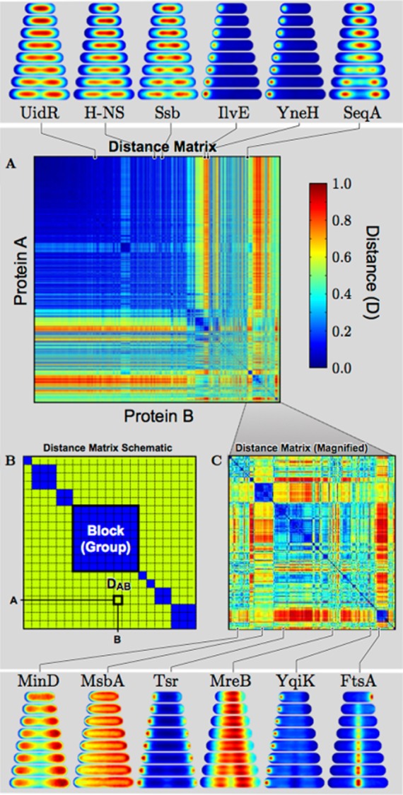
Virtual co-localization of all protein pairs measured by distance between consensus localization patterns.
(A) The distance matrix is visualized as a heat map with (B) schematic representation of block diagonal form and (C) a magnified region of the distance matrix. Consensus localization patterns that are identical have a distance of zero (dark blue, see colorbar). Representative examples of consensus localization patterns and their positions in the distance matrix are shown above and below the matrix.
To evaluate the efficacy of the distance matrix in the comparison of localization patterns, we again examined proteins with previously described spatial and temporal localization patterns. For proteins with relatively distinct consensus localization patterns like FtsZ and SeqA, the top match in the collection of consensus images was the same protein imaged under other induction conditions. After itself, the best match for FtsZ is FtsA, which is known to bind to FtsZ whenever FtsZ is localized (Errington et al., 2003). Both results support the use of the distance matrix in the identification of protein with similar localization patterns.
Day-to-day variation and protein copy-number dependence
Defining the distance between localization patterns permits us to discuss the error in the localization patterns in a quantitative way. For this analysis, we focus on 48 strains from the collection that we imaged multiple times under identical induction conditions. To estimate the error from analyzing a finite number of cells, we divided each single-cell tower data set randomly into two subsets and computed the consensus localization pattern for each subset. The average distance between subsets was D = 0.01 (Note: identical patterns have distance 0 and orthogonal patterns have distance 1). To estimate the day-to-day variation, we computed the distance between two data sets taken under the same induction conditions but on different days. The average distance between matching pairs of proteins was D = 0.03.
To investigate the dependence of localization on the amount of protein in the cell, we compared localization patterns of the ASKA plasmid expression constructs for high (500 μM) and low (50 μM) IPTG induction conditions. The average distance between matching pairs of proteins was D = 0.03, essentially identical to the day-to-day error. Therefore, as we observed qualitatively, protein abundance does not appear to impact the majority of localization patterns.
Classifying localization patterns by PCA
To identify common motifs in protein localization associated with distinct localization mechanisms and cellular functions, we initially attempted to group localization patterns using the sorted distance matrix alone. Although the distance metric is effective at identifying similar localization patterns, it fails to identify distinct groups of localization patterns. An alternate and fruitful approach is dimensional reduction by PCA, which identifies the dominant patterns of localization (Cohen and Moerner, 2007; Ringnér, 2008). Briefly, the principal components (PCs) of the localization library are a set of orthogonal basis images constructed such that any consensus localization pattern in the collection can be represented as a unique linear combination of PCs added to the mean consensus localization for the entire collection (shown schematically in Fig. 4A). The PCs are sorted by their power, where by definition the first PC, i.e. the PC with the highest power, represents the largest variance from the mean consensus localization pattern. For each protein in the collection, the contribution of the i'th PC to that protein's consensus localization patterns is quantified by a projection coefficient Ai. The first 20 PCs for the entire localization library are shown in Fig. 4B.
Fig. 4.

Consensus localization pattern diversity analyzed by PCA.
A. Schematic view of PCA of consensus localization patterns. In PCA, each consensus localization pattern A is represented as a sum PCi with projection coefficients Ai. The PCs are ordered by their significance (power) in representing the library of consensus localization patterns. The PC with the highest power is labeled PC1.
B. Visualization of the first 20 PCs. The PCs should not be interpreted as localization patterns, but rather as the redistribution of protein from the mean consensus localization pattern.
C. The power spectrum for the first 200 PCs. There are 17 PCs with power greater than the power corresponding to a single consensus localization pattern.
The PCs should not be interpreted as consensus localization patterns but maps of protein redistribution from the mean consensus localization pattern. To emphasize this point, we use distinct color maps for fluorescence intensity (always positive) versus PC (positive and negative). Each PC sums to exactly zero at each time point, and for a positive projection coefficient Ai protein is depleted from green regions and enriched in red regions (vice versa for negative coefficients). For instance, the second PC controls the relative localization of protein between the membrane and the nucleoid: When projection coefficient A2 is positive, protein in the mean consensus localization pattern is depleted from the nucleoid and enriched toward the membrane.
To analyze the diversity in library of consensus localization patterns, we normalized the PCA, such that power corresponds to the number of consensus localization patterns that have significant contribution from a particular PC. Therefore, a PC with power one corresponds to the covariance contribution of a single consensus localization pattern. For the entire localization library, 17 PCs were identified with powers greater than the power corresponding to a single localization pattern (power spectrum is shown in Fig. 4C). To determine whether these less significant PCs were noise or legitimate differences in protein localization, we randomly generated two nonoverlapping subsets of the cell-cycle data. We repeated PCA on each subset, and then compared the resulting PCs from each subset. The PCs remained correlated beyond the power cut-off, consistent with these patterns corresponding to significant variation in protein localization (see Supporting Information Fig. S1).
Identification of common localization patterns for DNA-binding proteins
To explore the diversity of localization patterns in more detail, we next focused on a subset of proteins that is of general interest and also exhibit large variability in consensus localization patterns: DNA-binding proteins. To construct this subset, we generated a list of all known DNA binding proteins by gene ontology classification (The Gene Ontology Consortium, 2000) and reexamined our data only for these proteins. From this collection of consensus localization images, we removed all the patterns with large polar-located protein aggregates (likely nonfunctional), leaving 164 consensus localization patterns. We then recalculated the PCs for this subset of DNA-binding protein localization patterns. The resulting PCs for DNA-binding proteins were labeled ‘PCD’ to distinguish them from the PCs of the entire collection described above.
Figure 5A shows the first four PCDs; the power spectrum for the PCDs is similar to the PCs described above, but we only describe the first four here for conceptual illustration. We have also labeled each PCD with a qualitative descriptor of its effect on the mean DNA-binding protein localization pattern (described in detail below). C and D of Fig. 5 show the projection coefficients for the DNA-binding protein consensus localization patterns along the first four PCDs: A large positive projection along an axis indicates that the protein localization pattern is well represented by the associated PCD with a positive projection coefficient. We show representative patterns for positive and negative projections along each axis. Note that these patterns are not derived from any specific proteins, but rather are constructed from the PCs themselves (Fig. 5B).
Fig. 5.

Identification of common localization patterns for DNA-binding proteins.
A. Schematic view of PC representation of a consensus localization pattern A as projection coefficients (Ai) of the DNA-binding protein PCD. The PCDs are labeled by their qualitative effect on protein localization, e.g. the ‘Middle’ redistributes protein toward the center of the nucleoid with respect to the cell long axis, while ‘Surface’ rearranges protein to the outer surface of the nucleoid with respect to the short axis of the cell.
B. To visualize the effect of each PCD on protein localization, we generated representative patterns shown on each axis of C and D.
C. Projections of consensus localization patterns for along PCD1 (‘Midcell’) and PCD2 (‘Ter’). Outlying patterns are labeled by gene name.
D. Projections of consensus localization patterns for PCD3 (‘Surface’) and PCD4 (‘Origin’). Outlying patterns are labeled by gene name.
The first PCD (‘Midcell’) captures the longitudinal arrangement of the protein. When the projection coefficient is positive, the protein is localized toward the middle of the nucleoid with respect to the long axis of the cell. When the projection is negative, the protein is on average spread (more) uniformly over the entire length of the nucleoid. To identify proteins with distinctive localization behaviors, we have labeled outliers in Fig. 5C, i.e. proteins with large positive or negative projections, e.g. MukB, SeqA, MalT and YgeV.
The second PCD (‘Ter’) characterizes whether the pattern is similar to the movement of the chromosome terminus, which moves from the new pole (previous division site) early in the cell cycle to midcell. The known binding site for the transcription factor MalI is located ∼ 120 kb from the terminus (Reidl et al., 1989); therefore, we would expect its localization dynamics to be similar to the terminus. Indeed, as is shown in Fig. 5C, MalI has the largest positive projection coefficient along the ‘Ter’ PCD axis of any of the DNA binding proteins, although a number of other transcription factors show similar localization behavior, e.g. NagC, PerR and YjiE (see Fig. 1 for MalI single-cell tower images and consensus localization pattern).
The third PCD (‘Surface’) characterizes the distribution of protein along the short axis of the cell, roughly whether the protein is localized on the outside surface of the nucleoid or near the core of the cell. Using this projection, the Z-ring inhibitor SlmA appears to be localized on the outside of the nucleoid, consistent with its reported role of regulating the positioning of the cytokinetic Z-ring (see Fig. 2) (Bernhardt and de Boer, 2005). By contrast, a number of proteins that form punctate foci, e.g. MalT, MalI, PerR, etc., all appear to be localized near the core of the nucleoid, suggesting that their gene targets are typically inside the nucleoid.
The fourth PCD (‘Origin’) characterizes whether or not the pattern is similar to the movement of the origin of replication, oriC, which is well localized to midcell at the beginning of the cell cycle and rapidly moves to the quarter-cell positions following replication (Reyes-Lamothe et al., 2008). As an example, the protein SeqA regulates the initiation of chromosome replication by coating and sequestering the newly replicated origins, and therefore we would expect it to have a similar localization pattern as oriC. Indeed, as is shown in Fig. 5D, the SeqA projection with the ‘Origin’ PCD is located far above the x-axis, along with a number of other factors, including MukB, a protein thought to be involved in the chromosome segregation process (Hiraga et al., 1989). Proteins below the x-axis in Fig. 5D (negative coefficients) like MalI tend to be localized far away from the origin of replication for most of the cell cycle.
Protein partitioning at cell division
In addition to characterizing mean protein localization throughout the entire cell cycle, this large collection of single-cell data also allows us to quantitatively characterize how individual proteins are partitioned at cell division, including the consideration of the equivalence of daughter cells produced by the parent. To characterize the symmetry of partitioning, we compared the amount of protein distributed between the two daughter cells, shown in Fig. 6A, for three representative proteins: UidR (transcriptional repressor), HisG (ATP phosphoribosyltransferase) and MalI (transcriptional repressor). To quantitate the asymmetry, we measure the integrated intensity (roughly the amount of protein) in the new-daughter (the cell with the new pole) and in the old-daughter. Figure 6B shows a plot of old-daughter integrated intensity versus new-daughter for UidR, HisG and MalI, demonstrating three distinct partitioning behaviors: UidR partitions nearly symmetrically, HisG almost always partitions completely to the old-daughter, and MalI has a mixed population of completely old-daughter and completely new-daughter partitioning.
Fig. 6.

Asymmetric protein partitioning at cell division.
A. Representative consensus localization patterns and single-cell tower images illustrating symmetric protein partitioning (UidR), enrichment to the old-daughter cell (HisG) and enrichment to the new-daughter cell (MalI).
B. Scatter plot of integrated intensity of the new-daughter and old-daughter cells immediately following division for all single-cell data of UidR, HisG and MalI.
C. The mean new-daughter (Inew) and mean old-daughter (Iold) integrated intensity for all proteins in the localization library, where green dots represent symmetric partitioning between daughter cells, red dots represent enrichment to the old-daughter cell and blue dots represent enrichment to the new-daughter cell. For reference, the positions of UidR, HisG and MalI are indicated.
To investigate asymmetric partitioning for the entire localization library, we calculate the mean integrated intensity in old- and new-daughter cells for each protein in the collection, Iold and Inew respectively, which are plotted in Fig. 6C. Using the mean integrated intensity, we quantify the partitioning asymmetry fraction of protein partitioned to the old-daughter: χold = Iold / (Iold + Inew). For robustness, we limited this analysis to proteins in which more than 100 complete cell cycles were collected (773 of 869 proteins). The majority of proteins (480) in the collection appear to partition symmetrically (χold = 0.5 ± 0.02) between daughter cells. In contrast, there are 258 proteins with χold significantly larger than 0.52, i.e. showing preference for the partitioning of these proteins to the old daughter, and 35 proteins with χold < 0.48, indicating enrichment of proteins to the new-daughter cell. (A complete list of asymmetrically partitioned proteins can be found in the Supporting Information Fig. S1.)
Discussion
In this study, we present a quantitative, genome-scale perspective on protein localization dynamics in bacteria. Our high-throughput time-lapse microscopy and fast, reliable, automated image analysis allow us to collect hundreds of complete cell cycles for nearly every protein that exhibits nondiffuse localization during the cell cycle. This approach has revealed many new insights into spatiotemporal organization in the bacterial cell that are unattainable by any other approach.
Protein localization patterns reveal complex reproducible spatial structure
Although the original ASKA snapshot imaging study revealed punctate cellular distribution for a large number of fluorescently tagged proteins, this study was unable to establish the reproducibility of positioning in individual cells and to what extent variation between cells was the result of cell cycle-related dynamics (Kitagawa et al., 2006). Our analysis reveals that virtually all the proteins that are nondiffuse do exhibit reproducible positioning from cell to cell, although there is a significant range in the precision of positioning. For example, because the nucleoid is well organized within the cell (Wiggins et al., 2010), DNA binding proteins that target specific regions of the chromosome exhibit differential localization as a consequence of nucleoid organization. Both H-NS and MalI form discrete puncta in the nucleoid, but MalI moves between the new pole and midcell with high precision, whereas H-NS puncta are less precisely positioned throughout the nucleoid (Fig. 1). It should be noted that the consensus localization patterns may show a more spread localization pattern as a consequence of aligning the single-cell tower images by new and old pole: The E. coli chromosome is oriented in a left-right (LR) fashion along the long-axis of the cell, and upon division the daughter chromosomes tend to be oriented <LR-LR> (Wang et al., 2006). Therefore, if a protein binds specifically to a site that is away from midcell, aligning the cells by pole age will not maintain the <LR-LR> orientation and cause the consensus pattern to be a mix of <LR> and <RL> orientations. This mixed population will lead to the mean protein localization appearing symmetric about midcell, thus (more) uniformly spread along the length of the chromosome.
Protein localization patterns reveal temporal structure
Bacterial cells also appear to show robust temporal organization in addition to spatial organization. Note that the consensus localization patterns, the distance matrix and the PCA described here all include spatial and temporal structure, and therefore the analysis of temporal organization has been implicit throughout. Visual inspection of consensus localization patterns is consistent with a number of known cell-cycle events: the formation of the Min-system minimum at midcell (MinD), Z-ring formation and contraction (FtsZ), initiation of replication and chromosome segregation of oriC (SeqA), chromosome segregation of ter (MalI), and the depolymerization of Z-ring (FtsZ). The localization dynamics of all proteins in the collection can be directly compared with these known markers for cell-cycle timing using the online database.
Protein localization to cell poles
While the localization patterns and timing of the proteins discussed above are well known, the behavior of many proteins remains uncharacterized (Lybarger and Maddock, 2001). For instance, much less is known about the mechanism by which factors are targeted to the cell poles. Strikingly, visual inspection of the proteins with bipolar localization clearly reveals a wide distribution in the arrival times at the new pole, ranging from proteins arriving at midcell before cell division, to proteins that show little enrichment at the new pole after an entire cell cycle (Fig. 7).
Fig. 7.

Diversity in polar localization timing. Representative consensus localization patterns for proteins that localize to the cell poles reveal a wide range of localization timing. Arrows indicate the qualitative arrival time of proteins to the new cell pole. Proteins like PerR, ZapA, TolQ and KdtA arrive at midcell (the nacent new pole) prior to division, but with significantly different arrival times, while YgeD, Tap, WcaB arrive at the new cell pole well into the following cell cycle. Proteins such as SelA appear to never significantly accumulate at the new cell pole.
Protein localization patterns are diverse but overlapping
Analysis of the consensus localization pattern library demonstrates a significant diversity of protein patterning, consistent with the existence of a large number of mechanisms responsible for protein localization. This diversity can be observed in several contexts: consensus localization patterns, distance clustering and PCA. Visual inspection of the consensus localization patterns shows many qualitatively distinct protein localization patterns, even among proteins with similar functional classifications, e.g. the DNA-binding proteins UidR, H-NS and MalI in Fig. 1. From a more quantitative perspective, the distance matrix also reveals diversity of protein patterning (Fig. 3). The sorted distance matrix shows a complex block diagonal structure where blue blocks along the diagonal represent clusters of protein with similar localization patterns. Unfortunately, detailed analysis of the distance matrix reveals a key shortcoming of distance-based clustering as a tool for determining similarity: There exist large off-diagonal regions of the distance matrix that are also blue (near-zero distance), indicating strong overlap among clusters.
By contrast, the PCA representation identifies common modes of variation between patterns, even if the mutual distance between the patterns is large (Fig. 4). Furthermore, PCA provides a quantitative description (through the projection coefficients and the PC) of exactly how overlap between the particular modes of localization leads to diversity in consensus localization patterns, as demonstrated explicitly for the DNA-binding proteins. Analysis of the PC power spectrum reveals 17 PCs with power greater than the contribution of a single pattern, implying qualitatively that at least 17 patterns are required to represent the observed data. If there where only a handful of distinct localization mechanisms in the bacterial cell, we would have expected only a small number of PCs with high power. Instead, the observation of 17 PCs with power above the level of a single pattern suggests a large number of distinct localization mechanisms. Although these PCs cannot be directly interpreted as a count of localization mechanisms, it is indicative of the significant complexity, both spatially and temporally, in protein patterning in bacterial cells.
Asymmetric partitioning of protein at cell division appears widespread
Using the large collection of single-cell complete cell-cycle data, we are also able to quantify how protein is partitioned during cell division, quantitatively measuring the equality of daughter cells. In general, the partitioning of complexes at cell division is a problem of central importance to a great number of cellular processes. Many mechanisms have been identified in eukaryotic cells to regulate the partitioning of mRNA, proteins, chromosomes and organelles, either to ensure equal partitioning between daughter cells (e.g. chromosomes) or asymmetric partitioning (e.g. ash1) (Bobola et al., 1996), especially in the context of development in multicellular organisms (Jan and Jan, 1998). Experimental evidence has generally supported a symmetric model for E. coli cell division, predicting equal partitioning of proteins and DNA, at least up to stochastic fluctuations. This symmetric partitioning model for factors with high mobility, diffuse localization and high copy number (proteins, high-copy plasmids) is consistent with a passive, diffusion-driven partitioning mechanism. But for larger complexes with low mobility and low-copy number (e.g. low-copy plasmids and the chromosome), symmetric partitioning is believed to be a result of an active process that ensures equal copy number in the daughter cells. These active mechanisms are of particular interest in prokaryotic cells as they lack the typical molecular motors that drive analogous processes in eukaryotic cells (Shapiro et al., 2009).
The majority of proteins in our collection appear to partition symmetrically between daughter cells, although approximately 40% of proteins demonstrate significant asymmetry in partitioning. For proteins with strong enrichment to the old-daughter cell, one mechanism of asymmetric partitioning appears to be consistent with an aggregation at the pole model: All protein fusions with the partitioning fraction χold > 0.62 appear to form inclusion body-like structures at the old pole, e.g. HisG shown in Fig. 5A. There have long been observations that proteins with polar localization tend to remain at the poles, which would constantly contribute to enrichment of protein to the old-daughter (Baneyx and Mujacic, 2004; Lindner et al., 2008). Furthermore, recent work visualizing cell growth has found evidence of asymmetry in the growth rates between old- and new-daughters as defined by pole age (Stewart et al., 2005). Because it is known that both overexpression and protein fusions can promote the formation of inclusion bodies, some of the old-pole localization patterns are likely artifactual (Landgraf et al., 2012). For weaker old-daughter bias (0.52 < χold < 0.62), a broad range of cellular localization patterns is observed, including bipolar localization. Proteins like Tsr and Tap, which are known to localize to both poles, show a bias toward partitioning to the old-pole as a result of the finite rate of protein localization to the new pole (see Figs 1 and 7 for Tsr and Tap consensus localization patterns respectively) (Ping et al., 2008).
The partition plot in Fig. 6C reveals an unexpected feature of protein partitioning: 35 proteins partitioned preferentially to the new-daughter cell (χold < 0.48). To our knowledge, this observation has never been reported before in E. coli. Intriguingly, 16 of the proteins that tend to asymmetrically partition to the daughter cell with the newest pole are transcription factors (TFs), such as MalI shown in Fig. 6A, suggesting that the daughter cells may be differentially regulated as a function of cell age. It should be noted that this observations pertain to E. coli, a bacterial species without any obvious morphological differentiation between distinct cell types.
Many transcription factors form punctate foci that move with the chromosomal loci
Although the consensus localization patterns for most TFs show a broad distribution of fluorescence, examination of the single-cell tower images reveals an unexpected feature: Nearly all of these asymmetrically partitioned TFs appear to form punctate, well-localized foci. This observation is surprising because the typical number of TF binding sites is much too small to localize enough fluorescent protein to observe punctate foci using our imaging technology. Although the formation of punctate foci could be an artifact of either overexpression and/or the exogenous C- and N-terminal fusions, we observe this unexpected localization behavior at basal and high-induction levels, suggesting that TFs may in fact play some uncharacterized physiological role in addition to transcriptional regulation. For example, it has recently been reported that GalR, a TF involved in galactose metabolism, is also directly involved in maintaining chromosome structure (Qian et al., 2012). The TF localization behavior we observe may be evidence for a new global model of bacterial TFs either (i) playing a role in chromosome structure in addition to gene regulation, or (ii) explicitly using higher-order chromosome structure as a regulatory mechanism. The latter could involve a single transcription factor regulating a large number of genes, the spatial sequestration of repressed genes or other uncharacterized mechanisms of spatially dependent regulation. As the localization of transcription factors was unexpected, we performed one additional experiment to investigate whether the observed foci were an artifact of the ASKA collection fusion: We analyzed the localization of MalI from a second fusion, MalI-Venus, expressed from the endogenous locus. The results from this second construct were consistent with the ASKA results, suggesting that, at least in the case of MalI, the localization results are not purely artifactual. Further work beyond the scope of this manuscript needs to be done to isolate exactly how these novel localization behaviors and partitioning affect gene expression throughout the cell cycle.
Conclusion
The observation of broad spatial and temporal complexity of protein localization throughout the bacterial cell cycle, including at cell division, provides strong support for the emerging view of the bacterial cell as a highly structured system. The observation of these phenomena in E. coli suggests that complex cellular structure and asymmetric cell division, once considered the hallmarks of complex multicellular organisms, have primitive precursors in bacterial cells with even the simplest life cycles.
Experimental procedures
Bacterial strains and growth conditions
Nearly all strains (864/869) imaged in this study are from the ASKA C-terminal GFP fusion library (Kitagawa et al., 2006). In the cases of slmA, mukB, mreB, minD and ssb, which are nonexistent or known to show aberrant localization in the ASKA collection, we supplemented the library with additional fusions, which were grown identically to ASKA strains except with appropriate antibiotics (Fu et al., 2001; Ohsumi et al., 2001; Bendezu et al., 2008; Reyes-Lamothe et al., 2010; Cho and Bernhardt, 2013). ASKA strains were grown in 96-deep well pates overnight to saturation in Luria-Bertani media (LB) supplemented with 34 μg ml−1 chloramphenicol (Cm34) at 30°C. The strains were then diluted 1:25 into M9 minimal media (1X M9 salts, 2 mM MgSO4, 0.1 mM CaCl2, 0.2% glycerol, 10 μg ml−1 thyamine HCl, 0.2% casamino acids) with Cm34 and allowed to grow to mid-log (doubling time approximately 45 min). Prior to imaging, the fusion expression was induced with a 0, 50 or 500 μM concentration (as annotated in the online database) of Isopropyl β-D-1-thiogalactopyranoside (IPTG) for 40 min. Almost all strains were imaged under 2/3 or all of the induction levels.
96-well format slide preparation
Forty-eight strains were imaged in a single experiment. Approximately 1 μl of each induced liquid culture was spotted onto large-format (2.4375″ × 3.6875″) agarose pads (0.2% agarose in growth media, without IPTG) supported by a glass slide using a 48-tyne pinner. The spots were allowed to dry prior to the addition of the coverslip to ensure that each strain remained isolated from its neighbors during imaging. The coverslip was sealed using VALP (1:1:1 Vaseline, lanolin, paraffin wax) to minimize the pad from drying. Sealed slides were equilibrated for 1 h at 30°C prior to imaging to reduce drift and allow for fluorescent protein maturation. The average cell cycle duration for all strains under these growth conditions was approximately 60 min, and a distribution of doubling times for each strain is available on the online database.
Imaging
All imaging was performed on a Nikon Ti-E inverted wide-field fluorescence microscope with an encoded XY-stage and the Nikon Perfect Focus System. Image capture was performed using an Andor Neo sCMOS camera, selected for its large field of view (2560 × 2160 pixels) and high sensitivity, and a 60X Plan-Apo oil-immersion objective (1.4 NA). The calibrated pixel size was 108 nm, meeting the Nyquist Criterion of two pixels per diffraction-limited spot. Fluorescence excitation was generated by a high-intensity mercury lamp. Image acquisition was controlled by NIS-Elements. Due to finite exposure time, duration of stage translocation between samples and the autofocus time, 48 strains could be imaged at 6–8 min intervals.
Cell segmentation and linking
Phase contrast images were segmented to determine regions corresponding to cells and the linking of these regions to determine cell boundaries. Phase images were smoothed and thresholded to determine the boundaries of regions containing clumps of cells. The resulting image was processed using the MATLAB magic contrast filter: at each pixel, the minimum intensity value in a region, centered on the pixel of interest, radius rm = 6 pixels, is subtracted from the pixel of interest. The image is thresholded upward and a standard watershed is then applied and masked by the cell clumps mask. All internal boundaries between putative cell regions are then divided into segments. Twenty characteristics of each segment are computed, including second derivative of the phase image over the segment, length, mean intensity, etc. A probability of existence is assigned to each boundary segment using a maximum likelihood model (MLM) evaluated on the segment characteristics. All segments with existence probabilities above 99% are turned on, all segment with existence probabilities below 1 × 10⁻⁴ are turned off and the remaining segments are resolved in the next step. The remaining boundaries are analyzed using an MLM, which considers the shape of the resulting regions. Ten region characteristics are computed for each putative region. The combined likelihood of the segments and regions is maximized together to determine the cell boundaries. Additionally, the MLM can be user trained. To train the MLM, we assigned the existence of segments and regions by hand on a training data set, and then we optimized a parameterized model to predict the probability of a given boundary exists and the probability that a particular region is a cell. To get optimal performance from the algorithm, one typically has to train the algorithm for cell species, growth conditions, pixel size and magnification. To generate cell-cycle trajectories, segmented regions must be linked between successive frames. Regions with the most overlap between successive frames are linked. After linking, errors and inconsistencies are resolved. For instance, the splitting of one region into two is only allowed if this splitting persists for more than a frame. If the splitting is not persistent, the regions are merged to resolve the lining error. Only cells that are tracked without errors from division to division are kept for analysis.
Consensus localization towers
Segmented fluorescence images are background subtracted by subtracting the mean fluorescence, throughout the frame, in regions outside of cells. The cell image and mask in each frame are then rotated to align the major axis of the mask with the x-axis and placing the old pole (the new pole is created in the last division) on the left-hand side. The rotated cells are then arranged vertically in time, forming a cell tower. Each cell tower is then interpolated onto a reference image tower by the following method: The fluorescence channel and cell mask are first dilated four times using linear interpolation. For each frame of the cell stack, a reference configuration [a rectangle with y width 36 pixels with circular caps with the same length (× width) as the observed cell region] is generated. Dilation and shift transformation are applied to each column of the fluorescence image to match the reference configuration. The dilation and shift are those required to map the column of the region mask to the column of reference configuration. The closest frames are interpolated to generate an eight-frame life cycle of the cell where the cell length interpolates smoothly between 104 pixels and 208 pixels. The intensity values are scaled in frames 2–7 to leave the areal mean of intensity constant throughout the cell cycle to compensate for the bleaching or the loss of fluorescent protein through proteolysis.
The distance matrix
The distance Mij between consensus localization patterns Ii and Ij is defined as Mij = [(Ii − Ij)•(Ii − Ij)]1/2, where Ii is the intensity normalized consensus tower image.
Calculation of PCs
Beginning with consensus localization tower images for all fusions in the collection, we compute mean localization for all towers:
For each consensus image, we then calculate the difference from the mean localization pattern:
We then build the covariance matrix from the mean-subtracted images:
And finally, we diagonalize the covariance matrix:
The values in matrix B are the coefficients of the orthogonal PCs; we sort the PCs from highest to lowest power by their associated coefficients. The highest coefficient PC represents the localization pattern with the highest variance from the mean localization, and the remaining are the next highest variance with respect to the mean under the strict condition that they are orthogonal to each other.
Acknowledgments
The authors would like to thank D.B. Brown for early work on the project and K.C. Cheveralls for his work on developing the segmentation software. The authors would like to thank T. Bernhardt, P. de Boer, KC Huang, R. Reyes-Lamothe and L. Rothfield for strains. The authors gratefully acknowledge suggestions and advice from B. Burton, B. Kulasekara, P. Levin, H. Merrikh, S. Miller, J. Mougous, R. Phillips and D. Rudner. This work has been supported by the University of Washington Royalty Research Fund, the Alfred P. Sloan Foundation under grant number Sloan-BR2011-110, and the National Science Foundation under grant numbers NSF-PHY-084845 and NSF-MCB-1151043-CAREER.
Footnotes
A rough estimate of what fraction of proteins show aberrant localization can be taken from Werner et al. (2009), who constructed a C. crecentus library with both N and C-terminal fusions. Of the proteins that were localized with the C-terminal fusion, roughly 40% also showed consistent localization with the N-terminal tag.
Supporting information
Additional supporting information may be found in the online version of this article at the publisher's web-site.
Supporting information
References
- Alley MR, Maddock JR. Shapiro L. Polar localization of a bacterial chemoreceptor. Genes Dev. 1992;6:825–836. doi: 10.1101/gad.6.5.825. [DOI] [PubMed] [Google Scholar]
- Baneyx F. Mujacic M. Recombinant protein folding and misfolding in Escherichia coli. Nat Biotechnol. 2004;22:1399–1408. doi: 10.1038/nbt1029. [DOI] [PubMed] [Google Scholar]
- Bendezu FO, Hale CA, Bernhardt TG. de Boer PA. RodZ (YfgA) is required for proper assembly of the MreB actin cytoskeleton and cell shape in E. coli. EMBO J. 2008;28:193–204. doi: 10.1038/emboj.2008.264. [DOI] [PMC free article] [PubMed] [Google Scholar]
- Bernhardt TG. de Boer PA. SlmA, a nucleoid-associated, FtsZ binding protein required for blocking septal ring assembly over chromosomes in E. coli. Mol Cell. 2005;18:555–564. doi: 10.1016/j.molcel.2005.04.012. [DOI] [PMC free article] [PubMed] [Google Scholar]
- Bobola N, Jansen RP, Shin TH. Nasmyth K. Asymmetric accumulation of Ash1p in postanaphase nuclei depends on a myosin and restricts yeast mating-type switching to mother cells. Cell. 1996;84:699–709. doi: 10.1016/s0092-8674(00)81048-x. [DOI] [PubMed] [Google Scholar]
- Cho H. Bernhardt TG. Identification of the SlmA active site responsible for blocking bacterial cytokinetic ring assembly over the chromosome. PLoS Genet. 2013;9:e1003304. doi: 10.1371/journal.pgen.1003304. [DOI] [PMC free article] [PubMed] [Google Scholar]
- Cohen AE. Moerner WE. Principal-components analysis of shape fluctuations of single DNA molecules. Proc Natl Acad Sci USA. 2007;104:12622–12627. doi: 10.1073/pnas.0610396104. [DOI] [PMC free article] [PubMed] [Google Scholar]
- Errington J, Daniel RA. Scheffers DJ. Cytokinesis in bacteria. Microbiol Mol Biol Rev. 2003;67:52–65. doi: 10.1128/MMBR.67.1.52-65.2003. [DOI] [PMC free article] [PubMed] [Google Scholar]
- Feilmeier BJ, Iseminger G, Schroeder D, Webber H. Phillips GJ. Green fluorescent protein functions as a reporter for protein localization in Escherichia coli. J Bacteriol. 2000;182:4068–4076. doi: 10.1128/jb.182.14.4068-4076.2000. [DOI] [PMC free article] [PubMed] [Google Scholar]
- Fu X, Shih YL, Zhang Y. Rothfield LI. The MinE ring required for proper placement of the division site is a mobile structure that changes its cellular location during the Escherichia coli division cycle. Proc Natl Acad Sci USA. 2001;98:980–985. doi: 10.1073/pnas.031549298. [DOI] [PMC free article] [PubMed] [Google Scholar]
- Hiraga S, Niki H, Ogura T, Ichinose C, Mori H, Ezaki B. Jaffe A. Chromosome partitioning in Escherichia coli: novel mutants producing anucleate cells. J Bacteriol. 1989;171:1496–1505. doi: 10.1128/jb.171.3.1496-1505.1989. [DOI] [PMC free article] [PubMed] [Google Scholar]
- Huitema E, Pritchard S, Matteson D, Radhakrishnan SK. Viollier PH. Bacterial birth scar proteins mark future flagellum assembly site. Cell. 2006;124:1025–1037. doi: 10.1016/j.cell.2006.01.019. [DOI] [PubMed] [Google Scholar]
- Jan YN. Jan LY. Asymmetric cell division. Nature. 1998;392:775–778. doi: 10.1038/33854. [DOI] [PubMed] [Google Scholar]
- Kitagawa M, Ara T, Arifuzzaman M, Ioka-Nakamichi T, Inamoto E, Toyonaga H. Mori H. Complete set of ORF clones of Escherichia coli ASKA library (a complete set of E. coli K-12 ORF archive): unique resources for biological research. DNA Res. 2006;12:291–299. doi: 10.1093/dnares/dsi012. [DOI] [PubMed] [Google Scholar]
- Lam H, Schofield WB. Jacobs-Wagner C. A landmark protein essential for establishing and perpetuating the polarity of a bacterial cell. Cell. 2006;124:1011–1023. doi: 10.1016/j.cell.2005.12.040. [DOI] [PubMed] [Google Scholar]
- Landgraf D, Okumus B, Chien P, Baker TA. Paulsson J. Segregation of molecules at cell division reveals native protein localization. Nat Methods. 2012;9:480–482. doi: 10.1038/nmeth.1955. [DOI] [PMC free article] [PubMed] [Google Scholar]
- Lindner AB, Madden R, Demarez A, Stewart EJ. Taddei F. Asymmetric segregation of protein aggregates is associated with cellular aging and rejuvenation. Proc Natl Acad Sci USA. 2008;105:3076–3081. doi: 10.1073/pnas.0708931105. [DOI] [PMC free article] [PubMed] [Google Scholar]
- Lu M, Campbell JL, Boye E. Kleckner N. SeqA: a negative modulator of replication initiation in E. coli. Cell. 1994;77:413–426. doi: 10.1016/0092-8674(94)90156-2. [DOI] [PubMed] [Google Scholar]
- Lutkenhaus J. Assembly dynamics of the bacterial MinCDE system and spatial regulation of the Z ring. Annu Rev Biochem. 2007;76:539–562. doi: 10.1146/annurev.biochem.75.103004.142652. [DOI] [PubMed] [Google Scholar]
- Lybarger SR. Maddock JR. Polarity in action: asymmetric protein localization in bacteria. J Bacteriol. 2001;183:3261–3267. doi: 10.1128/JB.183.11.3261-3267.2001. [DOI] [PMC free article] [PubMed] [Google Scholar]
- Maddock JR, Alley MR. Shapiro L. Polarized cells, polar actions. J Bacteriol. 1993;175:7125–7129. doi: 10.1128/jb.175.22.7125-7129.1993. [DOI] [PMC free article] [PubMed] [Google Scholar]
- Ohsumi K, Yamazoe M. Hiraga S. Different localization of SeqA-bound nascent DNA clusters and MukF–MukE–MukB complex in Escherichia coli cells. Mol Microbiol. 2001;40:835–845. doi: 10.1046/j.1365-2958.2001.02447.x. [DOI] [PubMed] [Google Scholar]
- Onogi T, Niki H, Yamazoe M. Hiraga S. The assembly and migration of SeqA–Gfp fusion in living cells of Escherichia coli. Mol Microbiol. 1999;31:1775–1782. doi: 10.1046/j.1365-2958.1999.01313.x. [DOI] [PubMed] [Google Scholar]
- Ping L, Weiner B. Kleckner N. Tsr–GFP accumulates linearly with time at cell poles, and can be used to differentiate ‘old'versus ‘new'poles, in Escherichia coli. Mol Microbiol. 2008;69:1427–1438. doi: 10.1111/j.1365-2958.2008.06372.x. [DOI] [PMC free article] [PubMed] [Google Scholar]
- Qian Z, Dimitriadis EK, Edgar R, Eswaramoorthy P. Adhya S. Galactose repressor mediated intersegmental chromosomal connections in Escherichia coli. Proc Natl Acad Sci USA. 2012;109:11336–11341. doi: 10.1073/pnas.1208595109. [DOI] [PMC free article] [PubMed] [Google Scholar]
- Raskin DM. de Boer PA. The MinE ring: an FtsZ-independent cell structure required for selection of the correct division site in E. coli. Cell. 1997;91:685–694. doi: 10.1016/s0092-8674(00)80455-9. [DOI] [PubMed] [Google Scholar]
- Reidl J, Römisch K, Ehrmann M. Boos W. MalI, a novel protein involved in regulation of the maltose system of Escherichia coli, is highly homologous to the repressor proteins GalR, CytR, and LacI. J Bacteriol. 1989;171:4888–4899. doi: 10.1128/jb.171.9.4888-4899.1989. [DOI] [PMC free article] [PubMed] [Google Scholar]
- Reyes-Lamothe R, Wang X. Sherratt DJ. Escherichia coli and its chromosome. Trends Microbiol. 2008;16:238–245. doi: 10.1016/j.tim.2008.02.003. [DOI] [PubMed] [Google Scholar]
- Reyes-Lamothe R, Sherratt DJ. Leake MC. Stoichiometry and architecture of active DNA replication machinery in Escherichia coli. Science. 2010;328:498–501. doi: 10.1126/science.1185757. [DOI] [PMC free article] [PubMed] [Google Scholar]
- Ringnér M. What is principal component analysis? Nat Biotechnol. 2008;26:303–304. doi: 10.1038/nbt0308-303. [DOI] [PubMed] [Google Scholar]
- Shapiro L, McAdams HH. Losick R. Why and how bacteria localize proteins. Science. 2009;326:1225–1228. doi: 10.1126/science.1175685. [DOI] [PMC free article] [PubMed] [Google Scholar]
- Sliusarenko O, Heinritz J, Emonet T. Jacobs-Wagner C. High- throughput, subpixel-precision analysis of bacterial morphogenesis and intracellular spatio-temporal dynamics. Mol Microbiol. 2011;80:612–627. doi: 10.1111/j.1365-2958.2011.07579.x. [DOI] [PMC free article] [PubMed] [Google Scholar]
- Sourjik V. Berg HC. Localization of components of the chemotaxis machinery of Escherichia coli using fluorescent protein fusions. Mol Microbiol. 2000;37:740–751. doi: 10.1046/j.1365-2958.2000.02044.x. [DOI] [PubMed] [Google Scholar]
- Stewart EJ, Madden R, Paul G. Taddei F. Aging and death in an organism that reproduces by morphologically symmetric division. PLoS Biol. 2005;3:e45. doi: 10.1371/journal.pbio.0030045. [DOI] [PMC free article] [PubMed] [Google Scholar]
- Swulius MT. Jensen GJ. The helical MreB cytoskeleton in Escherichia coli MC1000/pLE7 is an artifact of the N-terminal yellow fluorescent protein tag. J Bacteriol. 2012;194:6382–6386. doi: 10.1128/JB.00505-12. [DOI] [PMC free article] [PubMed] [Google Scholar]
- The Gene Ontology Consortium. Gene ontology: tool for the unification of biology. Nat Genet. 2000;25:25–29. doi: 10.1038/75556. [DOI] [PMC free article] [PubMed] [Google Scholar]
- Wang W, Li GW, Chen C, Xie XS. Zhuang X. Chromosome organization by a nucleoid-associated protein in live bacteria. Science. 2011;333:1445–1449. doi: 10.1126/science.1204697. [DOI] [PMC free article] [PubMed] [Google Scholar]
- Wang X, Liu X, Possoz C. Sherratt DJ. The two Escherichia coli chromosome arms locate to separate cell halves. Genes Dev. 2006;20:1727–1731. doi: 10.1101/gad.388406. [DOI] [PMC free article] [PubMed] [Google Scholar]
- Werner JN, Chen EY, Guberman JM, Zippilli AR, Irgon JJ. Gitai Z. Quantitative genome-scale analysis of protein localization in an asymmetric bacterium. Proc Natl Acad Sci USA. 2009;106:7858–7863. doi: 10.1073/pnas.0901781106. [DOI] [PMC free article] [PubMed] [Google Scholar]
- Wiggins PA, Cheveralls KC, Martin JS, Lintner R. Kondev J. Strong intranucleoid interactions organize the Escherichia coli chromosome into a nucleoid filament. Proc Natl Acad Sci USA. 2010;107:4991–4995. doi: 10.1073/pnas.0912062107. [DOI] [PMC free article] [PubMed] [Google Scholar]
Associated Data
This section collects any data citations, data availability statements, or supplementary materials included in this article.
Supplementary Materials
Supporting information