Random Forest Classification of Etiologies for an Orphan Disease

Abstract

Classification of objects into pre-defined groups based on known information is a fundamental problem in the field of statistics. Though approaches for solving this problem exist, finding an accurate classification method can be challenging in an orphan disease setting, where data are minimal and often not normally distributed. The purpose of this paper is to illustrate the application of the random forest (RF) classification procedure in a real clinical setting and discuss typical questions that arise in the general classification framework as well as offer interpretations of RF results. This paper includes methods for assessing predictive performance, importance of predictor variables, and observation-specific information.

Introduction

There are many statistical models which may be used to classify observations into pre-defined outcome groups. From traditional parametric models such as linear discriminant analysis to newer algorithmic techniques like random forest, there is no shortage of choices for statistical classification procedures. A multitude of factors must be considered when selecting the modeling framework. The structure and distribution of the predictor variables within the dataset must be analyzed, assumptions checked and missing data assessed before a classification method may be chosen. One must also consider the overall goal of the model. For example, is the main purpose for use as a prediction model or to assess relationships between variables and the outcome? Decisions must be made about model simplicity and accuracy, which are two opposing factors in virtually all classification problems. As model development is considered an art, so too is choosing a classification method.

In this study, the random forest (RF) procedure for classification is investigated. While RF can often better predict outcomes compared to other procedures such as discriminant analysis, principal components and support vector machines [1], this fledgling statistical algorithm is quite complex. The price for accurate classification by the RF procedure is diminished user understanding and interpretability of results. A comprehensive, well-explained guide to analyzing RF results for a medical audience is lacking in current literature. Although the procedure has been used in many different avenues of research, there is a paucity of literature on the application of the RF procedure in a clinical setting of an orphan disease where data are minimal and often not normally distributed.

Affecting an estimated 2,000 people per year in the United States [2], acute liver failure (ALF) is an orphan condition. Though it has been documented and studied since the 1970's, most information was anecdotal in nature or had limited scope due to the infrequency of the disorder. Within the past twenty years, medical researchers have emphasized gathering data at multiple sites and using statistical inference to better understand and treat the condition. The Acute Liver Failure Study Group (ALFSG) was created in 1998 and funded by the National Institute of Diabetes and Digestive and Kidney Diseases. Detailed prospective data and important bio-samples from ALF patients are collected in an electronic database registry and repository. The group also conducts clinical trials investigating novel treatments for ALF.

An essential clinical question for clinicians is the prompt classification of patients with ALF into one of the fifteen known etiology groups, based on information readily available at hospital admission. Accurate diagnosis of the etiology, or cause, of ALF is essential because each etiology carries a unique overall prognosis and determines what treatments should be utilized. While there is no cure for ALF patients, antidotes exist for certain etiologies, such as Nacetylcysteine for acetaminophen overdoses [3]. The decision to list for liver transplantation is largely based on determination of etiology and severity of the illness but has tremendous implications since transplantation is a life-altering event. Accurate and timely classification of etiology should therefore improve patient outcomes.

The primary aim of this paper is to present the RF procedure for statistical classification with the intention of providing data-driven aid to both a statistical and medical audience using a real clinical example. This paper is structured in the following manner. First, a description of the RF algorithm is provided, as well as benefits and shortcomings of the procedure. The following section of this paper describes the clinical setting and issues related to classification procedures as a whole. The ALFSG registry data is subsequently described in application to the classification problem. RF results are then presented with the goal of presenting to both statistical and clinical audiences. The final section concludes with a discussion about the classification of ALF etiologies, the RF procedure in general and avenues for future research.

Random forest classification

RF was first introduced by Leo Breiman in 2001 [4], and since its inception has been used in a wide variety of fields. The procedure has been improved and refined in order to address some of its deficiencies, and many consider it a superior classification procedure currently available. The RF method has become a standard statistical tool in the field of genetics, and is often used in applications ranging from ecology to business administration [5-7].

The building block of the RF is a single decision tree, a model that uses binary splits on variables to predict outcome. This is also known as Classification and Regression Tree (CART) methodology [8]. CART is user-friendly, and produces a visual which can be read like a flow chart to predict outcomes. Trees are constructed using binary partitions of data. First, the variable which best predicts outcome is selected, and a binary split is made (for example, bilirubin < 2). Continuous variables have many different places where splits can occur, but categorical variables are split between categories (for example, coma grade I and II versus coma grade III and IV). Next, from both of these subgroups, another variable is selected with replacement which best predicts outcome and binary splits are made. These splits are made recursively until stopping criteria are reached, in which case a terminal node occurs. At each terminal node is the outcome prediction for the specific subset of the data.

CART models are visual in nature, and a simple example is one of the easiest ways to grasp how a tree is constructed (Figure 1). The model is read from top to bottom like a flow chart in order to gain a prediction for etiology. If the logic statement at each split is true, then one follows the left branch. Otherwise, one must follow the right branch. For instance, a new ALF patient arrives at the hospital with bilirubin of 10 mg/dL, ALT of 2500 IU/L and polymorphonuclear leukocytes (PMN) of 50%, and doctors would like to use this simple CART model to predict etiology. At the first split, the bilirubin is not less than 9.35 mg/dL, so one must follow the right branch. Then, the ALT is not less than 1946 IU/L, so again one must follow the right branch. Finally, the PMN is less than or equal to 86%, so one must follow the left branch, which reaches a terminal node. Thus, the prediction for this patient would be APAP, or acetaminophen overdose. This simple example shows the process of how CART models are used, but trees are usually much more complex than Figure 1. Depending on how many predictor variables are included in the CART model, the number of outcome categories, and the stopping criteria, these models can be quite intricate. This is usually the case in the RF setting.

Figure 1.

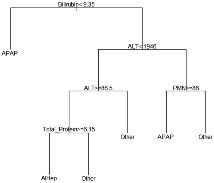
This is a simple example of a CART model. To predict the outcome, one must begin at the top and recursively follow logic statements until a terminal node is reached. For true logic statements, the model follows the left branch, and false logic statements dictate movement to the right branch.

The RF procedure iteratively develops decision trees which can be used in the classification or regression problems. RF is a machine learning algorithm which builds models in multiple steps. First, the dataset is split into two groups: an in-bag (training) set and an out-of-bag (validation) set. The in-bag dataset is used to grow a CART within the forest. A subset of predictor variables is randomly selected and binary splits are made using the best features, as described in the previous paragraph. When the tree is fully grown (i.e. when stopping criteria have been met), the out-of-bag dataset is run down all the trees in the forest. Each decision tree votes for what it predicts for the classification of each observation, and the outcome group with the most votes is the prediction for the model. This process is repeated until the specified number of trees has been created. A detailed discussion of the theory behind the random forest procedure is found in Breiman's seminal paper [4].

There are many reasons that RF is a beneficial statistical tool for classification. Primarily, it does not have the same limitations that inhibit many traditional statistical procedures. For example, the RF procedure can handle the “curse of dimensionality,” when the number of predictor variables is much larger than the sample size. Additionally, RF can be applied when predictors are correlated, provides an unbiased data imputation mechanism, can determine which variables are important in the model, and can capture non-linear patterns between predictors and the outcome of interest [9]. RF differs greatly from its traditional statistical counterparts and offers an alternate method where classical assumptions are not necessary. Thus, the RF method often has much lower prediction error rates than many traditional models, a characteristic which makes it an attractive solution to the problem of classification.

Even though there are many positive aspects to the RF procedure, it does have challenges in implementation and interpretation. The algorithm is quite different from most statistical classification procedures, and many common statistics are not used. RF does not calculate p values, confidence intervals or test statistics in the traditional sense. Moreover, it does not provide users with a closed form of a model due to the complexity of the algorithm, which is partially why random forest is nicknamed the “black box.” Though the procedure lacks many tools that are conventionally used to evaluate models, it is possible to extract similar information from the output. The next section discusses challenges of classification both in general and specifically for the ALF setting.

Challenges of classification procedures

There are many obstacles within the general classification problem which make developing accurate models a challenge. Classification procedures other than RF include logistic regression, linear or quadratic discriminant analysis, principal components and support vector machines [1]. This section focuses on several considerations that are applicable to many of these classification models.

The first challenge to classification of ALF etiologies is the limited number of observations which are drawn in a non-random fashion from the population. A major issue in classifying these patients is that many traditional statistical models for classification are inadequate due to their model assumptions. For example, discriminant analysis and principal components assume multivariate normality of predictor variables drawn from an infinitely large population. Many laboratory variables collected within the ALF registry, such as lipase and ionized calcium, have highly skewed distributions, making the assumption of normality inappropriate. Support vector machines require independent and identically distributed variables, which is violated by ALFSG data since many variables collected are correlated. For instance, alanine aminotransferase (ALT) and aspartate aminotransferase (AST) have a strong positive correlation, and mulitcollinearity would become an issue if both of these variables were included within many statistical classification models.

Another issue is missing data, a problem that is relevant in many disease registries. Furthermore, some sites collect variables regularly that others do not, introducing a non-random missing data pattern for certain variables. Since many statistical classification procedures require complete data, decisions must be made about how to handle missing data. The two main options are to impute missing values or to exclude subjects who have missing values from the analysis. For the data used in this study, some variables have as much as 60% of the observations missing, which is understandable given the large amount of data the registry collects. Withholding patients with missing data from the classification procedures would substantially reduce the sample size, to the extent that employing the procedure would lack generalizability.

In addition to the problem of missing data, there are interesting occurrences within the data which present even more obstacles to accurate classification. Patient variability is extremely high due to the wide variety of ALF etiologies, which range from suicidal drug overdose to pregnancy to viral hepatitis. Procedures such as discriminant analysis and support vector machines are highly sensitive to outliers and noisy data, so these methods may perform poorly for ALF data. Also, ALF is an infrequent illness and some of its etiology categories are rare as well, creating a highly imbalanced dataset. The largest etiology group is acetaminophen overdose, which accounts for about half of ALF cases [3]. Patients from nine of the fifteen total etiology groups represent less than ten percent of all ALF cases in the registry dataset. These rare outcome groups make categorical prediction extremely difficult, regardless of the classification method employed.

There are many obstacles to accurate classification of etiologies in ALF patients. What should seemingly be a straightforward application of a statistical model becomes much more difficult because of these issues. RF was selected as the statistical modeling tool for this setting, offering several solutions to these problems: it can impute missing values, requires few statistical assumptions, and can provide higher prediction accuracy compared to many other classification procedures. The classification problem of ALF etiologies is discussed in detail in the following segment.

Clinical context

The ALFSG began collecting data at more than 15 hospitals across the United States for the registry in 1998 and currently has 16 participating sites. To date, the registry consists of over 2,000 patients who have been affected by ALF. Study data are collected daily seven days following enrollment or until a transplant or hospital discharge occurs, and patients are followed for one year. Information collected includes, but is not limited to, patients' medical history, risk factors and past medications, physical exams including neurological status, imaging, laboratory data, daily updates, vital signs, transplant status and various other clinical characteristics.

The current method for determining a patient's ALF etiology involves extensive and sequential laboratory tests that seek to rule out, or rule in, etiologic categories one at a time. These include detailed historical data regarding medications and possible virus or toxin exposures, routine chemistries including liver function tests, complete blood counts, blood typing, acetaminophen levels, viral hepatitis serologies, tests for Wilson's disease, autoantibodies and pregnancy tests in females [10]. If none of these provide a clear answer, a liver biopsy may be performed. In many cases, the subject is encephalopathic and family may not be available so that this information is not easily gained. After some or all of these tests and surveys are done, the etiology of around fifteen percent of patients remains indeterminate [3]. Thus, the availability of a large, carefully collected registry from many different sites provides a snapshot of the varying etiologies and presentations of ALF across the United States.

The most important decision made by clinicians caring for these patients is whether to list for transplantation. Patients with ALF listed for liver transplantation have a high likelihood of dying within seven days of being placed on the transplant list. The decision to list is of utmost importance since those who undergo transplantation must take immunosuppressive medications indefinitely, while survival without a transplant is typically deemed to be less than 20% for those who are listed for liver transplantation. Avoiding a transplant and dying is not a suitable alternative. Deciding to list a patient for liver transplantation is made after the etiology has been established; hence, this diagnosis is essential for ALF patients. Reducing the amount of time in determining etiology should lead to improved patient outcomes since treatment plans may be implemented after this diagnosis has been established.

To date, little research has investigated the use of RF to predict outcomes in a clinical setting. As with many orphan conditions, researchers are perplexed by the mysteries surrounding ALF. Though the literature for ALF is expanding as more information becomes available, there are still many topics yet to be explored. Lee provides a thorough medical discussion of diagnosing ALF etiologies [3], but there is an immediate need for a statistical model that will supplement these clinical observations in order to improve the accuracy and efficiency of etiology classification.

Application of the RF procedure

The ALFSG collects a multitude of variables related to ALF within the registry. The outcome variable used in the RF is the patients' primary etiology, which falls into exactly one of the total fifteen categories. Figure 2 displays the distribution of etiology for the ALFSG registry as of December 17, 2012. The majority of cases are caused by acetaminophen overdose, which account for 46% of ALF subjects in the database. The next most common groups include indeterminate, drug induced liver failure, hepatitis B, and autoimmune hepatitis, accounting for 12%, 11%, 7% and 7% of the registry data respectively. The ten other categories each comprise less than 5% of all cases in the database, with five of those categories comprising less than 1% of ALF subjects.

Figure 2.

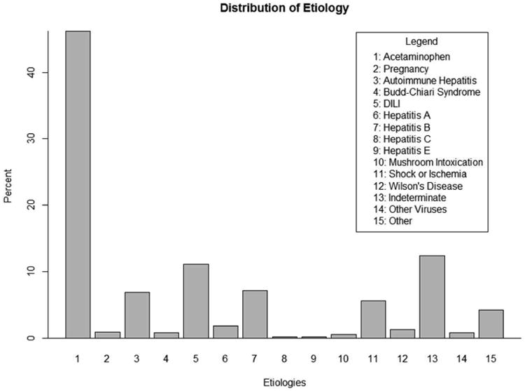
This plot displays the original distribution of the categorical outcome, etiology. There are fifteen total outcome groups, many of which are quite rare. The imbalanced nature of etiology presented a significant challenge to accurate classification.

Due to the sparse structure of the outcome variable in this study, etiologies were grouped based on clinical judgment and data available for each case. New groups consist of: acetaminophen overdose (APAP), drug induced liver injury (DILI), autoimmune hepatitis (AIHep), hepatitis B (HepB), indeterminate (Indeter) and the rest of the etiologies (Other). The distribution of the grouped etiologies is shown in Figure 3. The rarer etiology categories are combined into a larger “other” group make up 16% of the patients. The remaining five categories, unchanged in this grouping, have the same distribution described in Figure 2.

Figure 3.

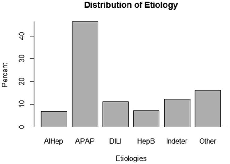
This plot displays the original distribution of the categorical outcome, etiology. There are fifteen total outcome groups, many of which are quite rare. The imbalanced nature of etiology presented a significant challenge to accurate classification.

The RF procedure was employed using this grouped categorization for two main reasons. First, there were extremely high misclassification rates for the rarer categories so that results were not very meaningful using all etiology groups. For the RF applied to all categories, the misclassification rate was close to 100% for several of the uncommon etiology groups. Thus, these groups were combined into one “other” category. Secondly, grouping the etiology categories was sensible from a clinical perspective. Clinicians typically run through several laboratory tests to rule in or out etiology categories when attempting to determine etiology of ALF. Thus, knowing that a patient falls within the “other” group, for example, will at least direct the clinician as to which tests to do first.

For the RF model, researchers considered forty-six explanatory variables which are collected in the ALFSG registry when patients are admitted to the study. There were 1,995 patients in the registry as of December 17, 2012; however, because data imputation techniques require complete data on the outcome variable, only 1,978 of these were included in the dataset for analysis. Exploratory data analysis was performed on the potential explanatory variables for the model. Biologically implausible or impossible values for the continuous variables were removed from the dataset and set to missing. After data were processed in this manner, missing values were imputed using the rfImpute function within the package randomForest in R [11]. The subsequent section discusses results from the RF procedure employed to the ALFSG registry data.

RF results

After data were processed and missing data were imputed, the RF variable selection procedure was implemented using the R package varSelRF, which minimizes the prediction error rate to successively eliminate the least important variables while preserving the overall accuracy and variable importance measures of the RF [12]. Variables selected by the procedure were ALT, amylase, AST, bilirubin, blood urea nitrogen (BUN), ionized calcium, monocytes (monos), lymphocytes (lymph), PMN, phosphate, total protein and number of days from onset until study admission (days from onset).

Using an automated variable selection procedure to determine which variables were most important for the prediction of etiology was beneficial in two main ways. First, researchers wanted to eliminate superfluous variables which were inconsequential for the classification of etiology. Since ALF is an orphan condition, clinical research involving many of the laboratory variables was limited and provided only a few key variables which are known to distinguish etiologies (e.g. ALT and bilirubin). The selection procedure provided a means of understanding which variables were predictive of etiology groups. Another reason for implementing the variable selection procedure was to improve the ease of use for the clinician. If all forty-six variables were included within the final model, clinicians would spend a substantial amount of time gathering and inputting the variables within an application to use the RF. Because a main objective of this study was to improve the efficiency of classifying etiology for ALF patients in practice, it was preferable to minimize the number of required inputs for the RF.

Following determination of variables for the model, the classification of etiology based on these variables was compiled using the randomForest package in R [11]. Before results for the RF with the variables described above are presented, it is worthwhile to discuss the imputation of missing values in the data. As previously mentioned, missing data presented a considerable issue within the data for this classification problem. Figure 4 displays the distribution of missing data for variables selected to be included in the RF model. There are six variables that have between 0 and 20% of its values missing, four variables that have between 20 and 40% of its values missing and two variables that have between 40 and 60% of its values missing. It was decided to include the variables that have substantial amounts of missing data because the RF mechanism for imputation can handle large proportions of missing data [13].

Figure 4.

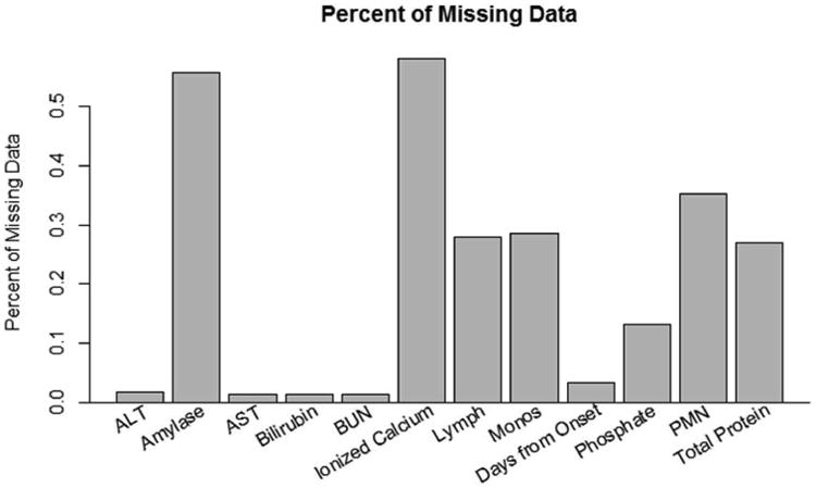
This graph displays the distribution of missing data for independent variables included within the RF after the variable selection procedure. Some variables, such as ionized calcium and amylase, have a substantial proportion of missing data (more than half). However, RF is able to impute missing values even under extreme cases of missing data, such as these variables.

Evaluating Accuracy of the Classification Model

Though it is fairly simple to compile a RF model, it is often not as easy to extract information, either statistics or graphical displays, which can adequately address questions that clinicians have in a manner that they will readily understand. In this setting, clinical personnel may inquire: “If I use this model for a new patient presenting with ALF upon his or her admission to the hospital, what is the probability that an incorrect prediction of etiology will be determined?” The out-of-bag error rate directly answers this question since this is an unbiased measure of cross-validation error for the model. For the ALFSG data used in this study, the out-of-bag error rate was about 35%. This means that if the RF was used to predict the etiology for a new patient, the model would incorrectly classify etiology around 35% of the time. Although this rate seems quite high, given the numerous challenges to classification discussed previously, a 35% error rate for new patients might be the best or one of the best rates that can be achieved based on the data. For the RF containing all forty-six variables initially considered, the out-of-bag error rate was 34%, suggesting that the reduced model performed almost equivalently in terms of overall error of predictions.

Natural follow-up questions that a clinical person may ask are: “Does the model misclassify some etiology categories more often than others?” and “When the model misclassifies patients, which etiology groups does it wrongly predict?” These questions may be addressed numerically using statistics or visually through plots. The confusion matrix and associated class error rates, which are included with basic R output for the RF model, are statistical summaries which investigate misclassification rates by group. Table 1 displays the confusion matrix and class error rates for this study. Columns of the table represent the outcome class that the model predicted for the subjects, and rows represent the actual outcome class of the subject. Thus, the diagonal of the table, shaded in Table 1, represents the numbers of subjects correctly classified by the model. Using this table, information can be gained about which categories contain the incorrect classifications. For example, there were four subjects whose etiology was autoimmune hepatitis, but the model predicted that they would be in the acetaminophen group. Similar interpretations can be made for the rest of the cells in the table.

Table 1.

Predicted Class
Actual Class		AIHep	APAP	DILI	HepB	Indeter	Other	Class Error
	AIHep	63	4	35	5	22	7	0.54
	APAP	1	873	3	2	3	32	0.04
	DILI	29	30	60	17	48	36	0.73
	HepB	7	30	12	48	29	16	0.66
	Indeter	15	49	34	14	87	46	0.64
	Other	10	90	28	12	17	164	0.49

The last column in Table 1 specifies the error rate of the model, broken down by outcome categories. For this model, the rate of misclassification was very low for the acetaminophen etiology group, was moderate for the autoimmune hepatitis and other groups, and was fairly high for the remaining groups. There are substantial differences between class error rates because the default settings in the randomForest R package seek to minimize the out-of-bag error rate. If it is more important that certain outcome groups are accurately predicted, weights may be applied to the model to increase or decrease the error rates of specific classes. Of course, decreasing the class error rate of one group may cause the other outcome groups' error rates to increase, as well as the overall out-of-bag error rate. For the prediction of etiology, class weights were not applied to the model because the cost of incorrect classification for each group was the same from a clinical standpoint in this study. Compared to the RF containing all forty-six variables, the class error rates for the model containing the twelve selected variables were quite similar. The largest difference was in the error rate for the Other group, which was 49% for the reduced model and 53% for the full model. The remaining etiologies differed less than 1%, suggesting that both models performed similarly regarding class error rates.

The confusion matrix in Table 1, along with the class error rates for the model, can be overwhelming and it may be difficult to deduce a clear summary of model misclassification by group. A visual method for presenting the same results can be produced using a measure called the margin. The margin of a data point is the proportion of votes for the correct class minus the maximum proportion of votes for the remaining classes. Thus, positive margins correspond to correct prediction and negative margins mean incorrect prediction [11]. Moreover, the margin of an observation serves as a measure of confidence in correct classification. They are contained in the interval [-1, 1]; margins closer to 1 indicate higher confidence in accurate classification and margins closer to -1 indicate lower confidence in accurate classification [14].

Figure 5 shows two graphical representations of the margins for the classification of etiology. The histogram of the margins is skewed left, indicating that the majority of observations were correctly classified for the data in aggregate. The side-by-side boxplots of the margins by diagnosis category allow visualization of the accuracy of prediction for each group. The acetaminophen group's boxplot lies mostly in the positive range, meaning that the RF model predicts correctly for the majority of subjects in this category. The medians of the boxplots for the autoimmune hepatitis and other groups are around zero, indicating that the model correctly predicts these outcomes for half of the patients within these groups. However, the boxplots for the drug induced liver injury, hepatitis B and indeterminate groups all have medians less than zero, which represents misclassification of more than half of these subjects. This information is consistent with the class error rates and confusion matrix displayed in Table 1.

Figure 5.

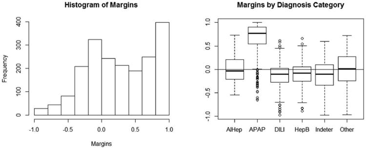
The histogram of margins (left) is right-skewed, indicating that the correct etiology for the majority of patients was determined by the RF. The box plots (right) visualize margins by etiology groups, illustrating that the RF predicts with high confidence for APAP, moderate confidence for AIHep, and lower confidence for the remaining groups.

Analyzing Variables within the Model

Aside from evaluating the accuracy of the RF as a whole and broken down by outcome groups, there is interest in gaining information about which variables are actually influencing the prediction model. To assess which variables are important within the RF, two measures can be considered: the mean decrease in accuracy and the mean decrease Gini [9]. The latter is based on the number of splits within the decision trees for each predictor, and is criticized for its bias for continuous variables. Because continuous variables have many more options for where splits can occur within each decision tree in the random forest, the mean decrease Gini tends to give higher importance to these variables, as opposed to ordinal or categorical variables which have a limited number of places for splits to occur. Another importance measure is the mean decrease in accuracy, which is the difference between the out-of-bag error rate from a randomly permuted dataset and the out-of-bag error rate of the original dataset, expressed as an average percent over all trees in the forest. For both of these importance measures, high values represent important variables and low values represent unimportant variables in the RF framework.

In the plots in Figure 6, the variables are ordered from most important at the top to least important at the bottom. The two criteria for evaluation of importance disagree slightly, but it is evident that some variables are more valuable in predicting etiology than others. The top five important variables for the classification of etiology in ALF patients are bilirubin, number of days from onset to study admission (Days from Onset), ionized calcium, ALT and monocytes (Monos). The most important variables differ by criterion; however, this is not surprising since they are calculated based on different measures. The variable importance plot for the RF containing all forty-six input variables identified the twelve variables chosen by the selection procedure as the most important, while maintaining almost the exact order. This again indicated minimal presence of bias for the reduced model containing only twelve variables.

Figure 6.

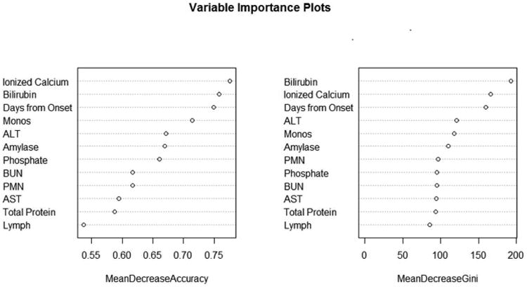
Plots for variable importance measures are presented. Though the exact ordering is different for mean decrease in accuracy and mean decrease in Gini, the top three most important variables in predicting etiology are bilirubin, days from onset, and ionized calcium.

While it is helpful to learn about which variables are important in the model overall, clinicians may additionally wonder if certain variables are more important for some etiology categories than others. Since there is such a wide range of etiologies, it is highly plausible that this is the case. An inquiry along these lines may be, “How important is bilirubin in predicting that a patient's acute liver failure was caused from hepatitis B?” A statistical measure gathered from the RF called local importance may be used to answer this question. The local importance of a variable for each prediction is defined as the percent of votes for the correct class in the out-of-bag data less the percent of votes for the correct class in the permuted out-of-bag data. Positive values of local importance indicate that the variable aids in correct prediction and negative values indicate poor impact on correct prediction.

Boxplots of the local importance for each observation are displayed in Figure 7 for the four most important variables according to the mean decrease in accuracy criterion. These are helpful in seeing differences between etiology groups. From the boxplot of local importance for bilirubin, one deduces that bilirubin has a strong positive impact in predicting that a patient's liver failure was caused by hepatitis B because the boxplot lies entirely above zero. Similar interpretations can be made for the classification of autoimmune hepatitis, indeterminate and drug induced liver injury. The medians and first quartiles for each groups' boxplots of local importance are all positive, indicating that bilirubin does positively impact correct classification for the majority of observations. This is consistent with the results presented in the variable importance plots in Figure 6. Analogous interpretations can be inferred in analyzing the three other plots. Recall that a variable selection procedure was used to determine the most important variables for inclusion in the RF. For this reason, the local importance plots indicate that each variable is important in the prediction of etiology. If a variable selection procedure had been omitted, it is likely that the local importance plots would distinguish essential and nonessential variables for the prediction of etiology.

Figure 7.

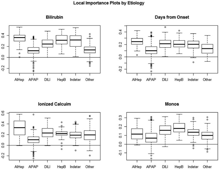
Local importance plots by etiology groups are presented for four variables: bilirubin, days from onset, ionized calcium, and monocytes. These allow for distinguishing which variables are more or less important in determining specific etiologies.

For continuous predictors, partial dependence plots may be constructed to further analyze the probability of classification in each group. The boxplots of margins are useful in understanding which variables are important for specific outcome categories, but partial dependence plots allow for conclusions about the relationship between continuous predictor variables and the likelihood the model will classify subjects to specific groups. For example, a clinician may ask, “As the value of ionized calcium increases, how does the probability that a patient is determined to have ALF caused by autoimmune hepatitis change?” These plots visualize the probability of an etiology group for values of a predictor variable when the effects are averaged over all other features. The horizontal axis is the predictor variable in its original units and the vertical axis values are related to the log odds of realizing each outcome class. Hastie et al. gives a detailed description and derivation of partial dependence plots for the random forest model [1]. To summarize, positive slopes within partial dependence plots represent higher probabilities of being classified within the outcome group and negative slopes are associated with lower probabilities of being classified within the outcome group.

The partial dependence plot for ionized calcium is found in Figure 8. To analyze the association between ionized calcium and the probability of being included in a specific etiology group, one must trace the slope of the line. The slope of the autoimmune hepatitis group is positive until around 2 mg/dL and levels off after that. This means that as ionized calcium increases up to 2 mg/dL, the probability of a patient being classified in the autoimmune hepatitis etiology group increases. For values of ionized calcium greater than 2 mg/dL, the chance of being classified in autoimmune hepatitis remains the same. This interpretation holds while all other variables included in the model are fixed. Conclusions along these lines may be deduced from the relationship between the slope and the other etiology groups as well. Partial dependence plots, such as the one shown in Figure 8, may be constructed for any continuous variables included in the RF model.

Figure 8.

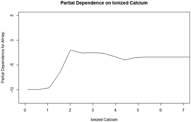
The partial dependence plot on ionized calcium for the autoimmune hepatitis outcome group is presented. The slope of this plot indicates that as ionized calcium increases to 2 mg/dL, the probability the ALF was caused by autoimmune hepatitis increases, while other variables remain constant. Values above 2 mg/dL are associated with constant probabilities ALF was caused by autoimmune hepatitis since the slope of the plot levels off.

Subject-specific Information

Although information about which variables are important in the model can be useful in analyzing the relationships between predictors and the outcome of interest, clinicians are often interested in more detailed information for their specific patient. A common question may be, “What is the probability that my patient will be classified into each etiology group based on the information I have?” To address this question, the probabilities of classification in each group may be extracted from RF output. Since each tree votes for which category it predicts for an individual patient, the probability of inclusion for outcome groups may be calculated by dividing the number of votes for each group by the number of trees in the forest.

Thus, if the prediction for the model is incorrect, a classification for the next most likely groups can be determined. The RF model correctly determines the classification of etiology with 65% accuracy for its first prediction, and correctly determines the etiology with 80% accuracy for its first or second prediction. Allowing the model to predict two categories, there is a marked increase in the predictive power of the model. This is extremely helpful for the diagnosis of ALF etiologies because of the way that clinicians run many tests in order to determine the etiology of a patient. Subsequently, if the model makes an incorrect prediction the first time, it provides clinicians an idea for the next test to run. Given the highly variable patient population, having access to the probability that the etiology of a patient will fall into each group creates a road map for the sequence of tests that doctors complete in determining the cause of ALF. As a result, the method for diagnosing liver failure for each affected patient can be more efficient and accurate based on information gained from RF results.

Discussion

The main purpose of this paper was to investigate the use of the RF procedure for classification in a clinical setting and provide guidance on the interpretation of the procedure results. This paper contributes to the current literature related to the application and interpretation of the RF model, providing an in-depth discussion of specific clinical questions and suggested output and graphical displays. RF offers an effective and generalizable statistical framework that can be used in many different circumstances: classification, continuous prediction, survival analysis, and unsupervised learning (clustering). Improved understanding of how the algorithm functions and how the results can be interpreted to answer clinical questions is essential to increasing its use.

Though this study offers insight into the use of RF in a clinical setting, there are limitations that should be considered. First, the issue of introducing bias into the model through missing data should be mentioned. All of these analyses only hold with the caveat that the model may be influenced by biased imputed data. Since all data, including both test and training data, are used to impute missing values, bias may be introduced. However, this problem would be present with any dataset containing imputed values, and imputation is a much more attractive alternative than only including patients who have complete data in the analysis.

A potential drawback of using a variable selection procedure is the possibility of biased results because the varSelRF procedure uses both the training and test datasets. However, bias appeared to be minimal in this study, as presented in the results: the out-of-bag error, class error rates, and order of variable importance were similar for both the RF containing all predictors and the RF containing only the twelve predictors selected. Thus, the use of a model containing the twelve variables selected was preferable for predicting etiology because bias was limited and efficiency of model use for clinicians was markedly increased. Though for this study bias was likely minimal, it is recommended to assess the impact of variable selection procedures on RF performance, using a model containing all covariates as a benchmark.

Another limitation to this study is that the RF procedure does not output traditional statistical measures such as p values and test statistics. Though alternatives to these statistics are plentiful, presenting a completely different framework for analysis may be challenging. For example, the algorithm provides two measures of variable importance which may favor or disfavor predictors depending on the scale of the measurement or the number of groups for categorical variables. Importance measures are also criticized because they are sensitive to the number of trees in the forest and the number of predictor variables selected, both of which are parameters that the user defines. Furthermore, variable importance is not necessarily synonymous with statistical significance. Variables may be important in the RF but may not be statistically or clinically significant. Some researchers have proposed ways for testing statistical significance of variables within the RF framework, but currently there is not a straightforward, universally accepted method for employing these tests [15, 16].

Specific to the ALF clinical setting, conclusions from this study should result in more accurate and efficient diagnosis of the cause of ALF. It is critical for correct classification of the cause of ALF so that clinical personnel may develop an appropriate treatment plan for patients and decide if patients should be placed on the transplant waiting list. Also, results from this paper supplement current knowledge about the relationships between variables collected within the registry and etiology groups. Many of the patterns extracted from the RF procedure are consistent with the clinical literature currently available, and some provide new variables for clinicians to consider in the determination of etiology. Information generated from this study provides a much needed supplement to clinicians attempting to diagnose the etiology of liver failure in affected patients.

There are several additional avenues of future research within this topic. RF is still a fledgling statistical procedure, and improvements are needed in terms of application and analysis. A more standardized method for presenting and interpreting results should be established so that researchers can easily deduce conclusions. For example, a test to determine which variables are statistically significant in the model would provide a clearer picture of the relationship between predictors and the outcome classification. Additionally, measures of uncertainty or confidence intervals would be helpful in reporting statistics such as local importance and partial dependence.

References

- 1.Hastie T, Tibshirani R, Friedman J. The elements of statistical learning. 2nd. Springer; New York: 2001. [Google Scholar]
- 2.Hoofnagle J, Carithers R, Sapiro C, et al. Fulminant hepatic failure: summary of a workshop. Hepatology. 1995;21:240–252. [PubMed] [Google Scholar]
- 3.Lee WM. Etiologies of acute liver failure. Seminars in Liver Disease. 2008;28:142–152. doi: 10.1055/s-2008-1073114. [DOI] [PubMed] [Google Scholar]
- 4.Breiman L. Random forests. Machine Learning. 2001;45:5–32. [Google Scholar]
- 5.Díaz-Uriarte R, De Andres SA. Gene selection and classification of microarray data using random forest. BMC bioinformatics. 2006;7 doi: 10.1186/1471-2105-7-3. [DOI] [PMC free article] [PubMed] [Google Scholar]
- 6.Cutler DR, Edwards TCJ, Beard KH, et al. Random forest for classification in ecology. Ecology. 2007;88:2783–2792. doi: 10.1890/07-0539.1. [DOI] [PubMed] [Google Scholar]
- 7.Larivière B, Van den Poel D. Predicting customer retention and profitability by using random forests and regression forests techniques. Expert Systems with Applications. 2005;29:472–484. [Google Scholar]
- 8.Breiman L, Friedman JH, Olshen RA, Stone CJ. Classification and regression trees. Wadsworth and Brooks; Monterrey, CA, USA: 1984. [Google Scholar]
- 9.Boulesteix AL, Janitza S, Kruppa J, et al. Overview of random forest methodology and practical guidance with emphasis on computational biology and bioinformatics. Wiley Interdisciplinary Reviews: Data Mining and Knowledge Discovery. 2012;2:493–507. [Google Scholar]
- 10.Polson J, L WM. AASLD position paper: the management of acute liver failure. Hepatology. 2005;41:1179–1197. doi: 10.1002/hep.20703. [DOI] [PubMed] [Google Scholar]
- 11.Liaw A, Weiner M. Classification and Regression by randomForest. R News. 2002;2:18–22. [Google Scholar]
- 12.Diaz-Uriarte R. Package ‘varSelRF’. The R Project for Statistical Computing. 2013 [Google Scholar]
- 13.Breiman L, Cutler A. Random forests. Random forests. 2007 web page. [Google Scholar]
- 14.Schapire RE, Freund Y, Bartlett P, et al. Boosting the margin: a new explanation for the effectiveness of voting methods. The Annals of Statistics. 1998;26:1651–1686. [Google Scholar]
- 15.Altmann A, Tolosi L, Sander O, et al. Permutation importance: a corrected feature importance measure. Bioinformatics. 2010;26:1340–1347. doi: 10.1093/bioinformatics/btq134. [DOI] [PubMed] [Google Scholar]
- 16.Wang M, Chen X, Zhang H. Maximal conditional chi-square importance in random forests. Bioinformatics. 2010;26:831–837. doi: 10.1093/bioinformatics/btq038. [DOI] [PMC free article] [PubMed] [Google Scholar]