Dissecting the Phenotypic Components of Crop Plant Growth and Drought Responses Based on High-Throughput Image Analysis^,

A framework for high-throughput analysis of phenotypic traits from nondestructive plant imaging is used to dissect phenotypic components of barley growth and crop performance.

Abstract

Significantly improved crop varieties are urgently needed to feed the rapidly growing human population under changing climates. While genome sequence information and excellent genomic tools are in place for major crop species, the systematic quantification of phenotypic traits or components thereof in a high-throughput fashion remains an enormous challenge. In order to help bridge the genotype to phenotype gap, we developed a comprehensive framework for high-throughput phenotype data analysis in plants, which enables the extraction of an extensive list of phenotypic traits from nondestructive plant imaging over time. As a proof of concept, we investigated the phenotypic components of the drought responses of 18 different barley (Hordeum vulgare) cultivars during vegetative growth. We analyzed dynamic properties of trait expression over growth time based on 54 representative phenotypic features. The data are highly valuable to understand plant development and to further quantify growth and crop performance features. We tested various growth models to predict plant biomass accumulation and identified several relevant parameters that support biological interpretation of plant growth and stress tolerance. These image-based traits and model-derived parameters are promising for subsequent genetic mapping to uncover the genetic basis of complex agronomic traits. Taken together, we anticipate that the analytical framework and analysis results presented here will be useful to advance our views of phenotypic trait components underlying plant development and their responses to environmental cues.

INTRODUCTION

A central goal of biology today is to map genotype to phenotype. High-throughput genotyping platforms support the discovery and analysis of genome-wide genetic markers (genotypes) in populations in a routine manner (Davey et al., 2011; Edwards et al., 2013). However, our capabilities for systematic assessment and quantification of plant phenotypes have not kept pace (Houle et al., 2010; Furbank and Tester, 2011). Commonly used conventional phenotyping procedures are labor-intensive, time-consuming, lower throughput, costly, and frequently destructive to plants (e.g., fresh or dry weight determination), whereas measurements are often taken at certain times or at particular developmental stages, a scenario known as the “phenotyping bottleneck” (Furbank and Tester, 2011).

Recently, the introduction of techniques for high-throughput phenotyping has boosted the area of plant phenomics, where new technologies such as noninvasive imaging, spectroscopy, robotics, and high-performance computing are combined to capture multiple phenotypic values at high resolution, high precision, and in high throughput. This will ultimately enable plant scientists and breeders to conduct numerous phenotypic experiments in an automated format for large plant populations under different environments to monitor nondestructively the performance of plants over time (Eberius and Lima-Guerra, 2009). Various automated or semiautomated high-throughput plant phenotyping platforms have been developed recently and are applied to investigate plant performance under different environments (Granier et al., 2006; Walter et al., 2007; Biskup et al., 2009; Jansen et al., 2009; Arvidsson et al., 2011; Golzarian et al., 2011; Nagel et al., 2012). The huge amounts of image data routinely accumulated in these platforms need to be efficiently managed, processed, and finally mined and analyzed. Thus, we are now facing the “big data problems” (Schadt et al., 2010) brought about by such real-time imaging technologies in the phenomics era. Although several analytical tools (Bylesjö et al., 2008; Weight et al., 2008; Wang et al., 2009; Hartmann et al., 2011; Green et al., 2012; Karaletsos et al., 2012) provide general image-processing solutions for extracting a wide range of plant morphological measurements (such as plant height, length and width, shape, projected area, and digital volume) and colorimetric analysis, they are individually designed to address specific questions (Sozzani and Benfey, 2011). The trait information gained from these tools is still very limited. Furthermore, the phenotypic components underlying dynamic processes in plants such as growth, development, or responses to environmental challenges and their properties remain unexplored. For these reasons, there is increasing demand for software tools that are capable of efficiently analyzing large image data sets and subsequent statistical methods to investigate comprehensively collected phenotypic data.

Automated noninvasive precise high-throughput phenotyping is especially interesting in the context of dissecting the complex genetic architecture of biomass development and of drought stress tolerance. Impact of drought depends heavily on timing and intensity of the dry period and on environmental conditions (Calderini et al., 2001; Araus et al., 2002) hampering heritability as a prerequisite for genetic mapping of quantitative trait loci (QTL) (Ribaut et al., 1997; Painawadee et al., 2009; Sellammal et al., 2014). Drought tolerance has been investigated in various QTL studies since the start of the molecular marker age (Lilley et al., 1996; Xiong et al., 2006; Szira et al., 2008; Nezhad et al., 2012). Adequate controlled phenotyping and daily phenotypic observation of drought stress development has a huge potential to boost the understanding of the genetics of drought tolerance.

Here, we present a powerful solution that was developed alongside currently available high-throughput image data processing pipelines, such as our Integrated Analysis Platform (IAP) (Klukas et al., 2014). We implemented various algorithms for efficient analysis and interpretation of huge and high-dimensional phenotypic data sets to support understanding plant growth and performance. We applied our pipeline to a core set of 18 different barley (Hordeum vulgare) cultivars, which were daily imaged under well-watered and drought stress conditions. We extracted and quantified a list of representative phenotypic traits from the digital imaging data. We used linear mixed models to dissect variance components of phenotypic traits and showed that the traits revealed variable genotypic and environmental effects and their interactions over time. Key parameters such as trait heritability and genetic trait correlations were assessed, indicating image-derived traits are valuable in genetic association studies. Finally, we used several linear and nonlinear functions to model biomass accumulation for both control and stressed plants that allow biological interpretation of parameters. Model-derived parameters revealed several important aspects regarding plant development and provide a solid basis for subsequent QTL analysis aimed at understanding the genetic control of plant growth.

RESULTS

Extraction of Phenotypic Traits from High-Throughput Image Data

We applied our methodology to a compendium of ∼50,400 images (∼100 GB of data) collected for 18 barley genotypes from four agronomic groups (Table 1), with six (for double haploid [DH] lines) or nine (for non-DH lines) replicated plants per genotype per treatment. Over a course of 7 weeks, plants were monitored in a noninvasive way under control and drought stress conditions using an automated plant transport and imaging system (Figures 1 and 2; see Methods). Three types of image data, near-infrared (NIR), visible (color), and fluorescence (FLUO) images, were acquired daily from different views (top view and side views from different angles) in the phenotyping system. For example, color imaging can be used to assess growth status and biomass accumulation of plants as well as their nutritional or health status, while NIR imaging provides a measure related to plant water content and FLUO imaging detects signals of chlorophyll and other fluorophores (Berger et al., 2010). Data retrieved from the imaging platform were organized into our IAP system (Klukas et al., 2014) and processed through an analysis pipeline specifically adjusted for mid-sized important crop species such as barley, resulting in values of nearly 400 phenotypic traits extracted from images of each individual plant (Figures 2A and 2C).

Table 1. Overview of 18 Barley Genotypes Used in This Study.

Agronomic Group	Genotypea	Release	Breeder	Pedigree
DH	BarkeDH	1996	Breun	Libelle x Alexis
DH	MorexDH	1978	MN AES	Cree x Bonanza
1	Ackermanns Bavaria	1910	Ackermann	Selection from Bavarian landrace
1	Heils Franken	1895	Heil	Selection from Franconian landrace
1	Isaria	1924	Ackermann	Danubia x Bavaria
1	Pflugs Intensiv	1921	Pflug	Selection from Bavarian landrace
2	Apex	1983	Lochow	Aramir x (Ceb.6721 x Julia x Volla x L100)
2	Perun	1988	Hrubcice/NKGNord	HE 1728 x Karat
2	Sissy	1990	Streng	(Frankengold x Mona) x Trumpf
2	Trumpf (Triumpf)	1973	Hadmersleben	Diamant x 14029/64/6 ((Alsa x S3170/Abyss) x 11719/59) x Union
3	Barke	1996	Breun	Libelle x Alexis
3	Beatrix	2004	Nordsaat	Viskosa x Pasadena
3	Djamila	2003	Nordsaat	(Annabell x Si 4) x Thuringia
3	Eunova	2000	Probstdorf	H 53 D x CF 79
3	Streif	2007	Saatzucht Streng GmbH & Co. KG	Pasadena x Aspen
3	Ursa	2001	Nordsaat	(Thuringia x Hanka) x Annabell
3	Victoriana	2007	Probstdorfer Saatzucht	(LP 1008.5.98 x LP 5191) x Saloon
3	Wiebke	2000	Nordsaat	Unknown

The double haploid population parents are indicated with “DH.” Cultivar Morex is a six-rowed, spring barley from the US. All other cultivars are two-rowed spring barleys released in Germany. Genotypes are grouped according to the year of release (except for DH lines).

^aBold indicates the short name used in all the figures.

Figure 1.

Experimental Design.

(A) The growth stages of spring barley.

(B) High-throughput phenotyping of barley plants in a LemnaTec system (http://www.lemnatec.com/).

(C) Plants were monitored in a noninvasive way under control and drought stress conditions. Drought stress (in dash box) was treated at the stage of “stem extension” as indicated in (A).

Figure 2.

Pipeline for Analysis of High-Throughput Phenotyping Data in Barley.

(A) The workflow used for barley phenotyping data analysis. High-throughput imaging data from the LemnaTec system were imported and processed using the barley analysis pipeline in the IAP system. The extracted phenotypic traits were further processed and evaluated (see Methods).

(B) Input (left) and result (right) images in the analysis pipeline. Shown are images from 44-d-old plants (the last day of stress phase) captured by VIS, FLUO, and NIR cameras from the side view.

(C) Classification of phenotypic traits. Traits are classified into four categories: color-related, NIR-related, FLUO-related, and geometric features, based on images obtained from three types of cameras and two views.

(D) Phenotypic traits revealing the stress symptom. Left: An example shows a NIR-related trait over time. Right: heat map shows NIR intensity difference, measured by the ratio value between control and stress plants. Blue indicates low difference, whereas red indicates high difference. Note that plants from different genotypes show different patterns, indicating their different stress tolerance.

These phenotypic measurements can be classified broadly into four categories: plant geometric traits (measuring shape descriptors of plants), color-related properties, NIR signals, and FLUO-based traits (Figure 2C). Quantitative traits were first evaluated based on their reproducibility among replicated plants (see Methods; Supplemental Figures 1A and 1B) against random plant pairs to avoid introducing low quality or weak phenotypic traits into the analysis. A total of 173 (44.6%) traits showed high reproducibility among replicate samples after removing outliers (Pearson correlation coefficient r > 0.8 and one-sided Welch’s t test P < 0.001; Figure 2A). We found that 87.0% of traits that showed genotypic effects or 93.1% of traits that showed treatment effects (adjusted P < 0.01; see below) passed this filtering (Supplemental Figure 2), indicating that we still covered most of the informative traits though the stringent applied criteria. Clustering analysis of these highly reproducible traits showed that large sets of traits were excessively correlated with each other (Supplemental Figure 3), indicating that these traits might be highly redundant descriptors of plant properties within our investigated cultivar set. To get an optimal set of phenotypic traits for a statistical model, we applied the indicator of variance inflation factors (O'Brien, 2007) (variance inflation factor > 5) to remove redundant and noninformative features (see Methods). After manual checking, we selected 54 (31.2%) traits from the entire set of reproducible measures and used them in the remaining analysis (Figure 2A; Supplemental Figure 1C and Supplemental Table 1). However, we note that this barley collection is relatively small, and some of the excluded phenotypic traits might be considered when applying the model to larger plant populations.

Image-Derived Parameters Reflect Drought Stress Responses

Many of the phenotypic changes (such as changes of biomass) were readily detectable upon stress treatment, whereas others (such as dynamics of water content) were less obvious or too subtle to be discerned by eye (Figure 2B; Supplemental Figure 4). Previous studies have suggested that plant water stress might be monitored effectively using NIR imaging (Knipling, 1970; Tucker, 1980; Berger et al., 2010; Munns et al., 2010). We showed that the highly reproducible NIR intensity trait is an effective feature for monitoring plant responses to drought (Figure 2D; Supplemental Figure 1C). Plants showed a rapid decrease of the NIR signal after about 6 d of drought stress. Restoration of the NIR signal was seen after rewatering. The NIR-based indicator also provides a measure of the different abilities to recover among different genotypes (Figure 2D).

To explore more comprehensively the ability of these traits to reflect the responses to the external treatment, we adopted a support vector machine (SVM)-based approach (Loo et al., 2007; Iyer-Pascuzzi et al., 2010), in which “optimal” hyperplanes separate treated and untreated samples (Supplemental Figure 5A). We found that accuracy in distinguishing between stressed and control plants reached over 90% after 1 week of drought stress and nearly 100% separability after 10 d of stress (Supplemental Figure 5B). Besides, the “phenotypic direction” (the normal vector of the hyperplane in SVM) of greatest separation between the two groups of plants revealed three grouped patterns over time, corresponding to the three different treatment periods: growth before onset of drought treatment, during drought stress, and in the recovery phases (Supplemental Figure 5C). These results suggest that the treatment effects of these traits changed dynamically according to the external treatment and growth stage (see below).

Plant Phenomic Map and Phenotypic Similarity

To gain a global plant phenotypic map across the entire cultivar set, clustering approaches were performed on the comprehensive phenome-wide data (Figures 3A and 3B). This map provides important information regarding plant phenotypic similarity or dissimilarity and supports further evaluation of the defined traits. From a cluster analysis with complete linkage applied to the normalized data set, we found that stressed plants were clearly distinguished from control plants irrespective of genotype, but plants of the same genotype or among agronomic groups tended to be grouped together (Figure 3A, upper panel), supporting the idea that similar genotypes lead to similar phenotypes. For the 54 investigated traits, correlation coefficients of trait profiles between pairs of genotypes of the same agronomic groups were significantly higher than pairs of different groups (P < 2.2 × 10⁻¹⁶, one-sided Mann-Whitney U-test; Figure 3A, lower panel). Similar results were observed in a large genome-wide association study mapping population, in which 34 traits were investigated across 413 diverse rice (Oryza sativa) accessions in the field (Zhao et al., 2011). To fine visualize phenotypic similarity revealed by genotype similarity, we performed a self-organizing map (Kohonen, 1990) clustering analysis on the data set (Figure 3B). The self-organizing map plot showed that plants from the same genotype were concentrated at certain locations in the map, and stressed plants were clearly separated from the control plants.

Figure 3.

Phenotypic Similarity Revealed by Genotype Similarity.

(A) and (B) Clustering analysis of phenomic profiling data. HCA (A) and a six-by-six self-organizing map (SOM) (B) were used to reveal the phenotypic similarity of all the investigated barley plants based on the highly reproducible traits. In (A), colored bars along the top of the heat map reflect the sampled agronomic group assignment (groups 1 to 3 and DH) as labeled. Colored bars along the left indicated the corresponding genotypes of individuals as listed in the key. The lower panel shows the median correlation values among individual plants from the same agronomic groups and different groups. In (B), plants with similar genotypes or treatments tend to be at nearby map locations. Control and stress plants are colored and indicated in blank and filled points, respectively. The numbers in the key show the number of plants from the same genotypes belonging to the control or stress group.

(C) Phenotypic similarity trees showing the phenotypic relationship of plants from agronomic groups 1 to 3 under control (left; blank shapes) and stress (right; filled shapes) conditions. The trees were constructed from overall phenotypic distance matrices (see Methods).

(D) Scatterplot indicating the degree of correlation of phenotypic distance between genotypes under both control (x axis) and stress conditions (y axis). Mantel test was performed to examine whether the phenotypic distances in the two conditions correlate with each other. P value was calculated with Monte-Carlo simulation (with 10,000 permutations). Genotype pairs that are far away from the regressed line (red) are labeled and colored (orange, small distances in control and large distances in stress; blue, otherwise).

We next deduced a neighbor-joining tree (termed “phenotypic similarity tree”) based on the 54 informative traits to reveal the phenotypic similarity of plants of different origins (see Methods). We constructed the phenotypic similarity trees for plants cultivated under control and stress conditions, respectively (Figure 3C). We observed that members of the same agronomic groups belonged to closed branches of the tree (Figure 3C, left), reflecting the domestication and breeding history of these cultivars. The phenotypic similarity tree reshaped following the drought stress, although the relative relationship of most cultivars within the same groups was unchanged (Figure 3C, right). Consistent with this observation, the phenotypic distance matrices of these two trees are positively associated (Pearson’s coefficient r = 0.71 and P < 0.001, Mantel test; Figure 3D). However, we observed that barley cultivars such as Apex, Djamilia, and Heils Franken showed least robustness in maintaining their phenotypic relationship when they were exposed to drought stress (Figures 3C and 3D), suggesting that the phenotypic plasticity of these cultivars in response to stress treatment is different.

Phenotypic Profile Reflects Global Population Structure

To further explore the phenotypic relationships of these plants, we performed principal component analyses (PCA) to capture global phenotypic variation in the whole population and to extract specific phenotypic traits relevant for the discrimination of agronomic groups (Figure 4; Supplemental Figure 6). The top six principal components (PCs) explain at least 60% of the total phenotypic variation (Figure 4A). Notably, the accumulative variance explained by these PCs increases with plant growth, having a slight peak at the end of stress phase, accounting for 83.3% of total variation. The increasing accumulative variance over time was observed for control and stressed plants, respectively (Supplemental Figures 7A and 7B), indicating that plants showed more phenotypic differences at the later growth stage.

Figure 4.

Phenotypic Profile Reflects Global Population Structures in the Temporal Scale.

(A) Projections of top six PCs based on PCA of phenotypic variance over time. The percentage of total explained variance is shown. The stress period is indicated by the dashed box.

(B) Scatterplots showing the PCA results on DAS 44 (explained the largest variance). The first six PCs display 83.3% of the total phenotypic variance. The component scores (shown in points) are colored and shaped according to the agronomic groups (as legend listed in the box). The component loading vectors (represented in lines) of each variable (traits as colored according to their categories) were superimposed proportionally to their contribution. See also Supplemental Figures 6 and 7.

At the end of the stress period, the first PC (PC1) explains more than half (52.9%) of the phenotypic variation, which perfectly separated stressed plants from control plants (Figure 4B). Accordingly, geometric and NIR intensity traits are the main factors in the trait space separating these two groups of plants. Meanwhile, PC1 gradually increases along the stress phase, while it decreases when plants recovered with watering, suggesting that more phenotypic variance can be observed between control and stressed plants under more serious stress. Other PCs with smaller proportions of explained variance generally distinguish plants of different agronomic groups from each other. For example, PC2 was mainly driven by the phenotypic difference in groups 2 (released before 1990) and 3 (released after 1990) (Figure 4B), corresponding to the main PCs as observed in control (Supplemental Figure 7C) and stressed plants (Supplemental Figure 7D). Interestingly, more diversity in color-related traits was observed in plants of agronomic group 2, likely revealing the human selection of breeding of these cultivars. The third principal component (PC3) mainly distinguishes plants of agronomic group 1 from the DH group (Figure 4B; Supplemental Figures 7C and 7D). However, the different patterns in the PCA from control and stress plants (Supplemental Figures 7A and 7B) can be explained in part by complex genotype-treatment interactions. Overall, the observations that the first PC separates control and stress plants and that the other PCs separate agronomic and genotype groups are in agreement with the results of the clustering analysis, which showed that plants had larger phenotypic dissimilarity between treatments than between genotype groups (Figure 3A), further indicating that the environment (drought stress treatment) shows dramatic effects on plant growth and development.

Dynamic Genotypic and Environmental Effects on Phenotypic Variation

We used a linear mixed model to decompose phenotypic variance (P) into different causal agents: genetic (G) and environmental (E) sources, and their interaction effects (G×E). The mixed-effects model was fitted using a restricted maximum likelihood approach, and the statistical significance of variance components was estimated by the log-likelihood ratio test (log-LR test; see Methods). We found temporal dynamics of genotypic and environmental influences on overall trait development (Figures 5A and 5B). In the early growth phase, phenotypic variance was mostly the result of unknown environmental effects (residual effects). As plants grew, genotypic factors became more important. The increasing genetic effect on phenotypic variance was observed up to about 6 d after the onset of stress treatment, after which the environmental factors (e.g., drought stress) became progressively more important, while the genetic effect became relatively less important. Although less obvious, the opposite pattern was seen in the recovery phase (Figure 5A), likely due to the decline in phenotypic differences between control and stressed plants. The decline in error variance and increase in environmental variance are reflected by a dynamic change of the total experimental coefficient of variation (CV) over time based on the investigation of geometric traits (Figure 5B). The total experimental CV increased as the drought stress became more severe and declined during the recovery phase. However, the genetic CV across the cultivars was relatively constant upon drought treatment. The genetic CV in stressed plants became less than that in control plants after the onset of treatment (Figure 5B), indicating that plants showed more phenotypical diversity under normal growth conditions than in stressed conditions. Genetic CV peaked at the beginning of plant growth, revealing heterogeneity of plant growth at the initial growth stage. We also observed a moderate level of G×E interaction effects (with the proportion of explained phenotypic variance ranging from 2.6 to ∼15.4%; Figure 5A), indicating that there are genetic differences in the response to drought among different cultivars. We found that the G×E effects progressively increased with plant development, independent from external environment changes.

Figure 5.

Dissection of the Sources of Phenotypic Variance.

(A) Dissecting the phenotypic variance over time by linear mixed models. For phenotypic data before stress treatment, is confounded with . Filled circles represent average variance of each component computed over all traits, and solid lines represent a smoothing spline fit to the supplied data. Error bars represent the se with 95% confidence intervals. The numbers of traits with significance at P < 0.001 are indicated above the bars. The stress period is indicated in dashed box.

(B) The total experimental CV (colored in gray) and genetic CV across lines (green for control, orange for stressed, and blue for the whole set of plants) over time. Data points denote the average CV value over all geometric traits. Solid lines denote the loess smoothing curves and shadow represents the estimated se.

(C) Statistical significance of genotype effect (left), treatment effect (middle), and their interaction effect (right), as detected by linear mixed models. The shading plot indicates the significance level (Bonferroni corrected P values) in terms of LOD scores (-log probability or log of the odds score). Traits are sorted according to their overall effect patterns. Trait identifiers are listed on the right, which are given according to Figure 6A. G, genotype; E, environment (treatment).

To gain a deeper insight into traits that could shed light on the genotype and treatment effects as well as their interaction, we calculated the likelihood estimation (the LOD score; Joosen et al., 2013) from the linear mixed models to determine whether the G, E, and G×E effects have statistical significance on phenotypic variance for each trait. We observed that the G effect showed dynamic behavior during plant growth (Figure 5C). In general, color and FLUO-related traits revealed strong G effects with high LOD scores over time. In contrast, geometric and NIR-related traits displayed strong G effects mostly in the middle stage of plant development. However, most of the phenotypic traits exhibited the E effects with significant LOD scores at the late period of drought stress or/and after the stress (Figure 5C). For example, traits such as fluorescence intensity, NIR intensity, area, and volume were strongly affected by the E effects, agreeing with the known observations of decreased photosynthetic activity (Baker, 2008; Woo et al., 2008; Jansen et al., 2009), leaf water content (Seelig et al., 2008, 2009) and biomass accumulation (Rajendran et al., 2009; Berger et al., 2010) for plants under drought. In general, geometric traits, such as leaf length, plant height, and projected area, showed strong and durable E effects, while only earlier E effects were seen for color-related traits. Nearly all traits were observed to have significant G×E effects (P < 0.001, log-LR test) at the recovery stage (Figure 5C), indicating that the impact of genetic factors for most traits is highly influenced by drought stress.

Change of Heritability and Trait-Trait Genetic and Phenotypic Correlations over Growth Time

Heritability of a trait and genetic correlations among traits are two key parameters that are used in plant breeding for making decisions concerning the design and selection of breeding schemes (Holland et al., 2003; Chen and Lübberstedt, 2010). It has been speculated that the dynamic change of heritability over time for a population is a consequence of changes in the magnitude of G and E effects (Visscher et al., 2008). However, most estimates of heritability are based on very few measures taken within specific growth stages (El-Lithy et al., 2004; Van Poecke et al., 2007; Busemeyer et al., 2013). Recently, Zhang et al. (2012) used a high-throughput phenotyping approach to document dynamic patterns of heritability of growth-related traits over growth time in Arabidopsis thaliana. Here, we first investigated the change of broad-sense heritability () (Nyquist, 1991) over barley growth time and with treatment. Consistent with the results of Zhang et al. (2012), the investigated traits showed dynamic changes in heritability during the entire plant growth stage (Figure 6A, left), as exemplified in the growth-related trait digital volume (Figure 6A, bottom right). Traits from different categories showed distinct patterns of heritability over time. We found that heritability of E-sensitive traits, such as height, projected area, digital volume, leaf length, and leaf numbers, decreased during drought stress, in agreement with previous findings that quantitative traits reflecting the performance of crops under drought conditions tend to have low to modest heritability (Tuberosa, 2012). Furthermore, we found that geometric traits showed significantly higher heritability than physiological traits such as FLUO- and NIR-related traits (P < 2.2 × 10⁻¹⁶, Welch's t test; Figure 6A, top right), indicating that variation in morphological traits during plant growth is governed in large part by genetic factors, rather than environmental factors.

Figure 6.

Trait Heritability and Trait-Trait Genetic and Phenotypic Correlations.

(A) Heat map showing broad-sense heritability (H²) of the investigated phenotypic traits over time (left), as exemplified by the digital volume (bottom right). Box plot (top right) shows the average heritability of phenotypic traits from the four categories (right). Error bars, se with 95% confidence intervals.

(B) Network visualizing significant phenotypic (r_p; left) and genetic (r_g; right) correlations among the 54 image-derived traits and three manual measurements (brown nodes). For visualization purpose, only significant correlations are shown (P < 0.01 for r_g and r_p, and r_p > 0.5). Trait identifiers are given as in (A) and colored according to their classification as indicated. Positive correlations are shown by solid lines in red, and negative correlations are shown by dashed lines in blue.

(C) Pearson’s correlation of r_g and r_p over time. The test of relationship between matrices of r_g and r_p was performed using Mantel’s test, as exemplifying on the right panel.

Next, we calculated trait-trait genetic and phenotypic correlations during plant growth. The genetic correlations were calculated from a bivariate model (see Methods) that allows testing of the genetic overlap between different traits, while the phenotypic correlations measure the observed phenotypic similarity of different traits. We used a correlation network to visualize the structure of genetic and phenotypic correlations at the harvesting period (58/59 d after sowing [DAS]), where the manual measurements (such as fresh weight [FW], dry weight [DW], and tiller number [TN]) were included as well (Figure 6B). As expected, these two correlation matrices correlated well with each other (r = 0.73 and P < 0.001, Mantel test; Figure 6C). Traits of the same category showed strong and positive genetic and phenotypic correlations. However, color-related traits were either not correlated or negatively correlated with other traits (Figure 6B), indicating that the variation in these traits has an independent genetic basis from other traits. FW and DW showed the highest correlation with the predicted volume trait, both genetically and phenotypically ( and for FW; and for DW), suggesting that the volume trait is a good image-derived estimate of plant biomass. Intriguingly, TN and plant compactness detected from top-view images showed significant genetic and phenotypic correlations ( and ), suggesting pleiotropy between barley TN and compactness. Finally, we computed genetic and phenotypic correlations over time (Figure 6C). The correlation pattern dynamically changed according to the intensity of the external stress, with decreasing correlation during the drought period and the lowest correlation (r = 0.31) at the end of stress period. This observation indicates that the extent of genetic influence on most traits was low when plants faced serious stress, thus supporting the hypothesis that plants exhibit extensive phenotypic plasticity in response to environmental stress (Sultan, 2000).

Modeling Plant Growth

The complexity of plant growth has been long recognized (Gompertz, 1825; Blackman, 1919; Erickson, 1976; Hunt, 1982; Karkach, 2006). Many mechanistic growth models have been established to model the laws of plant growth (Karkach, 2006; Thornley and France, 2007; Paine et al., 2012), which aim to provide the simplest description that accurately captures the growth dynamics of individuals. It is well known that plant growth follows a sigmoidal growth curve (Hunt, 1982; Vanclay, 1994; Damgaard and Weiner, 2008). Several sigmoidal growth models, such as the logistic and Gompertz models (Karadavut et al., 2008, 2010), with biologically interpretable parameters have been proposed to probe the growth of individual plants. These advances in plant growth modeling have allowed a deeper understanding of relationships between plants and their abiotic environment (Paine et al., 2012). In this study, we used time-lapse phenotypic data to model and predict plant growth under control and stress conditions. Of all the phenotypic traits investigated, the digital volume, which combined information from both side and top views of cameras, had the best correlation with manual measurements of biomass, such as fresh and dry weights (Supplemental Figure 8). We thus used the image-based calculated value of the digital volume to model plant growth and considered it as a proxy measure of plant aboveground biomass.

It has been shown that the growth of Arabidopsis plants follows the logistic model (Paul-Victor et al., 2010; Züst et al., 2011; Tessmer et al., 2013), while the growth of maize (Zea mays) kernels prefers to fit the Gompertz model (Meade et al., 2013). However, the pattern of barley growth is poorly investigated. In order to determine a suitable growth curve of biomass accumulation for barley plants under control conditions, we compared five different mechanistic models, including linear, exponential, monomolecular, logistic, and Gompertz curves (see Methods; Supplemental Table 2). The results indicated that the logistic model has performed better than the other models to simulate biomass accumulation over time (Figure 7A; Supplemental Figure 9). We found that the logistic model had comparable predictability of the real biomass (FW and DW) to image-based data (the digital volume). For example, the predicted maximum growth capacity showed about the same (or even higher) correlation with FW than observed biomass (r = 0.895 versus 0.892; Figure 7B).

Figure 7.

Modeling of Plant Growth Based on Digital Biomass.

(A) Plant growth prediction based on fitting of the digital volume using five different mechanistic models. The quality of fit (R²) of each model is given. The best-fitted model-logistic model can be considered as the growth curve of barley plants. Several logistic-model derived parameters such as the “inflection point” (IP; a time point with the maximum growth rate) and “maximum biomass” (the maximum growth capacity) are indicated. Dots represent data points derived from images and curves represent the least-squares fit to the observed data. Shown is the result of fitting for a Victoriana plant. See also Supplemental Data Set 2.

(B) Pairwise comparison of model-derived parameters, image-derived data, and manually determined FW or DW for control plants. Each point in the dot plots (bottom-left quadrants) represents one plant from a specific genotype as colored and labeled at the bottom. Pearson’s correlation coefficients are indicated in top-right quadrants.

(C) Curve fitting of digital volume in drought stress conditions. Plant growth before rewatering is modeled by one quadratic function and three different bell-shaped functions. Growth in recovery phase is modeled by a linear function. Three vertical lines from left to right: the first inflection point, the time of maximum biomass, and the second inflection point estimated from the best-fitted model (bell-shaped model 3). See also Supplemental Data Set 3.

(D) Pairwise comparison of model-derived parameters, image-derived data, and manual measurements for stressed plants.

(E) Comparison of plant growth between control and stress conditions. R_IP represents the growth rate (px³/day) at the inflection point of control plants. R_rec denotes the recovered growth rate (px³/day) in recovery phase of stress plants. ϵ_stress, referred to “stress elasticity” calculated as the ratio of R_rec and R_IP. Two drought tolerance indexes, yield stability index (YSI) (Bouslama and Schapaugh, 1984) and stress susceptibility index (SSI) (Fischer and Maurer, 1978), are provided for comparison.

Estimating plant growth rate as a free parameter from the logistic model seems biologically reasonable since there is no general accepted approach that measures the plant growth rate over time. The model can also be used to determine the time point (inflection point) at which individuals exhibit their maximum growth rate (; Supplemental Table 3). The mean values of within genotypes ranged from 3.05 × 10⁵ px³/day (Eunova) to 5.86 × 10⁵ px³/day (Heils Franken). The inflection point splits the growth curve into two stages with opposite growth dynamics, initially exponential growth and gradually reduced relative growth rate as plants reach their asymptotic maximum growth capacity (the final biomass) (Zeide, 1993). Notably, we observed that the maximum growth rate is highly correlated with the FW (r = 0.88; Figure 7B), indicating its significant impact on crop biomass yield. However, the exact inflection time point has less impact on the biomass accumulation (r = 0.55).

Modeling plant growth under stress conditions is more complex. According to our observations of plant growth patterns, it can be divided into two parts describing the stress period (bell-shaped growth curve) and the recovery phase (linear regrowth model) (see Methods; Supplemental Table 2). The bell-shaped model fit well for stressed plants that underwent wilting with a concomitant decrease in digital volume (Figure 7C; Supplemental Figure 9; median R² = 0.99), revealing a time point () when plants showed the maximum digital volume. However, the volume at was not a good indicator of final biomass (r = 0.27). Plants showed rapid growth after rewatering in a relatively short recovery phase, which could be quantified with a simple linear model (median R² = 0.96). The regrowth rate () was determined from the model to show the speed of recovery in different individuals (Supplemental Table 4), with mean values over genotypes ranging from 9.57 × 10⁴ px³/day (MorexDH) to 2.57 × 10⁵ px³/day (Isaria). Interestingly, the recovery growth rate was strongly correlated with FW (r = 0.81; Figure 7D).

Since (denoting the maximum growth rate for plants under control conditions) and (indicating the maximum growth rate for plants in recovery phase) are strongly correlated with final biomass of control and stressed plants, respectively, we defined their ratio for each genotype as “stress elasticity” as:

Ɛ_stress showed high correlation (r > 0.5) with several drought tolerance indexes of different genotypes, such as yield stability index (Bouslama and Schapaugh, 1984) and stress susceptibility index (Fischer and Maurer, 1978) (Figure 7E; Supplemental Figure 10). We found that cultivars MorexDH, Perun, and Victoriana showed the lowest tolerance to drought stress, while Ursa, Isaria, and Pflugs Intensiv showed the highest tolerance.

DISCUSSION

High-throughput, automated digital imaging is a powerful tool to help alleviate the phenotyping bottleneck in plants (Furbank and Tester, 2011), as demonstrated by recent studies of plant/root growth and development using a variety of high-throughput phenotyping systems (Zhang et al., 2012; Moore et al., 2013; Meijón et al., 2014; Slovak et al., 2014; Yang et al., 2014). In the emerging era of plant phenomics, we urgently need automated, rapid, and robust analytical methods for large-scale processing of image data and extraction of extended features, as well as appropriate analysis frameworks for data interpretation (Fiorani and Schurr, 2013). We developed a general framework to meet these requirements, both in terms of image processing and postprocessing of phenotypic data. As proof of concept, we validated our methodology using phenotypic data of barley cultivars collected in an automated plant transport and imaging platform. This framework is readily extensible to the analysis of other plant species (such as Arabidopsis, maize, and wheat [Triticum aestivum]) and other sensors (such as visible, NIR, and FLUO cameras).

Plants reveal complex phenotypic traits that are expected to be extremely highly dimensional (Houle et al., 2010; Dhondt et al., 2013). Increasing the number of phenotypic measurements by image feature extraction is an important goal in phenomics. As reported here, our pipeline is capable of parallel processing of image data from multiple sensors and supports the extraction of a large number of relevant traits (Klukas et al., 2014). The number of traits, including image-based features and model-derived parameters, extracted from our pipeline greatly exceeds existing pipelines (Wang et al., 2009; Hartmann et al., 2011; De Vylder et al., 2012; Green et al., 2012; Paproki et al., 2012; Zhang et al., 2012; Camargo et al., 2014). We applied sophisticated methods to select a list of representative traits that are powerful in revealing descriptive phenotypic patterns of plants. We observed that (1) there are clearly different patterns of phenotypic profiles for plants from different treatments (Figure 3A), individual genotypes (Figure 3B), and from different agronomic groups (Figure 4; Supplemental Figure 7); and (2) most of the traits reflected variable treatment effects (Figure 5) and even individual traits revealed genotypic differences in the response to drought and in the recovery process (Figure 2D).

Furthermore, the dynamic patterns of various phenotypic traits provided a snapshot of the complex dynamic process of plant growth (Figure 6), implying dynamic genetic control underlying phenotypic plasticity of plant development. The time-lapse phenotypic data provide a solid basis for functional mapping of dynamic QTLs underlying trait formation by incorporating development features (estimated from mathematical models) of trait formation into the statistical framework for QTL mapping (Wu and Lin, 2006). Indeed, our pipeline is flexible enough to use in large panels of mapping populations and is easy to integrate into existing pipelines (as developed in R) for association mapping (Aulchenko et al., 2007; Kang et al., 2008; Lipka et al., 2012). For example, a set of mathematical parameters of the growth models that define the shape of plant growth for different genotypes, such as inflection time points, the maximum growth rate, and the maximum growth capacity from the logistic growth curve (Figure 7A), can readily be used in dynamic QTL mapping approaches (Wu and Lin, 2006).

Dissecting phenotypic components of complex agronomic traits such as those associated with plant growth, yield, and stress tolerance can be achieved by model-assisted methods (called “the dissection approach”), in which complex phenotypes are dissected into more simple and heritable traits (Tardieu and Tuberosa, 2010). Such attempts have been made previously to dissect the sensitivity of flowering time to environmental conditions (Reymond et al., 2003; Yin et al., 2005a, 2005b). In this study, we identified several new traits, such as maximum growth rate (, repeatability w² = 0.96, calculated based on log-transformed values) and stress elasticity (, w² = 0.88), which showed very high repeatability and are explicitly related to plant growth and drought tolerance, thereby permitting identification of stable QTLs controlling their expression. Notably, such traits in the dissection approach typically are not measurable via traditional phenotyping approaches. As a further step toward biological insights from such image-derived parameters, we calculated genetic correlations between traits, such as might be considered for selection of desired phenotypic trait combinations in breeding programs (Chen and Lübberstedt, 2010; Stackpole et al., 2011; Porth et al., 2013). The identification of a concerted negative genetic correlation of an indicator of water content/drought tolerance (NIR signal; Figure 2D) with plant height (Figure 6B) appears to be highly advantageous for breeding strategies: Breeding for higher drought tolerance could simultaneously select lower plant height and vice versa. From a practical perspective, genetically correlated traits can be considered as proxies of the target trait in association genetic analyses, when measurements of the target trait are more time and/or labor intensive. In this case, the image-derived parameters plant volume and compactness are potential proxies for biomass and tiller numbers, respectively (Figure 6B).

Altogether, the analysis framework presented here will help to bridge the gap between plant phenomics and genomics, aiming at a methodology to efficiently unravel genes controlling complex traits.

METHODS

Plant Materials and Growth Conditions

We applied our methodology on a barley (Hordeum vulgare) panel and produced a phenotypic map for barley plants from 18 genotypes (Table 1) under control and drought stress conditions over time. We used a LemnaTec HTS-Scanalyzer 3D platform to screen 16 German two-rowed spring barley cultivars and two parents of a DH-mapping population (cv Morex and cv Barke) for vegetative drought tolerance. The 16 genotypes can be divided into three agronomic groups according to their breeding history: group 1 (released before 1950), group 2 (released between 1950 and 1990), and group 3 (released after 1990). The parental cultivars are considered as an independent group (DH group). Nine plants per genotype and treatment for the 16 German cultivars and 6 plants for the DH parents were investigated during one experiment from May to July 2011. Plants grew under controlled greenhouse conditions and were phenotyped on a daily basis over the entire experimental phase using the fully automated system consisting of conveyer belts, a weighing and watering station, and three imaging sensors. The growth conditions in the greenhouse were set to 18°C during the day and 16°C at night. The daylight period lasted ∼13 h starting from 7 am. Drought stress was applied 4 weeks after sowing by withholding water. Control plants remained well watered at a field capacity of 90%. After a stress period of 18 d, plants were rewatered to 90% field capacity and kept well watered again for another 2 weeks. For each plant, top and side cameras were used to capture images daily at three different wavelength bands: visible light, FLUO, and NIR (Figures 2B and 2C). In this manner, thousands of images were acquired for each genotype and treatment during the whole phenotyping period.

Image Analysis

We used the barley analysis pipeline implemented in IAP software (v0.94) (Klukas et al., 2014) to perform the image processing operations (Figure 2A). Briefly, image data sets and the corresponding metadata were automatically loaded into the IAP system from the LemnaTec database using the built-in IAP functionality. The structured image data analysis was performed using the barley analysis pipeline with optimized parameters. Image processing included four main steps: (1) preprocessing, to prepare the images for segmentation; (2) segmentation, to divide the image into different parts which have different meanings (for example, foreground, the plant part; background, imaging chamber and machinery); (3) feature extraction, to classify the segmentation result and produce a trait list; and (4) postprocessing, to summarize calculated results for each plant. The analysis was performed in a grid-computing mode to speed up image processing. Analyzed results were exported in csv file format via IAP functionalities, which can be used for further data inspection (Supplemental Data Set 1). The resulting spreadsheet includes columns for different phenotypic traits and rows for data from different time points. The corresponding metadata are included in the result table as well. Depending on the computing resource available, IAP can process large-scale image data in a reasonable time ranging from a few hours to a few days (Klukas et al., 2014). An image data set of the size used in this study can be processed within 3 d on a local PC with 6 GB of system memory using four central processing unit cores.

Each plant was characterized by a set of 388 phenotypic traits, also referred to as features, which were grouped into four categories: 60 geometric features, 100 FLUO-related features, 182 color-related features, and 46 NIR-related features. These traits were defined by considering image information from different cameras (visible light, fluorescence, and near infrared) and imaging views (side and top views). See the IAP online documentation (http://iap.ipk-gatersleben.de/documentation.pdf) for details about the trait definition.

Feature Preprocessing

The preprocessing of phenotypic data involves outlier detection and trait reproducibility assessment. Defects may be introduced during the imaging period or in the image processing steps. We first adopted Grubbs’ test (Grubbs, 1950) to detect outliers based on the assumption of normal distribution of phenotypic data points for repeated measures on replicated plants of a single genotype for each trait. Grubbs’ test can be used to detect if a particular sample contains one outlier (P < 0.01) at a time. The outlier was expunged from the data set and the test was iterated until no outliers were detected.

Next, we reasoned that phenotypic information should be robust and informative enough (rather than noise) to infer differences in genotype or treatment in terms of higher reproducibility over replicated plants in comparison to random samples of plants. We evaluated the reproducibility of phenotypic traits by the Pearson correlation coefficient. The correlation coefficient values were computed over each pair of replicated plants (from the same genotype) for each treatment. For comparison, we calculated correlation values over two sets of plants (with the same size) from two randomly selected genotypes. The traits were considered as highly reproducible if (1) the median correlation coefficient over genotypes was larger than 0.8, and (2) the coefficients were significantly higher in replicates than in random plant pairs (Welch's t test P < 0.001). The above criteria should be satisfied in at least one treatment condition. Therefore, we reduced the original 388 traits to 217 highly reproducible ones. After removing redundancy, we obtained 173 high-quality traits (Figure 2A), which were used for further analyses.

Plants with empty values were discarded for analysis. We obtained a phenotypic matrix whose rows represented phenotyped plants over time and whose columns indicated highly reproducible traits. The phenotypic profile was further normalized (if necessary) to zero mean and unit variance, computed for all phenotyped plants over time.

Feature Selection

The resulting data sets may contain many redundant features (phenotypic traits) which are correlated with each other. To reduce the excessive correlation among explanatory variables, the so-called “multicollinearity,” we implemented a method to select an optimal set of explanatory variables for a statistical model. This process is accomplished with stepwise variable selection using variance inflation factors (VIFs), which is defined as

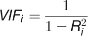where the VIF for variable is obtained using the coefficient of determination () of the regression of that variable against all other explanatory variables. Specifically, a VIF value is first calculated for each variable using the full set of explanatory variables, and the variable with the highest value is removed. Next, all VIF values with the new set of variables are recalculated, and the variable with the next highest value is removed, and so on. The above procedure is repeated until all values are below the desired threshold. As a general rule, we considered VIF > 5 as a cutoff value for the high multicollinearity problem. We used the VIF function in the “fmsb” R package to calculate VIF.

Hierarchical Cluster Analysis and PCA

Hierarchical cluster analysis (HCA) and PCA were performed to visualize the data globally. HCA builds a hierarchy from individuals by progressively merging clusters, while PCA is a technique used to reduce dimensionality of the data by finding linear combinations (dimensions; in this case, the number of traits) of the original data.

To identify plants from the same genotype or agronomic groups with similar phenotypic composition, we performed HCA with the normalized databased on the list of highly reproducible traits. All analyses were conducted with the complete linkage hierarchical clustering method and Euclidean distances and were visualized as a heat map with a dendrogram using the “heatmap.2” function of the corresponding R package.

PCA was performed to characterize each plant based on phenotypic composition and to indicate the affiliations within the phenotypic diversity of four agronomic groups. PCA was performed using Bayesian principal component analysis (the “bpca” function) as implemented in the R package pcaMethods (Stacklies et al., 2007). The first six principal components (PCs 1 to 6) and the corresponding component loading vectors (PCs 1 to 6) were visualized and summarized in scatterplots, in which principal components are coded in color and in shape according to genotypes of origin (control plants in blank points and stressed plants in filled points) and component loadings (indicated in lines) are colored according to phenotypic classification. PCA was performed for control, stress, and the total list of plants, respectively (Figure 5; Supplemental Figures 6 and 7).

Phenotypic Similarity Tree and Mantel Test

As phenotypic traits are derived from heritable characters, the influence of environmental factors and their interactions, it is possible to measure the phenotypic relationship of different genotypes based on the available traits. A “phenotypic similarity tree” was constructed to show the phenotypic relationship from a global perspective. Phenotypic similarity trees can be used to quantitatively describe the relationship of genotypes and phenotypes and to compare the differences of phenotypes under different conditions (Zhao et al., 2011). Genotypes from the DH groups were excluded from the phenotypic similarity tree analysis.

First, a phenotypic profile for each genotype was calculated as the average value from replicated plants. Next, a phenotypic distance (based on the Euclidean measure) matrix of pairwise comparisons between genotypes was estimated based on the normalized phenotypic profile. The above analysis was performed for control and stressed plants, respectively. For stressed plants, only data after DAS 34 were taken into consideration because from that time point stressed plants showed differences in their phenotypes from control plants (see the below SVM method). Finally, the phenotypic similarity trees were generated based on the distance matrices using the function “plot.phylo” implemented in the R package ape (Paradis et al., 2004).

We performed a Mantel test (Mantel, 1967) to examine the extent of correlation of the phenotypic distances between the control and stress plant sets. A positive correlation would be expected in the case that plants maintain their phenotypic similarity in different environments. We used the phenotypic distance matrixes from above to conduct the analysis. The Mantel test was computed using the function “mantel” in the corresponding R package with 10,000 permutations (Monte-Carlo simulation) and selecting Pearson’s correlation method.

Plant Classification Using SVM

Based on their phenotypic traits (features), plants from the same genotype were classified into control and stress groups (Supplemental Figure 5A), using the pairwise classification strategy of the SVM algorithm as provided by the libsvm library (Chang and Lin, 2011) via the R package e1071. The SVM classifier was used to find “optimal” hyperplanes separating two groups of plants in the multidimensional feature space. Using a linear kernel, the SVM parameters were optimized through 2-fold cross-validation to maximize the accuracy rate for classification and to minimize the mean squared error for regression. Specifically, we trained a classifier on a randomly chosen subset of half of the images (approximately nine images) from one specific genotype or treatment from one specific day (the training set) and then used the classifier to validate the other half of the images (the validation set).

ANOVA and Trait Heritability Estimation

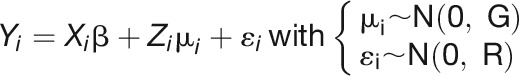
The observed variance in a particular phenotypic variable (trait) can be partitioned into components attributable to different sources of variation, for example, the variation of genotype (G), environment (E), and their interaction (G×E). The ANOVA was performed using linear mixed model (LMM) for each phenotype trait measured in each day, as defined:

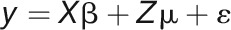where y denotes a vector of individual plant observations of a given trait; X and Z are incidence matrices associating observations with fixed effects (in vector ) and random effects (in vector ), respectively; is the vector of random residuals assuming ( is the identity matrix). Variance components for each trait, such as genotypic effect , environment effect , and their interaction effect , were estimated in the LMM using residual maximum likelihood, as implemented in ASReml-R v.3.0 (Gilmour et al., 2009). The statistical significance of variance components was estimated by the log-LR test. The statistic for the log-LR test (denoted by D) is twice the difference in the log-likelihoods of two models:

where is log-likelihood of the alternative model (with more parameters) and is log-likelihood of the null model, and both log-likelihoods can be calculated from the ASReml mixed model. Under the null hypothesis of zero correlation, the test statistic was assumed to be distributed with degrees of freedom equal the difference in number of covariance parameters estimated in the alternative versus null models. Resulting P values from LMM were corrected for multiple comparisons with the Benjamini-Hochberg false discovery rate method (Benjamini and Hochberg, 1995). We further calculated the LOD (log of odds) scores as the -log probability (corrected P value) (Joosen et al., 2013). Hierarchical clustering was applied to the matrix of LOD scores consisting traits as rows and imaging days as columns.

As a relative indicator of dispersion, we calculated the coefficient of genetic variance (CV_g) as the ratio of the sd (square root of the among-genotype variance) to the mean of the corresponding trait value across all genotypes. This analysis was performed for control plants, stress plants, and the whole set of plants, respectively (based on the mean value of control and stress plants). Similarly, the total experimental CV (CV_e) was calculated as the sum of the square root of the experimental variance, including controlled (i.e., treatment effect) and uncontrolled variation, to the mean of trait value for one specific genotype. Since CV is only reasonable to be calculated for data measured on a ratio scale (rather an interval scale), only geometric traits were considered in this calculation.

Heritability and Repeatability

The broad-sense heritability (H²) of a trait is the proportion of the total (phenotypic) variance () that is explained by the total genotypic variance () (Nyquist, 1991), which was calculated as follows:

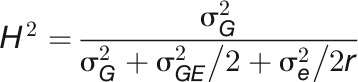where r is the average number of replications.

Repeatability (w²) is the proportion of phenotypic variance attributable to differences in repeated measures of the same genotype (in terms of replicated plants). Repeatability was calculated as 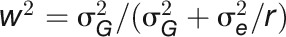, where r is the number of replicated plants. Genotypic variance was estimated by residual maximum likelihood assuming that .

Estimation of Genetic and Phenotypic Correlations

A bivariate LMM was used to estimate genetic correlations between each pair to traits (the proportion of variance that two traits share due to genetic causes) in each day. Assuming as the response vector for the subject i with the vector of measurement of the trait k (), the bivariate model is defined as follows:

where the genetic covariate matrix and the covariance matrix of measurement errors . With the assumption that and are mutually independent, it is apparent that . The genetic correlation between pairs of traits was estimated as The significance of the genetic correlation was estimated using the log-LR test by comparing the likelihood of the model allowing genetic covariance between the two traits to vary and the likelihood of the model with the genetic covariance fixed to zero. The above analyses were performed in ASReml-R v.3.0 (Gilmour et al., 2009).

Phenotypic correlations among different traits were calculated by Pearson correlation. The significance of the correlations was tested using the “cor.test” function in R.

To test the relationship between matrices of genetic and phenotypic correlations, a Mantel test (Mantel, 1967) was performed for the correlations in each day. The genetic and phenotypic correlations were visualized in networks. For visualization purpose, only significant correlations were shown (P < 0.01).

Plant Growth Modeling

Of the investigated traits, digital volume showed the best correlation with manually measured FW and DW (Supplemental Figure 8) and thus was considered to represent the digital biomass of plants. We modeled the plant growth using digital biomass for control and stressed plants, respectively.

Growth in control conditions was modeled with five different mechanistic models: linear, exponential, monomolecular, logistic, and Gompertz models (Supplemental Table 2 and Supplemental Data Set 2). To fit these models using the linear regression function “lm” in R, the nonlinear relationship of the models were first transformed into linearized forms. We fitted these linearized models using the digital volume of each control plant with the data from DAS 12 to DAS 58. The fitting quality of models was assessed and compared based on their R² and P values. Of the five models, the logistic model fitted best, with the largest R² (Supplemental Figure 9). Several useful parameters (derived traits; Supplemental Table 3) can be derived from the logistic model: (1) the intrinsic growth rate (R), which measures the speed of growth; (2) the inflection point (IP), which represents the time point when plant reaches the maximal speed of growth; and (3) the maximum final vegetative biomass (K_max), which was estimated for each plant on the basis that the model could fit the data with the largest R². To this end, K_max was initially assigned to the digital biomass at DAS 58 and the corresponding R² is calculated. The process was iterated with 1% increment of K_max at each step, and the iteration was stopped when there was no increment of R².

Modeling of growth in stress conditions is divided into two parts: (1) growth before and during the stress phase (DAS 22 to 44) and (2) regrowth during recovery phase (DAS 45 to 58). In the first phase, three different bell-shaped curves and a quadratic curve were fitted to the data, while in the recovery phase a simple linear model was used to characterize regrowth (Supplemental Table 2 and Supplemental Data Set 3). The bell-shaped models were first linearized and then fitted using the linear regression function. The bell-shaped model fitted best and was used for parameter extraction. Parameters estimated from this bell-shaped model included: time point of maximum biomass () and biomass at (Supplemental Table 3). After stress, the linear model revealed the speed of regrowth (R_rec).

Data and Software Availability

The image processing pipeline, the IAP software, is available at http://iap.ipk-gatersleben.de/. Postprocessing of image data was conducted using custom software written in R programing language (http://www.r-project.org/; release 2.15.2). The image data set, analyzed results, and corresponding R code are available at http://iap.ipk-gatersleben.de/modeling.

Supplemental Data

The following materials are available in the online version of this article.

• Supplemental Figure 1. Reproducibility of Phenotypic Traits.

• Supplemental Figure 2. Assessment of Trait Reproducibility Analysis.

• Supplemental Figure 3. Trait Similarity.

• Supplemental Figure 4. Phenotypic Traits Revealing the Stress Symptom; Related to Figure 2D.

• Supplemental Figure 5. Classification of Plants Based on the SVM Methodology.

• Supplemental Figure 6. PCA Performed over Time; Related to Figure 4B.

• Supplemental Figure 7. PCA Performed on Control and Stressed Plants, Respectively; Related to Figure 4.

• Supplemental Figure 8. Correlation Analysis of Manual Measurements with Phenotypic Traits.

• Supplemental Figure 9. Evaluation of the Performance of Growth Curves.

• Supplemental Figure 10. Comparison of stress elasticity and several drought tolerance indexes.

• Supplemental Table 1. The 54 Investigated Phenotypic Traits in This Study.

• Supplemental Table 2. Mechanistic Models Used for Modeling Biomass Accumulation in This Study.

• Supplemental Table 3. Growth Modeling of Control Plants.

• Supplemental Table 4. Growth Modeling of Stressed Plants.

• The following materials have been deposited in the DRYAD repository under accession number http://dx.doi.org/10.5061/dryad.n3215.

• Supplemental Data Set 1. Image-Derived Data Set Used in This Study.

• Supplemental Data Set 2. Growth Modeling of Control Plants.

• Supplemental Data Set 3. Growth Modeling of Stressed Plants.

Glossary

QTL

quantitative trait loci

IAP

Integrated Analysis Platform

DH

double haploid

FLUO

fluorescence

NIR

near-infrared

SVM

support vector machine

PCA

principal component analysis

PC

principal component

CV

coefficient of variation

DAS

days after sowing

FW

fresh weight

DW

dry weight

TN

tiller number

VIF

variance inflation factor

HCA

hierarchical cluster analysis

LMM

linear mixed model

log-LR

log-likelihood ratio

References

- Araus J.L., Slafer G.A., Reynolds M.P., Royo C. (2002). Plant breeding and drought in C3 cereals: what should we breed for? Ann. Bot. (Lond.) 89: 925–940. [DOI] [PMC free article] [PubMed] [Google Scholar]
- Arvidsson S., Pérez-Rodríguez P., Mueller-Roeber B. (2011). A growth phenotyping pipeline for Arabidopsis thaliana integrating image analysis and rosette area modeling for robust quantification of genotype effects. New Phytol. 191: 895–907. [DOI] [PubMed] [Google Scholar]
- Aulchenko Y.S., Ripke S., Isaacs A., van Duijn C.M. (2007). GenABEL: an R library for genome-wide association analysis. Bioinformatics 23: 1294–1296. [DOI] [PubMed] [Google Scholar]
- Baker N.R. (2008). Chlorophyll fluorescence: a probe of photosynthesis in vivo. Annu. Rev. Plant Biol. 59: 89–113. [DOI] [PubMed] [Google Scholar]
- Benjamini Y., Hochberg Y. (1995). Controlling the false discovery rate: a practical and powerful approach to multiple testing. J. R. Stat. Soc. B 57: 289–300. [Google Scholar]
- Berger B., Parent B., Tester M. (2010). High-throughput shoot imaging to study drought responses. J. Exp. Bot. 61: 3519–3528. [DOI] [PubMed] [Google Scholar]
- Biskup B., Scharr H., Fischbach A., Wiese-Klinkenberg A., Schurr U., Walter A. (2009). Diel growth cycle of isolated leaf discs analyzed with a novel, high-throughput three-dimensional imaging method is identical to that of intact leaves. Plant Physiol. 149: 1452–1461. [DOI] [PMC free article] [PubMed] [Google Scholar]
- Blackman V. (1919). The compound interest law and plant growth. Ann. Bot. (Lond.) 3: 353–360. [Google Scholar]
- Bouslama M., Schapaugh W.T. (1984). Stress tolerance in soybeans. 1. Evaluation of 3 screening techniques for heat and drought tolerance. Crop Sci. 24: 933–937. [Google Scholar]
- Busemeyer L., Ruckelshausen A., Möller K., Melchinger A.E., Alheit K.V., Maurer H.P., Hahn V., Weissmann E.A., Reif J.C., Würschum T. (2013). Precision phenotyping of biomass accumulation in triticale reveals temporal genetic patterns of regulation. Sci. Rep. 3: 2442. [DOI] [PMC free article] [PubMed] [Google Scholar]
- Bylesjö M., Segura V., Soolanayakanahally R.Y., Rae A.M., Trygg J., Gustafsson P., Jansson S., Street N.R. (2008). LAMINA: a tool for rapid quantification of leaf size and shape parameters. BMC Plant Biol. 8: 82. [DOI] [PMC free article] [PubMed] [Google Scholar]
- Calderini, D., Savin, R., Abeledo, L., Reynolds, M., and Slafer, G. (2001). The importance of the period immediately preceding anthesis for grain weight determination in wheat. In Wheat in a Global Environment, Z. Bedö and L. Láng, eds (Dordrecht, The Netherlands: Springer), pp. 503–509. [Google Scholar]
- Camargo A., Papadopoulou D., Spyropoulou Z., Vlachonasios K., Doonan J.H., Gay A.P. (2014). Objective definition of rosette shape variation using a combined computer vision and data mining approach. PLoS ONE 9: e96889. [DOI] [PMC free article] [PubMed] [Google Scholar]
- Chang C.C., Lin C.J. (2011). LIBSVM: A Library for Support Vector Machines. ACM Trans. Intell. Syst. Technol. 2: 1–27. [Google Scholar]
- Chen Y., Lübberstedt T. (2010). Molecular basis of trait correlations. Trends Plant Sci. 15: 454–461. [DOI] [PubMed] [Google Scholar]
- Damgaard C., Weiner J. (2008). Modeling the growth of individuals in crowded plant populations. J. Plant Ecol. 1: 111–116. [DOI] [PubMed] [Google Scholar]
- Davey J.W., Hohenlohe P.A., Etter P.D., Boone J.Q., Catchen J.M., Blaxter M.L. (2011). Genome-wide genetic marker discovery and genotyping using next-generation sequencing. Nat. Rev. Genet. 12: 499–510. [DOI] [PubMed] [Google Scholar]
- De Vylder J., Vandenbussche F., Hu Y., Philips W., Van Der Straeten D. (2012). Rosette tracker: an open source image analysis tool for automatic quantification of genotype effects. Plant Physiol. 160: 1149–1159. [DOI] [PMC free article] [PubMed] [Google Scholar]
- Dhondt S., Wuyts N., Inzé D. (2013). Cell to whole-plant phenotyping: the best is yet to come. Trends Plant Sci. 18: 428–439. [DOI] [PubMed] [Google Scholar]
- Eberius M.,. andLima-Guerra J. (2009). High-throughput plant phenotyping: Data acquisition, transformation, and analysis. In Bioinformatics: Tools and Applications, Edwards D., Stajich J., and Hansen D., eds (New York: Springer; ), pp. 259–278. [Google Scholar]
- Edwards D., Batley J., Snowdon R.J. (2013). Accessing complex crop genomes with next-generation sequencing. Theor. Appl. Genet. 126: 1–11. [DOI] [PubMed] [Google Scholar]
- El-Lithy M.E., Clerkx E.J., Ruys G.J., Koornneef M., Vreugdenhil D. (2004). Quantitative trait locus analysis of growth-related traits in a new Arabidopsis recombinant inbred population. Plant Physiol. 135: 444–458. [DOI] [PMC free article] [PubMed] [Google Scholar]
- Erickson R.O. (1976). Modeling of plant growth. Annu. Rev. Plant Physiol. 27: 407–434. [Google Scholar]
- Fiorani F., Schurr U. (2013). Future scenarios for plant phenotyping. Annu. Rev. Plant Biol. 64: 267–291. [DOI] [PubMed] [Google Scholar]
- Fischer R.A., Maurer R. (1978). Drought resistance in spring wheat cultivars. 1. Grain-yield responses. Aust. J. Agric. Res. 29: 897–912. [Google Scholar]
- Furbank R.T., Tester M. (2011). Phenomics—technologies to relieve the phenotyping bottleneck. Trends Plant Sci. 16: 635–644. [DOI] [PubMed] [Google Scholar]
- Gilmour A.R., Gogel B., Cullis B., Thompson R. (2009). ASReml User Guide Release 3.0. (Hemel Hempstead, UK: VSN International; ). [Google Scholar]
- Golzarian M.R., Frick R.A., Rajendran K., Berger B., Roy S., Tester M., Lun D.S. (2011). Accurate inference of shoot biomass from high-throughput images of cereal plants. Plant Methods 7: 2. [DOI] [PMC free article] [PubMed] [Google Scholar]
- Gompertz B. (1825). On the nature of the function expressive of the law of human mortality, and on a new mode of determining the value of life contingencies. Philos. Trans. R. Soc. Lond. 115: 513–583. [DOI] [PMC free article] [PubMed] [Google Scholar]
- Granier C., et al. (2006). PHENOPSIS, an automated platform for reproducible phenotyping of plant responses to soil water deficit in Arabidopsis thaliana permitted the identification of an accession with low sensitivity to soil water deficit. New Phytol. 169: 623–635. [DOI] [PubMed] [Google Scholar]
- Green J.M., Appel H., Rehrig E.M., Harnsomburana J., Chang J.F., Balint-Kurti P., Shyu C.R. (2012). PhenoPhyte: a flexible affordable method to quantify 2D phenotypes from imagery. Plant Methods 8: 45. [DOI] [PMC free article] [PubMed] [Google Scholar]
- Grubbs F.E. (1950). Sample criteria for testing outlying observations. J. Am. Stat. Assoc. 21: 27–58. [Google Scholar]
- Hartmann A., Czauderna T., Hoffmann R., Stein N., Schreiber F. (2011). HTPheno: an image analysis pipeline for high-throughput plant phenotyping. BMC Bioinformatics 12: 148. [DOI] [PMC free article] [PubMed] [Google Scholar]
- Holland J.B., Nyquist W.E., Cervantes-Martínez C.T. (2003). Estimating and interpreting heritability for plant breeding: An update. Plant Breed. Rev. 22: 9–112. [Google Scholar]
- Houle D., Govindaraju D.R., Omholt S. (2010). Phenomics: the next challenge. Nat. Rev. Genet. 11: 855–866. [DOI] [PubMed] [Google Scholar]
- Hunt R. (1982). Plant growth curves: the functional approach to plant growth analysis. (London: Edward Arnold; ). [Google Scholar]
- Iyer-Pascuzzi A.S., Symonova O., Mileyko Y., Hao Y., Belcher H., Harer J., Weitz J.S., Benfey P.N. (2010). Imaging and analysis platform for automatic phenotyping and trait ranking of plant root systems. Plant Physiol. 152: 1148–1157. [DOI] [PMC free article] [PubMed] [Google Scholar]
- Jansen M., et al. (2009). Simultaneous phenotyping of leaf growth and chlorophyll fluorescence via GROWSCREEN FLUORO allows detection of stress tolerance in Arabidopsis thaliana and other rosette plants. Funct. Plant Biol. 36: 902–914. [DOI] [PubMed] [Google Scholar]
- Joosen R.V., Arends D., Li Y., Willems L.A., Keurentjes J.J., Ligterink W., Jansen R.C., Hilhorst H.W. (2013). Identifying genotype-by-environment interactions in the metabolism of germinating arabidopsis seeds using generalized genetical genomics. Plant Physiol. 162: 553–566. [DOI] [PMC free article] [PubMed] [Google Scholar]
- Kang H.M., Zaitlen N.A., Wade C.M., Kirby A., Heckerman D., Daly M.J., Eskin E. (2008). Efficient control of population structure in model organism association mapping. Genetics 178: 1709–1723. [DOI] [PMC free article] [PubMed] [Google Scholar]
- Karadavut U., Kayis S.A., Palta Ç, Okur O. (2008). A growth curve application to compare plant heights and dry weights of some wheat varieties, American-Eurasian. J. Agric. Environ. Sci. 3: 888–892. [Google Scholar]
- Karadavut U., Palta Ç., Kokten K., Bakoglu A. (2010). Comparative study on some non-linear growth models for describing leaf growth of maize. Int. J. Agric. Biol. 12: 227–230. [Google Scholar]
- Karaletsos T., Stegle O., Dreyer C., Winn J., Borgwardt K.M. (2012). ShapePheno: unsupervised extraction of shape phenotypes from biological image collections. Bioinformatics 28: 1001–1008. [DOI] [PubMed] [Google Scholar]
- Karkach A. (2006). Trajectories and models of individual growth. Demogr. Res. 15: 347–400. [Google Scholar]
- Klukas C., Chen D., Pape J.M. (2014). Integrated Analysis Platform: An open-source information system for high-throughput plant phenotyping. Plant Physiol. 165: 506–518. [DOI] [PMC free article] [PubMed] [Google Scholar]
- Knipling E.B. (1970). Physical and physiological basis for the reflectance of visible and near-infrared radiation from vegetation. Remote Sens. Environ. 1: 155–159. [Google Scholar]
- Kohonen T. (1990). The self-organizing map. Proc. IEEE 78: 1464–1480. [Google Scholar]
- Lilley J., Ludlow M., McCouch S., O'Toole J. (1996). Locating QTL for osmotic adjustment and dehydration tolerance in rice. J. Exp. Bot. 47: 1427–1436. [Google Scholar]
- Lipka A.E., Tian F., Wang Q., Peiffer J., Li M., Bradbury P.J., Gore M.A., Buckler E.S., Zhang Z. (2012). GAPIT: genome association and prediction integrated tool. Bioinformatics 28: 2397–2399. [DOI] [PubMed] [Google Scholar]
- Loo L.H., Wu L.F., Altschuler S.J. (2007). Image-based multivariate profiling of drug responses from single cells. Nat. Methods 4: 445–453. [DOI] [PubMed] [Google Scholar]
- Mantel N. (1967). The detection of disease clustering and a generalized regression approach. Cancer Res. 27: 209–220. [PubMed] [Google Scholar]
- Meade K.A., Cooper M., Beavis W.D. (2013). Modeling biomass accumulation in maize kernels. Field Crops Res. 151: 92–100. [Google Scholar]
- Meijón M., Satbhai S.B., Tsuchimatsu T., Busch W. (2014). Genome-wide association study using cellular traits identifies a new regulator of root development in Arabidopsis. Nat. Genet. 46: 77–81. [DOI] [PubMed] [Google Scholar]
- Moore C.R., Johnson L.S., Kwak I.Y., Livny M., Broman K.W., Spalding E.P. (2013). High-throughput computer vision introduces the time axis to a quantitative trait map of a plant growth response. Genetics 195: 1077–1086. [DOI] [PMC free article] [PubMed] [Google Scholar]
- Munns R., James R.A., Sirault X.R., Furbank R.T., Jones H.G. (2010). New phenotyping methods for screening wheat and barley for beneficial responses to water deficit. J. Exp. Bot. 61: 3499–3507. [DOI] [PubMed] [Google Scholar]
- Nagel K.A., et al. (2012). GROWSCREEN-Rhizo is a novel phenotyping robot enabling simultaneous measurements of root and shoot growth for plants grown in soil-filled rhizotrons. Funct. Plant Biol. 39: 891–904. [DOI] [PubMed] [Google Scholar]
- Nezhad K.Z., Weber W., Röder M., Sharma S., Lohwasser U., Meyer R., Saal B., Börner A. (2012). QTL analysis for thousand-grain weight under terminal drought stress in bread wheat (Triticum aestivum L.). Euphytica 186: 127–138. [Google Scholar]
- Nyquist W.E. (1991). Estimation of heritability and prediction of selection response in plant populations. Crit. Rev. Plant Sci. 10: 235–322. [Google Scholar]
- O'Brien R.M. (2007). A caution regarding rules of thumb for variance inflation factors. Qual. Quant. 41: 673–690. [Google Scholar]
- Painawadee M., Jogloy S., Kesmala T., Akkasaeng C., Patanothai A. (2009). Heritability and correlation of drought resistance traits and agronomic traits in peanut (Arachis hypogaea L.). Asian J. Plant Sci. 8: 325–334. [Google Scholar]
- Paine C.E.T., Marthews T.R., Vogt D.R., Purves D., Rees M., Hector A., Turnbull L.A. (2012). How to fit nonlinear plant growth models and calculate growth rates: an update for ecologists. Methods Ecol. Evol. 3: 245–256. [Google Scholar]
- Paproki A., Sirault X., Berry S., Furbank R., Fripp J. (2012). A novel mesh processing based technique for 3D plant analysis. BMC Plant Biol. 12: 63. [DOI] [PMC free article] [PubMed] [Google Scholar]
- Paradis E., Claude J., Strimmer K. (2004). APE: Analyses of Phylogenetics and Evolution in R language. Bioinformatics 20: 289–290. [DOI] [PubMed] [Google Scholar]
- Paul-Victor C., Züst T., Rees M., Kliebenstein D.J., Turnbull L.A. (2010). A new method for measuring relative growth rate can uncover the costs of defensive compounds in Arabidopsis thaliana. New Phytol. 187: 1102–1111. [DOI] [PubMed] [Google Scholar]
- Porth I., Klápště J., Skyba O., Lai B.S., Geraldes A., Muchero W., Tuskan G.A., Douglas C.J., El-Kassaby Y.A., Mansfield S.D. (2013). Populus trichocarpa cell wall chemistry and ultrastructure trait variation, genetic control and genetic correlations. New Phytol. 197: 777–790. [DOI] [PubMed] [Google Scholar]
- Rajendran K., Tester M., Roy S.J. (2009). Quantifying the three main components of salinity tolerance in cereals. Plant Cell Environ. 32: 237–249. [DOI] [PubMed] [Google Scholar]
- Reymond M., Muller B., Leonardi A., Charcosset A., Tardieu F. (2003). Combining quantitative trait Loci analysis and an ecophysiological model to analyze the genetic variability of the responses of maize leaf growth to temperature and water deficit. Plant Physiol. 131: 664–675. [DOI] [PMC free article] [PubMed] [Google Scholar]
- Ribaut J.-M., Jiang C., Gonzalez-de-Leon D., Edmeades G., Hoisington D. (1997). Identification of quantitative trait loci under drought conditions in tropical maize. 2. Yield components and marker-assisted selection strategies. Theor. Appl. Genet. 94: 887–896. [Google Scholar]
- Schadt E.E., Linderman M.D., Sorenson J., Lee L., Nolan G.P. (2010). Computational solutions to large-scale data management and analysis. Nat. Rev. Genet. 11: 647–657. [DOI] [PMC free article] [PubMed] [Google Scholar]
- Seelig H.D., Hoehn A., Stodieck L.S., Klaus D.M., Adams W.W., Emery W.J. (2008). The assessment of leaf water content using leaf reflectance ratios in the visible, near-, and short-wave-infrared. Int. J. Remote Sens. 29: 3701–3713. [Google Scholar]
- Seelig H.D., Hoehn A., Stodieck L.S., Klaus D.M., Adams W.W., Emery W.J. (2009). Plant water parameters and the remote sensing R (1300)/R (1450) leaf water index: controlled condition dynamics during the development of water deficit stress. Irrig. Sci. 27: 357–365. [Google Scholar]
- Sellammal R., Robin S., Raveendran M. (2014). Association and heritability studies for drought resistance under varied moisture stress regimes in backcross inbred population of rice. Rice Sci. 21: 150–161. [Google Scholar]
- Slovak R., Göschl C., Su X., Shimotani K., Shiina T., Busch W. (2014). A scalable open-source pipeline for large-scale root phenotyping of Arabidopsis. Plant Cell 26: 2390–2403. [DOI] [PMC free article] [PubMed] [Google Scholar]
- Sozzani R., Benfey P.N. (2011). High-throughput phenotyping of multicellular organisms: finding the link between genotype and phenotype. Genome Biol. 12: 219. [DOI] [PMC free article] [PubMed] [Google Scholar]
- Stacklies W., Redestig H., Scholz M., Walther D., Selbig J. (2007). pcaMethods—a bioconductor package providing PCA methods for incomplete data. Bioinformatics 23: 1164–1167. [DOI] [PubMed] [Google Scholar]
- Stackpole D.J., Vaillancourt R.E., Alves A., Rodrigues J., Potts B.M. (2011). Genetic variation in the chemical components of Eucalyptus globulus wood. G3 (Bethesda) 1: 151–159. [DOI] [PMC free article] [PubMed] [Google Scholar]
- Sultan S.E. (2000). Phenotypic plasticity for plant development, function and life history. Trends Plant Sci. 5: 537–542. [DOI] [PubMed] [Google Scholar]
- Szira F., Bálint A., Börner A., Galiba G. (2008). Evaluation of drought‐Related traits and screening methods at different developmental stages in spring barley. J. Agron. Crop Sci. 194: 334–342. [Google Scholar]
- Tardieu F., Tuberosa R. (2010). Dissection and modelling of abiotic stress tolerance in plants. Curr. Opin. Plant Biol. 13: 206–212. [DOI] [PubMed] [Google Scholar]
- Tessmer O.L., Jiao Y., Cruz J.A., Kramer D.M., Chen J. (2013). Functional approach to high-throughput plant growth analysis. BMC Syst. Biol. 7 (suppl. 6): S17. [DOI] [PMC free article] [PubMed] [Google Scholar]
- Thornley J.H.,. andFrance J. (2007). Mathematical Models in Agriculture: Quantitative Methods for the Plant, Animal and Ecological Sciences, 2nd ed. (Wallingford, UK: CABI; ). [Google Scholar]
- Tuberosa R. (2012). Phenotyping for drought tolerance of crops in the genomics era. Front. Physiol 3: 347. [DOI] [PMC free article] [PubMed] [Google Scholar]
- Tucker C.J. (1980). Remote sensing of leaf water content in the near infrared. Remote Sens. Environ. 10: 23–32. [Google Scholar]
- Vanclay J.K. (1994). Modelling Forest Growth and Yield: Applications to Mixed Tropical Forests. (Wallingford, UK: CABI; ). [Google Scholar]
- Van Poecke R.M., Sato M., Lenarz-Wyatt L., Weisberg S., Katagiri F. (2007). Natural variation in RPS2-mediated resistance among Arabidopsis accessions: correlation between gene expression profiles and phenotypic responses. Plant Cell 19: 4046–4060. [DOI] [PMC free article] [PubMed] [Google Scholar]
- Visscher P.M., Hill W.G., Wray N.R. (2008). Heritability in the genomics era—concepts and misconceptions. Nat. Rev. Genet. 9: 255–266. [DOI] [PubMed] [Google Scholar]
- Walter A., Scharr H., Gilmer F., Zierer R., Nagel K.A., Ernst M., Wiese A., Virnich O., Christ M.M., Uhlig B., Jünger S., Schurr U. (2007). Dynamics of seedling growth acclimation towards altered light conditions can be quantified via GROWSCREEN: a setup and procedure designed for rapid optical phenotyping of different plant species. New Phytol. 174: 447–455. [DOI] [PubMed] [Google Scholar]
- Wang L., Uilecan I.V., Assadi A.H., Kozmik C.A., Spalding E.P. (2009). HYPOTrace: image analysis software for measuring hypocotyl growth and shape demonstrated on Arabidopsis seedlings undergoing photomorphogenesis. Plant Physiol. 149: 1632–1637. [DOI] [PMC free article] [PubMed] [Google Scholar]
- Weight C., Parnham D., Waites R. (2008). LeafAnalyser: a computational method for rapid and large-scale analyses of leaf shape variation. Plant J. 53: 578–586. [DOI] [PubMed] [Google Scholar]
- Woo N.S., Badger M.R., Pogson B.J. (2008). A rapid, non-invasive procedure for quantitative assessment of drought survival using chlorophyll fluorescence. Plant Methods 4: 27. [DOI] [PMC free article] [PubMed] [Google Scholar]
- Wu R., Lin M. (2006). Functional mapping - how to map and study the genetic architecture of dynamic complex traits. Nat. Rev. Genet. 7: 229–237. [DOI] [PubMed] [Google Scholar]
- Xiong L., Wang R.G., Mao G., Koczan J.M. (2006). Identification of drought tolerance determinants by genetic analysis of root response to drought stress and abscisic acid. Plant Physiol. 142: 1065–1074. [DOI] [PMC free article] [PubMed] [Google Scholar]
- Yang W., et al. (2014). Combining high-throughput phenotyping and genome-wide association studies to reveal natural genetic variation in rice. Nat. Commun. 5: 5087. [DOI] [PMC free article] [PubMed] [Google Scholar]
- Yin X., Struik P.C., Tang J., Qi C., Liu T. (2005a). Model analysis of flowering phenology in recombinant inbred lines of barley. J. Exp. Bot. 56: 959–965. [DOI] [PubMed] [Google Scholar]
- Yin X., Struik P.C., van Eeuwijk F.A., Stam P., Tang J. (2005b). QTL analysis and QTL-based prediction of flowering phenology in recombinant inbred lines of barley. J. Exp. Bot. 56: 967–976. [DOI] [PubMed] [Google Scholar]
- Zeide B. (1993). Analysis of growth equations. Forest Sci. 39: 594–616. [Google Scholar]
- Zhang X., Hause R.J. Jr., Borevitz J.O. (2012). Natural genetic variation for growth and development revealed by high-throughput phenotyping in Arabidopsis thaliana. G3 (Bethesda) 2: 29–34. [DOI] [PMC free article] [PubMed] [Google Scholar]
- Zhao K., et al. (2011). Genome-wide association mapping reveals a rich genetic architecture of complex traits in Oryza sativa. Nat. Commun. 2: 467. [DOI] [PMC free article] [PubMed] [Google Scholar]
- Züst T., Joseph B., Shimizu K.K., Kliebenstein D.J., Turnbull L.A. (2011). Using knockout mutants to reveal the growth costs of defensive traits. Proc. Biol. Sci. 278: 2598–2603. [DOI] [PMC free article] [PubMed] [Google Scholar]
Associated Data
This section collects any data citations, data availability statements, or supplementary materials included in this article.