Dosage Effects of Salt and pH Stresses on Saccharomyces cerevisiae as Monitored via Metabolites by Using Two Dimensional NMR Spectroscopy

Abstract

Saccharomyces cerevisiae, which is a common species of yeast, is by far the most extensively studied model of a eukaryote because although it is one of the simplest eukaryotes, its basic cellular processes resemble those of higher organisms. In addition, yeast is a commercially valuable organism for ethanol production. Since the yeast data can be extrapolated to the important aspects of higher organisms, many researchers have studied yeast metabolism under various conditions. In this report, we analyzed and compared metabolites of Saccharomyces cerevisiae under salt and pH stresses of various strengths by using two-dimensional NMR spectroscopy. A total of 31 metabolites were identified for most of the samples. The levels of many identified metabolites showed gradual or drastic increases or decreases depending on the severity of the stresses involved. The statistical analysis produced a holistic outline: pH stresses were clustered together, but salt stresses were spread out depending on the severity. This work could provide a link between the metabolite profiles and mRNA or protein profiles under representative and well studied stress conditions.

Introduction

Saccharomyces cerevisiae can be regarded the most extensively studied model of eukaryotes for many different kinds of studies since its basic cellular processes are similar to those of higher eukaryotic organisms, including humans.^1,2 From a commercial point of view, yeast is a valuable organism for the production of ethanol which can be used as food or fuel.^3,4 Among several important and interesting studies, those studies on yeast metabolism are focused on its response to specific stress conditions because the results can be extended to other higher eukaryotes. For example, oxidative stress is thought to be related to aging, apoptosis, cancer, or immunological responses.⁵

Yeast cells express a common set of genes to protect themselves during stressful periods. This phenomenon is called the environmental stress response (ESR), which includes activation or suppression of around 900 genes.⁶ In addition to the general physiological response, the expressions of those genes are precisely coordinated to protect the cells against the specific nature of the stress.⁶ The response and adaptation of yeast to various stress conditions including ethanol,⁷ osmotic stress,⁸ oxidative stress,⁹ extreme pHs⁹ and heat shock^8,10,11 have been well established. Recently, Berry and Gasch reported that any single stress could trigger the change of the gene expression not only to cope with the given stress but also to prepare for possible future stresses.¹²

Most of those works have been accomplished through functional genomics studies by observing the changes of gene expression patterns or mRNA levels. However, these changes may not show a linear correlation with protein or metabolite levels.¹³ In one report, there was little agreement between the gene expression and metabolite concentrations in the liver, urine, or plasma.¹⁴ In another report, metabolic data was employed in the functional genomic strategy to reveal the phenotype of silent mutations.¹⁵ Recently, efforts have been made to integrate the “Omics” technologies to describe organisms in a holistic and systematic way.^16,17

Metabolomics is the “systematic study of the unique chemical fingerprints that specific cellular processes leave behind,” or more specifically, the study of their small-molecule metabolite profiles.¹⁸ The metabolome represents a collection of all end products of the gene expression in a biological organism.¹⁹ For many organisms, including yeast, the number of metabolites is far fewer than that of genes or gene products.¹⁵ Thus, metabolic profiling can provide a simpler yet efficient snapshot of the system’s physiology. Researchers around the world have been developing various metabolome databases to offer faster identification of interesting metabolites and their corresponding properties. There are several databases that are open to the public: HMDB,²⁰ MMCD,²¹ METLIN,²² YMDB,²³ MDL (http://mdl.imv.liu.se), and PRiMe.²⁴ YMDB (Yeast Metabolome Database) is a specialized database for yeast metabolome.

One-dimensional ¹H nuclear magnetic resonance (NMR) spectroscopy has been used extensively as an analytical tool for identifying and quantifying small molecules.²⁵ When samples contain minimal peak overlap, 1D ¹H NMR can be employed because the peak intensity and its concentration maintain a linear relationship. Recently, high throughput analysis of complex biological processes at the metabolic level by NMR has been receiving a great deal of attention. These studies, however, rely on 1D ¹H NMR, and inevitably suffer from extensive peak overlap. As an alternative to the metabolomics by 1D NMR, a two-dimensional ¹H-¹³C HSQC (Heteronuclear Single Quantum Coherence) has been proposed, and this method has shown promising results towards obtaining quantitative data of metabolite concentrations.²⁵ However, the semi-quantitative analysis like this report would suffice in many cases because the research was focused on differentiating responses from different stresses.

In this work, we applied several common stresses to yeast cultures to see if we could classify those stresses in terms of the metabolite profiles (or specific markers) and if the result could be integrated with currently available functional genomic data. This work could provide a link between the metabolite profiles and mRNA or protein profiles under representative and well studied stress conditions.

Materials and Methods

Yeast Growth

W303 (MATa/MATα (leu2-3,112 trp1-1 can1-100 ura3-1 ade2-1 his3-11,15) [phi+]), a commonly used strain of Saccharomyces cerevisiae, was grown in YPD medium (1% yeast extract, 2% bactopeptone, and 2% glucose). For seed cultivation, yeast cells were grown overnight in 5 mL YPD at 30 °C. For the main cultivation, the pre-cultivated cells were inoculated into 500 mL of fresh medium in a 2.8 L baffled Fernbach flask at an initial OD₆₀₀ of approximately 0.07 and cultivated for 24 h under salt or pH stress conditions. The salt stress conditions were imposed by adding NaCl to the concentrations of 0.2, 0.4, 0.8, 1.0 M. The pH stress conditions were imposed by adjusting the culture pH to 2.4, 3.4, 4.1, 5.0, 6.0, and 7.1. The cultures were harvested by centrifugation at 3380 g at 4 °C for 20 minutes. Cells were resuspended in a 100 mL PBS buffer (10 mM sodium phosphate, 150 mM NaCl, pH 7.4) and centrifuged at 4000 g at 4 °C for 20 minutes. The cell washing step was repeated twice. Cell pellets were stored at −70 °C. Frozen pellets were lyophilized later.

Metabolite Extraction and NMR Sample Preparation

15 mL of boiling deionized water was added to a dried cell pellet in a 50 mL conical tube. The mixture was incubated at 121 °C for 20 minutes in an autoclave, then cooled on ice, and then centrifuged at 4000 g at 4 °C for 10 minutes. Fine debris was removed with 0.45 μm pore syringe filters. The resulting filtrate was then transferred to VIVASPIN 20 centrifugal filters (MWCO 5000 Da, Sartorius Stedim, Bohemia, NY, USA) and centrifuged at 4000 g at 4 °C until less than 0.5 mL of solution remained in the upper compartment. The syringe filters and centrifugal filters were washed with 10 mL water 3 times before use. The final filtrate was frozen and lyophilized. The dried extract powder was weighed and dissolved in 0.5 mL HEPES buffer (5 mM HEPES, 0.2 mM DSS, 0.5 mM NaN₃ in D₂O). The pH was adjusted to 7.40 ± 0.05.

NMR Data Collection and Data Processing

NMR data were collected at the National Magnetic Resonance Facility at Madison on a Bruker Avance III instrument operating at 600.133 MHz equipped with a triple-resonance (¹H, ¹³C, ¹⁵N, ²H lock) 1.7 mm cryogenic probe and a SampleJet. All samples were centrifuged at maximum speed for 5 min prior to placing them into NMR tubes. After inserting each sample into the spectrometer, we waited 120 s to allow the sample to reach thermal equilibrium. The probe was tuned, matched and locked to deuterium for the first sample; the lock signal was adjusted automatically as needed. All samples were collected using automated shimming and manual shimming as needed to obtain a 50% linewidth on DSS less than 1 Hz. The optimal 90° pulsewidth was determined manually for each sample and the receiver gain was automatically calculated. One-dimensional ¹H were collected with excitation sculpting using the water-selective 180° zgesgp pulse sequence from the Bruker pulse sequence library; spectra were collected at 298 K with 2 steady state scans, 16 transients, 2560 complex points, a spectral width of 10.5 ppm and an interscan delay of 1.75 s. Two-dimensional ¹H-¹³C HSQC (Heteronuclear Single Quantum Coherence) spectra were collected using the hsqcetgpsisp2.2 pulse sequence from the Bruker pulse sequence library. All spectra were collected at 298 K with 4 transients, 32 steady state scans, GARP (Globally-optimized Alternating-phase Rectangular Pulses) broadband decoupling and a 1.75 s interscan delay time; 1262 complex data points were collected in the direct dimension (¹H) with a spectral width of 10.5 ppm (6313 Hz); 256 complex data points were collected in the indirect dimension (¹³C) with a spectral width of 99.5 ppm (15015 Hz). The resulting spectra were processed by NMRPipe,²⁶ and visualized and analyzed by rNMR.²⁷ The peaklist was sent to MMCD (Madison Metabolomics Consortium Database, http://mmcd.nmrfam.wisc.edu) to find candidate metabolites. With the help of the in-house software (S. H. Kim and Y. K. Chae, unpublished data), the peak intensity data were first corrected for dilution that occurred when dissolving dried extract in HEPES buffer and adjusting pH, then normalized to one of the peaks of the internal standard HEPES, then adjusted to the sample mass, and processed to yield a proper output format for the multivariate analysis. The multivariate analysis was performed with the R statistics software package (http://www.r-project.org).

Results and Discussion

Sample Preparation

The cultures were harvested when the optical density at 600 nm did not change any further. This was to ensure not only that the cells were entirely in their stationary phase, but also that they did not yet enter the death phase. When to harvest the culture was determined by considering two conditions: we intended to observe the accumulated effect and to equalize the final growth state of each stress condition. However, since each given stress had its own severity, the final optical densities and dried masses of the cultures varied to some degree (data not shown), which resulted in the different amounts of dried extract (Table 1). The rich medium (YPD) was chosen as a growth medium because we tried to focus on the specific stresses such as NaCl and pH, and did not want the cells to experience nutrient-limiting stress in the minimal medium. These two background factors (the stationary phase and the rich medium) offered a window through which we could observe the accumulated effect of only the specific stresses at the analysis stage because we had a control sample without the stress. The underlying assumption was that the background factors were common to every sample so that the common effects could be subtracted to reveal the true differences.

Table 1.

Summary of dried extract mass from 12 different conditions

Stress condition	Dried extract mass (mg)	Stress condition	Dried extract mass (mg)
Control	224.4	pH 2.4	88.9
0.2 M NaCl	381.2	pH 3.4	106.9
0.4 M NaCl	250.8	pH 4.1	109.7
0.6 M NaCl	309.9	pH 5.0	103.4
0.8 M NaCl	223.4	pH 6.1	129.7
1.0 M NaCl	81	pH 7.1	136.9

Addition of 15 mL of boiling water to the dried raw material not only ensured the denaturation of endogenous enzymes that might degrade or synthesize metabolites during the extraction procedure but also served a sanitary purpose. The resulting mixture was autoclaved for 20 min, and only the small, soluble and heat-resistant metabolites that exuded out of the cells were collected for NMR analysis. Although it is possible that the heat-labile metabolites could have been disintegrated into simpler compounds during the hot water extraction procedure, there is a controversy over the best extraction method for metabolite profiling, especially among hot water, chloroform-methanol, and boiling ethanol.^28–31 Despite the concern of hydrolysis of the macromolecules or phosphorylated compounds, the hot water extraction method was the choice regarding sensitivity over resolution, that is, we chose to achieve a higher total glucose signal instead of every glucose-containing compound. Although the hot water extraction was hard on the condition of the dried cells, only a small fraction of them were lysed. This was judged by the observation of a clear supernatant after centrifugation at 4000 g, which was not fast enough to spin down fine debris. As shown in Table 1, the harsher the growth condition was, the less extract we could obtain, which is understandable because harsher conditions prevented further cell growth. The NMR samples were prepared by adding an equal volume of HEPES buffer, and the difference in the extract amount was compensated in the analysis stage.

NMR Data Collection and Processing

Each 2D HSQC experiment took about 2 h. Due to the small sample volume (45 μL) for the 1.7 mm probe, GARP decoupling during acquisition raised the sample temperature, which made it necessary to use a longer delay time between scans (1.75 s) than the usual (1 s). However, we were able to take advantage of the small sample volume, that is, we could use a more concentrated sample. Despite the longer data collection time, 2D NMR can be considered as a potent alternative to 1D NMR for higher accuracy and robustness.^32–35 The cryoprobe and autosampler drastically reduced the data collection time down to 2 h, which otherwise would have been much longer.

NMR Data Analysis

A portion of the NMR spectrum of a control sample along with the assignments of identified metabolites is shown in Figure 1, and various methylene groups usually appear in this region. From the combined use of rNMR and public databases such as MMCD, HMDB, and PRIMe, 31 metabolites were identified by observing multiple peaks of each given metabolite. When assigning a spectrum, MMCD was the first database to be consulted, and unassigned resonances were assigned by consulting HMDB and PRIMe. This process was not only helpful but also necessary because different databases complemented one another. In Figure 2, the representative signals of the identified metabolites are shown, and this is the view that overlooks all the 2D spectra: only the ones that will further be used for statistical analysis are shown (resonances-of-interest or ROIs). There is one caveat that we need to consider when we look at this ROI view: Those resonances show the original intensities before the necessary calibrations are applied, that is, we need to compensate intensity variations in signals resulting from NMR experiments and differences in total metabolite concentrations among samples. As for the errors in NMR experiments, the signals were normalized by the representative HEPES resonance which was present in every NMR sample at the same concentration (5 mM). Then the concentration differences were compensated by dividing signal intensities by the mass of extracted metabolites. Figure 3 is the result of this process for more accurate comparison among samples.

Figure 1.

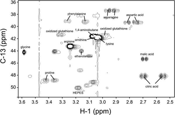
The upfield portion of the two-dimensional ¹H-¹³C HSQC spectrum of the control sample. The assigned resonances are labeled with the names of the corresponding metabolites.

Figure 2.

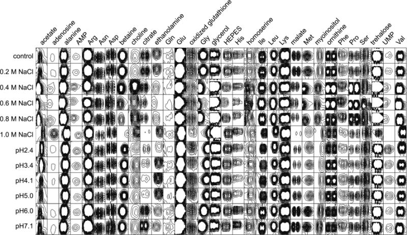
ROI view of the representative resonances of identified metabolites. This view shows the raw data before the two normalization steps against HEPES and the concentration were applied.

Figure 3.

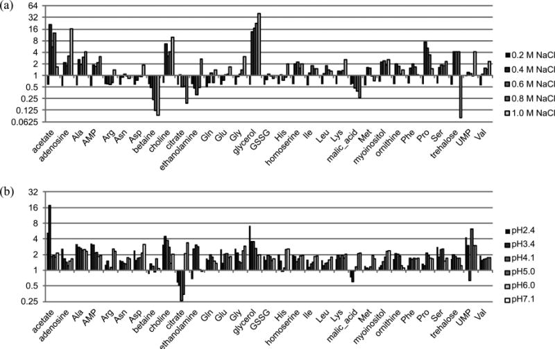
Changes of resonance intensities under salt stress (a) and pH stress (b). Individual intensities were divided by those of the control.

We could observe several peculiar features regarding the concentration changes of various metabolites which should reflect the intracellular environment in Figure 3. First of all, three well-known osmoprotectants showed completely different behaviors: Betaine gradually decreased to reach its minimum at 1.0 M NaCl, and glycerol showed a large increase even at 0.2 M NaCl and continuously increased to reach its maximum at 1 M NaCl, while trehalose showed a sudden increase at 0.2 M NaCl, then leveled out, and finally dropped to its minimum dramatically at 1.0 M NaCl. This result shows some discrepancy from the previous report where all three osmoprotectants showed strong signals under 1 M NaCl stress.³⁶ This might have resulted directly from the difference in genetic background, and this shows the importance and necessity of specifying strain identities since very close relatives like DS10 and W303 showed clear differences in coping with the same stress. Citrate, malate, and methionine shared a similar trend: they decreased as NaCl or H⁺ concentration increases. This behavior of methionine against pH stress can be extrapolated to the previous report where methionine level was higher at pH 8.2.³⁶ Ethanolamine, ornithine, and proline showed a similar trend: they were lower at a medium NaCl concentration and higher at both extremes, which was also true for pH stress: it peaked at medium pH stress. Myoinositol increased with higher NaCl stress, but decreased with higher pH stress. Figures 3(a) and (b) show the changes in resonance intensities, and thus concentrations, of the metabolites under different stress doses, in reference to the control sample. The pH stress seemed to be mild compared to the NaCl stress, which dramatically changed concentrations of some of the metabolites. We can readily recognize acetate, betaine, choline and glycerol are the key metabolites that responded to NaCl stress. For pH stress, citrate and malate were peculiar since they dropped in concentration for high dosages.

In summary, our results indicate that (A) NaCl stress showed much more profound and diverse effects on the intracellular metabolites than pH stress; (B) well-known protectants such as betaine, glycerol, and trehalose manifested themselves in NaCl stress; (C) citrate and malate were indicators of pH stress.

Multivariate Analysis

We employed a principal component analysis (PCA) technique to view the datasets as a whole. Calibrated resonance intensity data were used as an input to the R software package. The script for PCA job was kindly written and provided by Ian Lewis (Princeton University, USA) and further modified in-house.³⁶

As shown in Figure 4, the contributions from PC1, PC2 and PC3 are comparable with one another, and we need to consider all three components for statistical analysis, which is best viewed in a 3D representation. We can see that pH stress samples are relatively closely clustered, but NaCl stress samples are spread inside the PCA space. This kind of behavior was also expected from the results above where NaCl stress induced more drastic changes of metabolites than pH stress. The observation that pH induced relatively small changes would not mean that it was weaker than NaCl. Instead, the pH stress that yeast can endure seemed to be restricted because stronger pH stresses prevented yeast cells from growing in a liquid medium.

Figure 4.

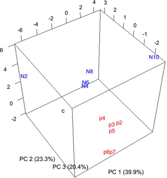
3D PCA result. The viewing angle was chosen so that the dispersion of data was the greatest. The symbols represent as follows: c, control; p2, pH 2.4; p3, pH 3.4; p4, pH 4.0; p5, pH 5.0; p6, pH 6.0; p7, pH 7.1; N2, 0.2 M NaCl; N4, 0.4 M NaCl; N6, 0.6 M NaCl; N8, 0.8 M NaCl; N10, 1.0 M NaCl.

From the biplots, metabolites that are responsible for positioning the samples in the principal component space can be readily identified. This figure can be regarded as the calibrated version of Figure 2. We can see that the control and weak NaCl stress sample are located at the upper-left quadrant while others are spread in the other quadrants in Figures 5(a) and (b). The two same samples are located in the upper-right quadrant, also separated from the rest of the samples when viewed onto the plane of PC2 and PC3 (data not shown). We can also see that the salt stress samples are spread in a much larger area than the pH stress samples. From Figures 5(a) and 5(b), we can observe that glycerol (gl), trehalose (t), and proline (P), widely known osmoprotectants, are pointing toward mild-to-medium salt stressed samples. The sample that received the strongest salt stress (1 M NaCl) is located in the opposite direction of those osmoprotectants. We speculate that this high salt pushed yeast cells over a certain limit so that the normal intracellular physiology was severely perturbed.

Figure 5.

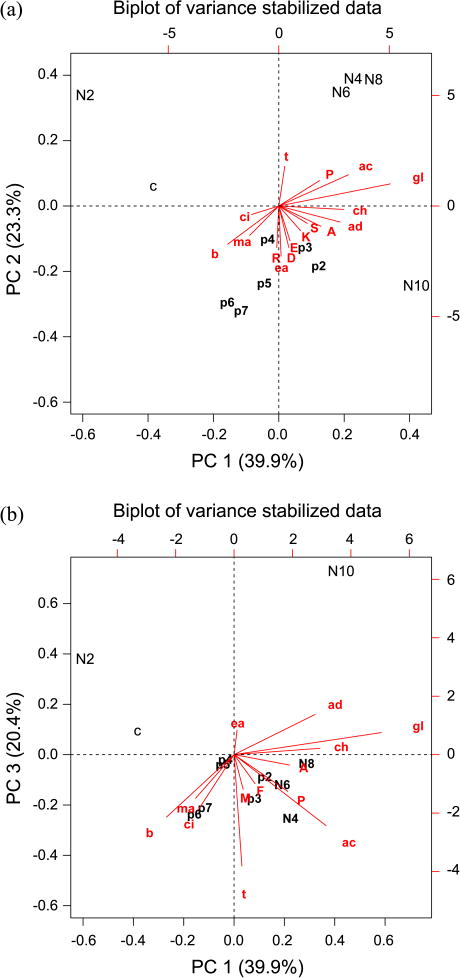
Biplots along the first and second component axes (a), and along the first and third axes (b). The symbols represent as follows: A, alanine; ac, acetate; ad, adenosine; b, betaine; ch, choline, ci, citrate; D, aspartate; E, glutamate; ea, ethanolamine; F, phenylalanine; gl, glycerol; K, lysine; M, methionine; ma, malate; P, proline; R, arginine; S, serine; t, trehalose.

Compared to NaCl stress, pH stresses were clustered together in the PCA space as shown in Figures 5(a) and 5(b). When those pH stresses were analyzed separately, they showed an interesting feature: we could observe 3 clusters: highly acidic (pH 2.4 and pH 3.4), mildly acidic (pH 4.1 and pH 5.0), and near neutral (pH 6.0 and pH 7.1) (data not shown). The key metabolites could be identified for such clustering: acetate could be regarded as a marker for highly acidic condition, ethanolamine, for a mildly acidic one, and citrate and malate, for a near neutral one. The cells seemed to cope with a mildly acidic condition by accumulating a weak base such as ethanolamine which can be converted from serine by decarboxylation. We can speculate that when pH gets low enough, cells start to accumulate acetate, which can act to trap protons sneaking from a low pH external environment. This result shows some differences from our previous work,³⁶ and we think it stems from the strain difference, that is, a different genetic background results in a different way to handle the same stress.

Conclusions

We found 31 metabolites were identified for most of the samples. The levels of many identified metabolites showed a gradual or drastic increase or decrease depending on the severity of the stress. The statistical analysis produced a holistic view: pH stresses were clustered together, but salt stresses were spread according to severity, which implicated that the latter induced more global rearrangement of the intracellular environment. This work could provide a link between the metabolite profiles and mRNA or protein profiles under representative and well studied stress conditions.

References

- 1.Devantier R, Scheithauer B, Villas-Boas SG, Pedersen S, Olsson L. Biotechnol Bioeng. 2005;90:703. doi: 10.1002/bit.20457. [DOI] [PubMed] [Google Scholar]
- 2.Ostergaard S, Olsson L, Nielsen J. Microbiol Mol Biol R. 2000;64:34. doi: 10.1128/mmbr.64.1.34-50.2000. [DOI] [PMC free article] [PubMed] [Google Scholar]
- 3.Peralta-Yahya PP, Keasling JD. Biotechnol J. 2010;5:147. doi: 10.1002/biot.200900220. [DOI] [PubMed] [Google Scholar]
- 4.Sicard D, Legras JL. C R Biol. 2011;334:229. doi: 10.1016/j.crvi.2010.12.016. [DOI] [PubMed] [Google Scholar]
- 5.Valko M, Morris H, Cronin MT. Curr Med Chem. 2005;12:1161. doi: 10.2174/0929867053764635. [DOI] [PubMed] [Google Scholar]
- 6.Gasch A. In: Yeast Stress Responses. Hohmann S, Mager W, editors. Vol. 1. Springer; Berlin/Heidelberg: 2003. p. 11. [Google Scholar]
- 7.Alexandre H, Ansanay-Galeote V, Dequin S, Blondin B. FEBS Lett. 2001;498:98. doi: 10.1016/s0014-5793(01)02503-0. [DOI] [PubMed] [Google Scholar]
- 8.Gasch AP, Spellman PT, Kao CM, Carmel-Harel O, Eisen MB, Storz G, Botstein D, Brown PO. Mol Biol Cell. 2000;11:4241. doi: 10.1091/mbc.11.12.4241. [DOI] [PMC free article] [PubMed] [Google Scholar]
- 9.Causton HC, Ren B, Koh SS, Harbison CT, Kanin E, Jennings EG, Lee TI, True HL, Lander ES, Young RA. Mol Biol Cell. 2001;12:323. doi: 10.1091/mbc.12.2.323. [DOI] [PMC free article] [PubMed] [Google Scholar]
- 10.Boy-Marcotte E, Lagniel G, Perrot M, Bussereau F, Boudsocq A, Jacquet M, Labarre J. Mol Microbiol. 1999;33:274. doi: 10.1046/j.1365-2958.1999.01467.x. [DOI] [PubMed] [Google Scholar]
- 11.Strassburg K, Walther D, Takahashi H, Kanaya S, Kopka J. Omics. 2010;14:249. doi: 10.1089/omi.2009.0107. [DOI] [PMC free article] [PubMed] [Google Scholar]
- 12.Berry DB, Gasch AP. Mol Biol Cell. 2008;19:4580. doi: 10.1091/mbc.E07-07-0680. [DOI] [PMC free article] [PubMed] [Google Scholar]
- 13.Nicholson JK, Holmes E, Lindon JC, Wilson ID. Nat Biotech. 2004;22:1268. doi: 10.1038/nbt1015. [DOI] [PubMed] [Google Scholar]
- 14.Griffin JL, Bonney SA, Mann C, Hebbachi AM, Gibbons GF, Nicholson JK, Shoulders CC, Scott J. Physiol Genomics. 2004;17:140. doi: 10.1152/physiolgenomics.00158.2003. [DOI] [PubMed] [Google Scholar]
- 15.Raamsdonk LM, Teusink B, Broadhurst D, Zhang N, Hayes A, Walsh MC, Berden JA, Brindle KM, Kell DB, Rowland JJ, Westerhoff HV, van Dam K, Oliver SG. Nat Biotechnol. 2001;19:45. doi: 10.1038/83496. [DOI] [PubMed] [Google Scholar]
- 16.Saito K, Matsuda F. Annu Rev Plant Biol. 2010;61:463. doi: 10.1146/annurev.arplant.043008.092035. [DOI] [PubMed] [Google Scholar]
- 17.Hannah MA, Caldana C, Steinhauser D, Balbo I, Fernie AR, Willmitzer L. Plant Physiol. 2010;152:2120. doi: 10.1104/pp.109.147306. [DOI] [PMC free article] [PubMed] [Google Scholar]
- 18.Daviss B. Scientist. 2005;19:25. [Google Scholar]
- 19.Jordan KW, Nordenstam J, Lauwers GY, Rothenberger DA, Alavi K, Garwood M, Cheng LL. Dis Colon Rectum. 2009;52:520. doi: 10.1007/DCR.0b013e31819c9a2c. [DOI] [PMC free article] [PubMed] [Google Scholar]
- 20.Wishart DS, Tzur D, Knox C, Eisner R, Guo AC, Young N, Cheng D, Jewell K, Arndt D, Sawhney S, Fung C, Nikolai L, Lewis M, Coutouly M-A, Forsythe I, Tang P, Shrivastava S, Jeroncic K, Stothard P, Amegbey G, Block D, Hau DD, Wagner J, Miniaci J, Clements M, Gebremedhin M, Guo N, Zhang Y, Duggan GE, MacInnis GD, Weljie AM, Dowlatabadi R, Bamforth F, Clive D, Greiner R, Li L, Marrie T, Sykes BD, Vogel HJ, Querengesser L. Nucl Acids Res. 2007;35:D521. doi: 10.1093/nar/gkl923. [DOI] [PMC free article] [PubMed] [Google Scholar]
- 21.Cui Q, Lewis IA, Hegeman AD, Anderson ME, Li J, Schulte CF, Westler WM, Eghbalnia HR, Sussman MR, Markley JL. Nat Biotechnol. 2008;26:162. doi: 10.1038/nbt0208-162. [DOI] [PubMed] [Google Scholar]
- 22.Smith CA, O’Maille G, Want EJ, Qin C, Trauger SA, Brandon TR, Custodio DE, Abagyan R, Siuzdak G. Therapeutic Drug Monitoring. 2005;27:747. doi: 10.1097/01.ftd.0000179845.53213.39. [DOI] [PubMed] [Google Scholar]
- 23.Jewison T, Knox C, Neveu V, Djoumbou Y, Guo AC, Lee J, Liu P, Mandal R, Krishnamurthy R, Sinelnikov I, Wilson M, Wishart DS. Nucleic Acids Res. 2012;40:D815. doi: 10.1093/nar/gkr916. [DOI] [PMC free article] [PubMed] [Google Scholar]
- 24.Akiyama K, Chikayama E, Yuasa H, Shimada Y, Tohge T, Shinozaki K, Hirai MY, Sakurai T, Kikuchi J, Saito K. Silico Biology. 2008;8:339. [PubMed] [Google Scholar]
- 25.Lewis IA, Schommer SC, Hodis B, Robb KA, Tonelli M, Westler WM, Sussman MR, Markley JL. Anal Chem. 2007;79:9385. doi: 10.1021/ac071583z. [DOI] [PMC free article] [PubMed] [Google Scholar]
- 26.Delaglio F, Grzesiek S, Vuister GW, Zhu G, Pfeifer J, Bax AJ. Biomol NMR. 1995;6:277. doi: 10.1007/BF00197809. [DOI] [PubMed] [Google Scholar]
- 27.Lewis IA, Schommer SC, Markley JL. Magn Reson Chem. 2009;47(Suppl 1):S123. doi: 10.1002/mrc.2526. [DOI] [PMC free article] [PubMed] [Google Scholar]
- 28.Maharjan RP, Ferenci T. Analytical Biochemistry. 2003;313:145. doi: 10.1016/s0003-2697(02)00536-5. [DOI] [PubMed] [Google Scholar]
- 29.Villas-Boas SG, Hojer-Pedersen J, Akesson M, Smedsgaard J, Nielsen J. Yeast. 2005;22:1155. doi: 10.1002/yea.1308. [DOI] [PubMed] [Google Scholar]
- 30.Faijes M, Mars AE, Smid EJ. Microb Cell Fact. 2007;6:27. doi: 10.1186/1475-2859-6-27. [DOI] [PMC free article] [PubMed] [Google Scholar]
- 31.Hiller J, Franco-Lara E, Weuster-Botz D. Biotechnol Lett. 2007;29:1169. doi: 10.1007/s10529-007-9384-8. [DOI] [PubMed] [Google Scholar]
- 32.Robinette SL, Ajredini R, Rasheed H, Zeinomar A, Schroeder FC, Dossey AT, Edison AS. Anal Chem. 2011 doi: 10.1021/ac102724x. [DOI] [PMC free article] [PubMed] [Google Scholar]
- 33.Motta A, Paris D, Melck D. Anal Chem. 2010;82:2405. doi: 10.1021/ac9026934. [DOI] [PubMed] [Google Scholar]
- 34.Martineau E, Giraudeau P, Tea I, Akoka SJ. Pharm Biomed Anal. 2011;54:252. doi: 10.1016/j.jpba.2010.07.046. [DOI] [PubMed] [Google Scholar]
- 35.Lewis IA, Schommer SC, Hodis B, Robb KA, Tonelli M, Westler WM, Suissman MR, Markley JL. Anal Chem. 2007;79:9385. doi: 10.1021/ac071583z. [DOI] [PMC free article] [PubMed] [Google Scholar]
- 36.Kang WY, Kim SH, Chae YK. FEMS Yeast Res. 2012;12:608. doi: 10.1111/j.1567-1364.2012.00811.x. [DOI] [PubMed] [Google Scholar]