

Abstract
Numerous word recognition studies conducted over the past 2 decades are examined. These studies manipulated lexical familiarity by presenting words of high versus low printed frequency and most reported an interaction between printed frequency and one of several second variables, namely, orthographic regularity, semantic concreteness, or polysemy. However, the direction of these interactions was inconsistent from study to study. Six new experiments clarify these discordant results. The first two demonstrate that words of the same low printed frequency are not always equally familiar to subjects. Instead, subjects’ ratings of “experiential familiarity” suggest that many of the low-printed-frequency words used in prior studies varied along this dimension. Four lexical decision experiments reexamine the prior findings by orthogonally manipulating lexical familiarity, as assessed by experiential familiarity ratings, with bigram frequency, semantic concreteness, and number of meanings. The results suggest that of these variables, only experiential familiarity reliably affects word recognition latencies. This in turn suggests that previous inconsistent findings are due to confounding experiential familiarity with a second variable.
Twenty years of research on word recognition has repeatedly shown that the familiarity of a word greatly affects both the speed and the accuracy of its recognition. More familiar words can be recognized faster and more accurately than less familiar words. Traditionally, lexical familiarity has been operationalized as the frequency with which a word occurs in printed English text. Experimenters typically construct their stimulus sets by consulting one of three widely used indices: Thorndike and Lorge’s (1944) Teacher’s Word Book of 30,000 Words, Kučera and Francis’s (1967) Computational Analysis of Present-Day American English, or Carroll, Davies, and Richman’s (1971) American Heritage Word Frequency Book. Within these corpora, one would find that the English word amount occurs relatively frequently (with an average frequency score of 110 occurrences per million words of text), whereas the word amour occurs relatively infrequently (with an average frequency score of 1 occurrence per million words of text).
The Effect of Printed Frequency
Howes and Solomon (1951) reported that printed frequency could account for approximately half of the variance found in tachistoscopic thresholds. Similarly, Rubenstein, Garfield, and Millikan (1970) reported that, on the average, lexical decision latency to a high-printed-frequency word is significantly shorter than that to a low-printed-frequency word, such that words that differ in printed frequency by a factor of 10 usually show a 75-ms difference in response latency. A less conservative estimate has been given by Scarborough, Cortese, and Scarborough (1977): A 50-ms difference in response time occurs between words that differ by one logarithmic unit of printed frequency. According to an average of these estimates, the word amount should be recognized a little more than 100 ms faster than the word amour.
Despite wide evidence for printed frequency’s potency in predicting both speed and accuracy in word recognition, there is little agreement about the mechanism underlying its robust effect. There appear to be two broad classes of theories. One theoretical camp supported the proposition that the effect of printed frequency was perceptual; in simplistic terms, high-printed-frequency words elicit superior recognition performance because they are more easily seen (e.g., Catlin, 1969; Newbigging, 1961; Rumelhart & Siple, 1974; Savin, 1963; Solomon & Postman, 1952). Their opponents argued that the effect of printed frequency derived from response processes: High-printed-frequency words can evoke responses more rapidly (e.g., Adams, 1979; Broadbent, 1967; Morton, 1968; Treisman, 1971).
These theories were based on the implicit assumption that high- and low-printed-frequency words are equivalent along all other relevant dimensions. But Landauer and Streeter (1973) disconfirmed this assumption. They demonstrated that the distribution of letters and phonemes differs significantly in high- and low-printed-frequency words. That is, high-printed-frequency words are likely to contain more regularly occurring phonemic and graphemic patterns than low-printed-frequency words. Landauer and Streeter’s work supported Carroll and White’s caveat: “Word frequency may not be the simple variable that it appears to be” (1973, p. 563).
To be sure, other variables do covary with printed frequency, and the effect of printed frequency may be partially attributable to these secondary variables. Besides differing in orthographic and phonemic structure, high-printed-frequency words also differ from low-printed-frequency words along semantic and lexicographic dimensions. Paivio, Yuille, and Madigan (1968) noted that a greater proportion of high-printed-frequency words are concrete or imageable rather than abstract, whereas the reverse is true of low-printed-frequency words. Furthermore, high-printed-frequency words tend to have more individual meanings (Glanzer & Bowles, 1976; Reder, Anderson, & Bjork, 1974; Schnorr & Atkinson, 1970).
In the last 20 years, many researchers have orthogonally manipulated the printed-frequency variable with these other variables in the hope of discovering the nature of the printed-frequency effect. With few exceptions, high-printed-frequency words were recognized with a consistently high level of accuracy or speed, regardless of their orthographic regularity, semantic concreteness, or number of meanings. Performance with low-printed-frequency words has not been so consistent. Rather, recognition of low-printed-frequency words has often interacted with the above three variables in paradoxical and inconsistent ways.
The Inconsistent Interaction Between Printed Frequency and Bigram Frequency
Just as English words differ in frequency of occurrence, so the components of those words, individual letters and letter patterns, differ in frequency of occurrence (Shannon, 1948). One measure of orthographic frequency is bigram frequency, that is, the frequency of two letters occurring in tandem in a particular position of a particular length word. As an illustration, the bigram WH frequently occurs as the first bigram of a five-letter word, but never as the last bigram of a five-letter word.
Orsowitz (1963, cited in Biederman, 1966) factorially combined printed frequency with bigram frequency. Subjects were tachistoscopically presented with five-letter words, and the number of trials to accurately recognize each stimulus word was recorded. Orsowitz found that the effects of printed frequency and bigram frequency were not additive but interactive and that the interaction was somewhat paradoxical. For high-printed-frequency words, bigram frequency had no effect, but for low-printed-frequency words, more trials were required to recognize words with high-frequency bigram (high-bigram words) than words with low-frequency bigrams (low-bigram words). This result was corroborated by Broadbent and Gregory (1968). Rice and Robinson (1975) also corroborated the Orsowitz results, using a lexical decision paradigm: Subjects were required to decide quickly whether letter strings composed a word. The mean reaction time (RT) and percentage of errors revealed that for high-printed-frequency words, bigram frequency had no effect, but responses to low-printed-frequency/high-bigram words were slower and less accurate than those to low-printed-frequency/low-bigram words.
Biederman (1966) tachistoscopically presented subjects with Orsowitz’s five-letter words and measured temporal threshold for accurate identification, but found opposite results. Indeed, Biederman found the usual main effect of printed frequency, but conversely found that low-printed-frequency words containing high-frequency bigrams were recognized in fewer trials than those composed of low-frequency bigrams. In a second experiment, using only low-printed-frequency words, Biederman again found an advantage for a high-bigram frequency in recognizing low-printed-frequency words. Rumelhart and Siple (1974) reported the same interaction as Biederman (1966, Experiment 1). Adding further to the puzzle, McClelland and Johnston (1977) reported no interaction. The results of these studies are summarized in Table 1.
Table 1.
Results of Studies That Have Examined the Effects of Printed Frequency and Bigram Frequency and Results of Experiment 2
| Original study | Orignal results | Results of Experiment 2 |
|---|---|---|
| Broadbent & Gregory (1968) | HBF worse than LBF | HBF less familiar than LBF |
| Rice & Robinson (1975) | HBF worse than LBF | HBF less familiar than LBF |
| Biederman (1966, Experiment 2) | HBF better than LBF | HBF more familiar than LBF |
| Biederman (1966, Experiment 1)a | HBF better than LBF | HBF equally familiar as LBF |
| Orsowitz (1963, cited in Biederman, 1966)a | HBF worse than LBF | HBF equally familiar as LBF |
| Rumelhart & Siple (1974)b | HBF better than LBF | — |
| McClelland & Johnston (1977)b | HBF same as LBF | — |
Note. Data are for low-printed-frequency words only. HBF = high bigram frequency words, LBF = low bigram frequency words.
The same stimulus words were used in these two original experiments.
Not examined in Experiment 2 because their stimuli were not available.
Though contradictory, the results of the Biederman (1966), Rumelhart and Siple (1974), and McClelland and Johnston (1977) studies are straightforward. The most puzzling finding is the paradoxical interaction reported by Orsowitz (1963, cited in Biederman, 1966), Broadbent and Gregory (1968), and Rice and Robinson (1975). It does not seem reasonable that the greater the frequency of a word’s bigrams, the worse its recognition will be.
However, an explanation has been offered: Subjects are “sophisticated guessers” (cf. Broadbent, 1967; Neisser, 1967; Newbigging, 1961; Solomon & Postman, 1952). When recognizing tachistoscopically presented words, subjects are likely to guess at a partially recognized stimulus. And presumably their guessing works against them when recognizing low-printed-frequency words composed of high-frequency bigrams. That is, with low-printed-frequency words, if the orthography resembles a high-frequency word (i.e., the word is composed of high-frequency bigrams), subjects will be likely to guess a high-frequency word, and of course, be incorrect. Sophisticated guessing is believed to be even more attractive when the low-printed-frequency words are from a very low range of printed frequency (cf. Rumelhart & Siple, 1974), or are preceded or followed by a visual mask (cf. McClelland & Johnston, 1977; McClelland & Rumelhart, 1981).
Rice and Robinson (1975) conceded that a sophisticated guessing strategy could also be operating in their lexical decision task, though their data suggest that sophisticated guessing cannot fully account for the performance they observed. The RTs from their study revealed the typical paradoxical interaction between bigram frequency and printed frequency, yet they found no effect of bigram frequency on their subjects’ performance with nonword stimuli. If the paradoxical disadvantage of high bigram frequency in low-printed-frequency words is caused by subjects’ sophisticated guessing, surely one would predict longer latencies or more errors for nonwords composed of high-frequency bigrams because they are more apt to resemble real words.
To summarize, the studies reviewed here have factorially manipulated printed frequency and bigram frequency, but their results have been inconsistent. All studies reported that high-printed-frequency words were recognized significantly better than low-printed-frequency words. Almost all reported an interaction between printed frequency and bigram frequency such that with high-printed-frequency words, there was no effect of bigram frequency. Orthographic regularity influenced the recognition of low-printed-frequency words but without a consistent pattern. In some studies, high bigram frequency facilitated the recognition of low-printed-frequency words; in others it led to poorer performance.
The favored explanation for the paradoxical interaction or its absence has been sophisticated guessing. Subjects dealing with inadequate visual information or under time pressure are more likely to incorrectly report or to delay responding to low-printed-frequency words composed of letter patterns that occur frequently. The purpose of Experiment 1 was to test this explanation. If the paradoxical interaction is caused by a sophisticated guessing strategy, and this strategy is induced by processing incomplete information due to brief exposure or speeded decision making, removing these inducements should eliminate the paradoxical interaction. There would be no need for sophisticated guessing if the stimuli are available for as long as subjects wish and the responses are not time pressured. Thus, subjects in Experiment 1 were presented with the stimulus words used in the Rice and Robinson (1975) study and were asked to give an unspeeded judgment of their confidence concerning the lexical status of each word.
Experiment 1
Method
Subjects
Subjects were 45 native English speakers at the University of Texas at Austin who were enrolled in an introductory psychology course and who participated in the experiment to fulfill a course requirement.
Materials
The materials were the 60 words and 60 nonwords used by Rice and Robinson (1975). Half of the 60 real words occurred frequently in printed material; half occurred infrequently. Half of each frequency set contained high-frequency bigrams, the other half, low-frequency bigrams. In addition, half of the nonwords contained high-frequency bigrams, and the other half, low-frequency bigrams.
The 120 words and nonwords were randomly arranged and typed on five pages, 24 words to a page, with the constraints that no more than 2 words or nonwords appeared consecutively and that an equal number of items from each of the original six conditions appeared on a page. The words, typed in capitals, appeared down the left-hand margin. Opposite each word was a 7-point numerical scale, with its ends labeled HIGHLY CONFIDENT IS NOT A WORD and HIGHLY CONFIDENT IS A WORD. The order of the five pages was randomized for each set, and the pages were collated into a booklet that included a cover sheet with written instructions and a space for name, session number, and date.
Procedure
Subjects were asked to rate their confidence concerning the lexical status of letter strings. Specific instructions were read silently by each subject while the experimenter read them aloud at the beginning of the experimental session. These instructions encouraged subjects to work at their own rate and to “please take as much time to make each decision as needed.”
Results and Discussion
Mean ratings were computed for each item by averaging across all subjects’ responses to a given item. A 2 × 2 (Printed Frequency × Bigram Frequency) analysis of variance (ANOVA) was performed on the ratings for the word stimuli. This analysis revealed a significant main effect of printed frequency, F(1, 56) = 54.00, p < .001, a main effect of bigram frequency, F(1, 56) = 6.41, p < .01, and a significant interaction between the two variables, F(1, 56) = 5.40, p < .02. Figure 1 compares the mean lexical confidence ratings for the four word conditions with the mean RT obtained to these same items by Rice and Robinson (1975). Bigram frequency affected lexical confidence only for the low-printed-frequency words. For high-printed-frequency words, the mean lexical confidence rating for words with high-frequency bigrams (M = 6.6) did not differ significantly from the ratings for words with low-frequency bigrams (M = 6.6), t(28) = 0.33, p > .70. For low-printed-frequency words, subjects were less confident that Rice and Robinson’s high-bigram words (M = 5.6) were real words than that their low-bigram words (M = 6.1) were, t(28) = 2.56, p < .02. This pattern mirrored the latency data reported by Rice and Robinson. Percentage response to the top of the confidence scale reveals these effects more dramatically. To the high-printed-frequency/high-bigram words, 90% of the subjects responded HIGHLY CONFIDENT IS A WORD, compared with 89% to the high-printed-frequency/low-bigram words. In response to the low-printed-frequency words, 63% of the subjects responded HIGHLY CONFIDENT IS A WORD to those composed of low-frequency bigrams, compared with 45% to those composed of high-frequency bigrams, t(28) = 2.29, p < .03.
Figure 1.
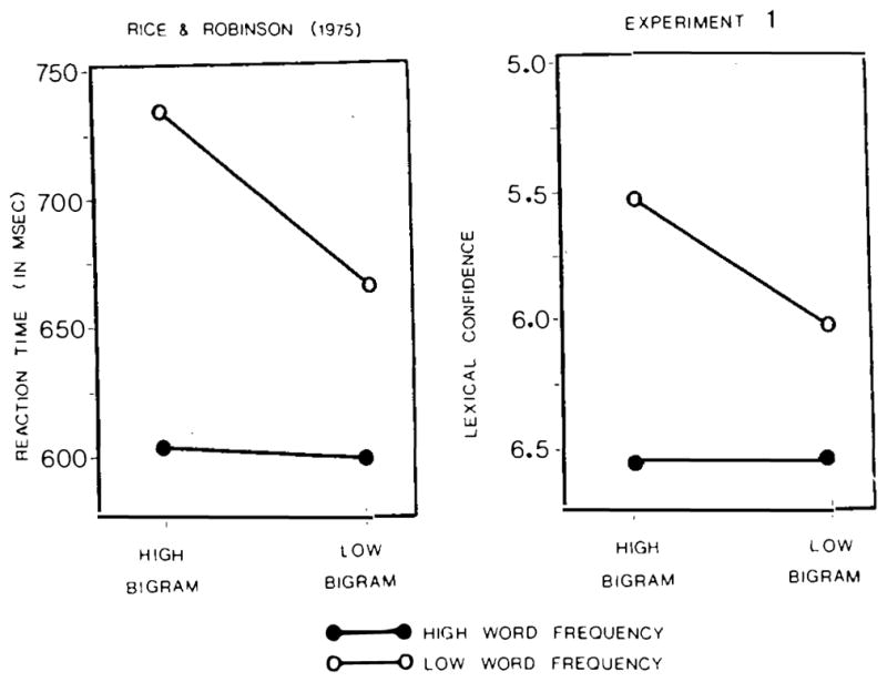
Mean reaction time from Rice and Robinson’s (1975) study and mean lexical confidence ratings from Experiment 1 for word stimuli.
This paradoxical interaction between bigram frequency and printed frequency seriously challenges the sophisticated guessing explanation of this result. The present subjects, unlike those in Rice and Robinson’s (1975) experiment, performed the task without any speed pressure. Moreover, the stimulus words were not presented briefly, as in the Orsowitz (1963, cited in Biederman, 1966) and Broadbent and Gregory (1968) studies, nor were they visually masked, as in the McClelland and Johnston (1977) study, and they were in the same frequency range as those in the Biederman (1966) study. The only procedure common to all these studies was the presentation of high- and low-printed-frequency words that differed in bigram frequency. Even more striking, the present study and that by Rice and Robinson (1975) used the same words. Thus, the source of this 20-year discrepancy may reside in the stimulus words themselves.
The Reliability of Printed Frequency
A potential problem of counts of printed frequency is that they are, by definition, based on literary samples of word usage. For example, the word comma occurs only once or twice per million words of text, but the word chapter occurs 50 to 100 times. It is doubtful that chapter is 50 to 100 times more familiar than comma. Consider also the changes in contemporary English usage since printed frequency counts were first assembled. Only a few years after the Thorndike and Lorge (1944) count was published, Howes (1954) questioned, “to what extent can word frequencies based on the linguistic behavior of writers in the 1930’s represent the average base probabilities of Harvard students in 1948?” (p. 106). The problem must be more serious in the 1980s, yet in psycholinguistic research published from 1970 to the present, the older Thorndike and Lorge count was still favored over the newer Kučera and Francis (1967) count by approximately 2 to 1 (White, 1983). (The Carroll et al., 1971, count was based on grade school literature and is rarely used in experiments with adult subjects.)
Another problem with counts of printed frequency is that they are, by definition, samples and so are subject to sampling error. Low-printed-frequency words are subject to the greatest sampling bias (Carroll, 1967, 1970), both in the original collection of the corpora and in the subsequent selection by experimenters. For example, consider the words, boxer, icing, and joker as opposed to loire, gnome, and assay. Intuitively, it seems the words in the first set would be familiar to most college undergraduates, whereas those in the second would be unfamiliar. Yet both groups of words have frequency scores of 1 in both the Thorndike and Lorge (1944) and Kučera and Francis (1967) counts.
A second sampling error can occur when low-printed-frequency words are selected for material sets that manipulate other properties of the stimulus words. For example, Rice and Robinson (1975) selected two groups of low-printed-frequency words, each occurring once per million and hence matched for printed frequency. One group was composed of words such as fumble, mumble, giggle, drowsy, snoop, and lava. A second group contained words such as cohere, heron, rend, char, cant, and pithy. The words in the first group comprised low-frequency bigrams; the words in the second comprised high-frequency bigrams. Rice and Robinson found slower RTs to words in the second group and concluded that high bigram frequency interfered with recognition of low-printed-frequency words.
Another explanation may be that the words in the first set are simply more familiar. Gernsbacher (1983) had subjects rate their subjective, termed “experiential,” familiarity with 455 low-printed-frequency words. The reliability of these ratings was high; different raters agreed closely. More important, the range of ratings was broad and well distributed, suggesting that words with the same low-printed-frequency score can differ substantially in their experiential familiarity.
A difference in the experiential familiarity of the stimulus words used in previous studies could explain not only the paradoxical interaction between printed frequency and bigram frequency but also the reverse interaction or even the absence of an interaction. That is, given the sampling error that may occur with printed frequency counts, the probability of confounding experiential familiarity with bigram frequency would be most likely to occur in words selected from the low-printed-frequency range. Studies reporting that low-printed-frequency/low-bigram words were better recognized might have used low-printed-frequency/low-bigram words that were more familiar than their low-printed-frequency/high-bigram counterparts. Studies reporting a significant interaction in the opposite direction might have used materials with an opposite confound. Studies reporting no interaction probably avoided the confound. To test this possibility, a measure of the experiential familiarity of the low-printed-frequency words used in those studies was needed.
Experiment 2
Method
Subjects
Subjects were 44 native English speakers at the University of Texas at Austin who were enrolled in an introductory psychology course and who participated in the experiment to fulfill a course requirement. Data from an additional subject were excluded because he failed to perform the task carefully, as indicated by his responses to the catch words.
Materials
The experimental set of words comprised all the low-printed-frequency words from the materials used by Orsowitz (1963, cited in Biederman, 1966), Biederman (1966), Broadbent and Gregory (1968), and Rice and Robinson (1975), and 40 low-printed-frequency words used in a study by Rubenstein et al. (1970). Thus the experimental set consisted of 42 low-printed-frequency words composed of high-frequency bigrams and 42 low-printed-frequency words composed of low-frequency bigrams taken from four of the studies reviewed earlier, as well as 40 low-printed-frequency words from the Rubenstein et al. (1970) stimuli. In addition to the 124 words from the five previous studies. 7 five-letter words of high (AA) printed frequency were added as a check for the validity of individual subject’s rating. As a second validity measure, 7 five-letter nonwords, which conformed to the rules of English orthography, were constructed and added to the stimulus list. An additional 37 low-printed-frequency words, which matched the average letter length of the experimental words, were selected as filler words.
All 175 words were randomly arranged and typed on seven pages, 25 words to a page, with the constraint that no more than one of either type “control” (i.e., AA or nonword) word appeared on a page. The words, typed in capitals, appeared down the left-hand margin. Opposite each word was a 7-point numerical scale, with its ends labeled VERY UNFAMILIAR and VERY FAMILIAR. The order of the seven pages was randomized, and the pages were collated into a booklet that included a cover sheet with written instructions.
Procedure
Subjects rated how familiar they were with each word on the list. Specific instructions were read silently by each subject while the experimenter read them aloud. Subjects were then encouraged to work at their own rate.
Results and Discussion
Sums were computed for each word at each level of the 7-point scale. Two subjects failed to respond to every item in their booklets; therefore, sums were converted to proportions by dividing the total number of responses for a given level by the total number of subjects responding to that item. Mean proportions were tabulated for the words within each original condition of a previous study. The results of this experiment are compared with those of the original studies in Table 1.
Broadbent and Gregory (1968) and Rice and Robinson (1975) reported that low-printed-frequency words composed of low-frequency bigrams were better recognized than low-printed-frequency words composed of high-frequency bigrams. Experiment 2 revealed that the low-printed-frequency/low-bigram words used by Broadbent and Gregory were rated as VERY FAMILIAR by 74.33% of the present subjects, whereas their low-printed-frequency/high-bigram words were rated as VERY FAMILIAR by only 46.07% of these subjects, t(28) = 3.50, p < .001. In addition, the low-printed-frequency/low-bigram words used by Rice and Robinson were rated as VERY FAMILIAR by more subjects (96%) than the low-printed frequency/high-bigram words (74%) used in that study, t(28) = 3.09, p < .001.
Biederman (1966, Experiment 2) reported the opposite effect, namely, that low-printed-frequency words composed of high-frequency bigrams were recognized better than low-printed-frequency words composed of low-frequency bigrams. His low-printed-frequency/high-bigram words were rated as VERY FAMILIAR by 50.13% of the subjects in the present study, whereas his low-printed-frequency/low-bigram words were rated as VERY FAMILIAR by only 29.57% of these subjects. However, perhaps because there were only eight words per cell, this 20% difference in mean ratings is only marginally significant at a conservative level, t(14) = 1.38, p < .091. Yet, when the familiarity data for the Biederman high-bigram stimuli are added to those generated by the Broadbent and Gregory (1968) low-bigram stimuli, and when the Biederman low-bigram stimuli are added to the Broadbent and Gregory high-bigram stimuli, the combined test is highly significant, t(44) = 3.41, p < .001.
Finally, Orsowitz (1963, cited in Biederman, 1966) reported a bigram frequency disadvantage, whereas Biederman (1966, Experiment 1), using the exact same stimuli, reported the exact opposite finding, a bigram frequency advantage. The results of the familiarity ratings obtained for the original Orsowitz stimuli are equivocal. In the present experiment, Orsowitz’s high-bigram words were rated as VERY FAMILIAR by 31.25% of the subjects; the low-bigram words were rated as VERY FAMILIAR by 28.00% of the subjects. This difference is not statistically significant.
To summarize, the low-printed-frequency words used in some previous experiments apparently differ in their rated experiential familiarity. Irrespective of orthographic frequency, the mean levels of experiential familiarity found in Experiment 2 could easily account for many of the observed interactions with low printed frequency reported in the original experiments. Furthermore, experiential familiarity might well account for artifactual differences in other experiments, since the present experiment investigated only studies in which authors had published their stimuli.
The purpose of Experiment 3 was to examine this hypothesis more directly. As previously mentioned, Gernsbacher (1983) obtained experiential familiarity scores for all five-letter words indexed by Thorndike and Lorge (1944) occurring once per million. The stimulus words were drawn from this corpus. In Experiment 3, subjects made lexical decisions to words that were factorial arrangements of experiential familiarity and bigram frequency, each at two levels. It was expected that lexical decisions to words with high experiential familiarity would be faster than to words with low experiential familiarity, but that no effect of or interaction with bigram frequency would result.
Experiment 3
Method
Subjects
The subjects in this and the subsequent three experiments were drawn from the same population of those who had generated the familiarity ratings (Gernsbacher, 1983), and all were native English speakers. No subject who had served in the original rating experiment served in any of the present experiments, nor did any subject serve in more than one experiment. The subjects in Experiment 3 were 19 undergraduate students enrolled in introductory psychology at the University of Texas at Austin, who participated to fulfill a course requirement. The data from 3 additional subjects were excluded because they performed below the a priori error criterion of no more than 30% errors in any one of the six experimental conditions.
Design and materials
Four groups of 20 five-letter words were selected from the aforementioned corpus. One group consisted of words that were rated as VERY FAMILIAR by at least 75% of the subject raters and that comprised high-frequency bigrams. A second group consisted of words that were also rated as VERY FAMILIAR by at least 75% of the raters but that comprised low-frequency bigrams. A third group consisted of words that were rated as VERY FAMILIAR by no more than 15% of the raters and that comprised high-frequency bigrams. The last group consisted of words that were rated as VERY FAMILIAR by no more than 15% of the raters and that comprised low-frequency bigrams. The bigram frequencies were obtained from the data presented by Massaro, Taylor, Venezky, Jastrzembski, and Lucas (1980). The mean summed bigram frequency was 8,395 for the high-familiarity/high-bigram words, 1,069 for the high-familiarity/low-bigram words, 8,340 for the low-familiarity/high-bigram words, and 1,029 for the low-familiarity/low-bigram words. (Units for the bigram frequency scores are the number of occurrences per million words for each of the four bigrams in a five-letter word. These are summed and positional.)
The nonword stimuli were constructed in the same way as those of Rice and Robinson (1975). Five-letter nonwords were generated by a computer program that selected letter pairs according to their bigram frequency. By this method, the nonwords were first-order approximations to English words. Nonlexicality in this and all subsequent experiments was defined as failure to appear in the unabridged Webster’s New World Dictionary (1981). In addition, nonwords that contained embedded real words of three letters or more were not used. Forty nonwords were selected to match the mean of the high-bigram word stimuli, collapsed over familiarity. The mean bigram frequency of these nonwords was 8,358. Another 40 nonwords were selected to match the mean of the word items with low bigram frequency. The mean bigram frequency of these nonwords was 1,040. The experiment was therefore a 3 × 2 (Word Type × Bigram Frequency) design, with both variables manipulated within subjects.
Apparatus and procedure
The experiment was controlled by a Digital Equipment Corporation PDP-11/03, which was responsible for stimulus randomization, stimulus presentation, and data collection. The five-letter strings were displayed in uppercase white Matrox letters on the black background of a Setchell Carlson television screen. Two subjects were tested in each experimental session, with subjects occupying separate booths and the experimenter monitoring the session from an adjacent room. Subjects were seated approximately 3 ft (0.9144 m) in front of the television screen. A stimulus trial consisted of the presentation of a warning dot in the center of the television screen, appearing coincident with a short warning tone and followed 500 ms later by the stimulus item. A millisecond timer was activated coincidentally with the presentation of the stimulus item. The stimulus item remained in view until subjects in both booths had responded. One second elapsed between the removal of a stimulus item and the presentation of the warning dot and tone of the next trial.
Subjects were informed of the sequence of events for each stimulus trial. They were told that they would be shown groups of letters and that their task was to decide whether the letters formed a real word in English. All subjects used the index finger of their preferred hand to indicate “yes” and the index finger of their nonpreferred hand to indicate “no.” Subjects were informed that approximately half of the letter groups would indeed form real words and half would not and that some of the real words presented might be slightly unfamiliar to them. Further instructions stressed speed as well as accuracy. The experimenter answered any questions about the task; subjects were given 10 practice trials, which included at least one stimulus item characteristic of each of the six stimulus conditions, and then subjects were presented with the experimental materials.
Results and Discussion
For correct RTs, a mean and standard deviation were computed for each subject and for each item in the experiment. Any individual RT that was more than 2.5 SD away from both the mean performance for the subject in that condition and the mean RT to the item across subjects was replaced, following the procedure suggested by Winer (1971). Subjects’ mean RTs and percentage of errors for each of the six experimental conditions are shown in Table 2. All ANOVAs conducted on mean RTs were also conducted on mean percentage of errors, and no discrepancies were found between the two sets of results. Therefore, only the results of the ANOVAs performed on mean RT are reported.
Table 2.
Mean Reaction Time (RT) and Percentage of Errors in Experiment 3
| Bigram frequency | High familiarity
|
Low familiarity
|
Nonword
|
|||
|---|---|---|---|---|---|---|
| RT (ms) | Errors (%) | RT (ms) | Errors (%) | RT (ms) | Errors (%) | |
| High | 719 | 2 | 970 | 19 | 1,041 | 8 |
| Low | 738 | 1 | 993 | 23 | 954 | 4 |
The mean RTs of the 19 subjects and the 160 stimulus items were both submitted to a 3 × 2 (Word Type × Bigram Frequency) ANOVA. In one analysis, subjects were treated as random effects; in a second, items were treated as random effects (Clark, 1973). In addition, the item analyses of all three levels of familiarity included a statistical procedure for unequal cell sizes. These ANOVAS revealed a significant main effect of experiential familiarity in both the analysis by subjects, F1(2, 36) = 25.02, p < .001, and the analysis by items, F2(2, 157) = 41.81, p < .001; , p < .001. As can be seen in Table 2, high-familiarity/low-printed-frequency words were recognized more than 250 ms faster than those rated as less familiar yet of equal frequency of occurrence in printed English.
The 3 × 2 ANOVA, with subjects as random effects, also revealed a main effect of bigram frequency, F1(1, 18) = 9.18, p < .007, and an interaction between experiential familiarity and bigram frequency, F1(2, 36) = 8.55, p < .001. However, these last two effects failed to reach a conservative level of significance in the analysis in which items were considered random effects, F2(1, 154) = 3.13, p < .079, and F2(2, 154) = 2.43, p < .092. Inspection of the six conditions’ means revealed that the difference in RT to high and low bigram frequency was only 19 ms in the high-familiarity conditions. For the low-familiarity items, this difference was only 23 ms. The greatest difference between high and low bigram frequency (87 ms) occurred with the nonword stimuli. Therefore, planned comparisons were performed separately on the data from the word and the nonword conditions. These planned comparisons revealed that the effect of bigram frequency was significant only in the nonword condition, F1(1, 18) = 21.42, p < .001; F2(1, 78) = 8.67, p < .004; , p < .025. In contrast, in the word conditions, bigram frequency was not significant (F1 < 1.0, F2 < 1.0), nor was the interaction between experiential familiarity and bigram frequency, F1(1, 18) = 2.70; F2(1, 76) = 1.22; all ps > .10.
Two regression analyses clarify the effects of experiential familiarity and bigram frequency in the word data. In the first, combinations of the two independent variables, the mean familiarity rating (percentage of raters responding VERY FAMILIAR) and the summed bigram frequency, were used to predict mean correct RT. In the second, the total error rate for each stimulus word was the criterion variable; the two predictor variables were the same. These analyses revealed that rated familiarity accounted for more than 55% of the variance found in the RT data, F(1, 78) = 98.01, p < .001, and for approximately 44% of the variance found in the corresponding error data, F(1, 78) = 61.36, p < .001. Conversely, bigram frequency explained only an additional 0.3% of the variance found in either measure, and entrance of this variable into either regression equation was not statistically warranted (F < 1.0). All these analyses show that lexical familiarity, operationalized as experiential familiarity, is the more critical variable affecting the speed and accuracy of recognizing an English word.
Although bigram frequency did not affect the recognition of real words, it did significantly affect the recognition of nonwords. An examination of the nonwords used in both the Rice and Robinson (1975) study and the present Experiment 3 revealed that nonwords generated by a computer program, though they might be first-order approximations to English, differ in pronounceability. In a critical study, Rubenstein, Lewis, and Rubenstein (1971a; see also Rubenstein, Richter, & Kay, 1975) demonstrated that within a lexical decision task, pronounceable nonwords are harder to reject as nonwords than are unpronounceable ones. Thus, in Experiment 3, it might have been the pronounceability rather than the bigram frequency that affected performance.
To examine this possibility, the nonword stimuli were first classified by two independent judges as pronounceable or unpronounceable. Their decisions agreed closely (r = .982). The mean RTs and mean percentage of errors to the nonwords were then analyzed by a one-way ANOVA, with the independent variable of pronounceability. The between-group difference found in both analyses was statistically significant: for the RT data, F(1, 78) = 20.24, p < .001; for the error data, F(1, 78) = 11.51, p < .001. A post hoc analysis verified that the mean RT to the pronounceable nonwords (1,078 ms) was significantly greater than that to the unpronounceable nonwords (925 ms), t(62) = 4.41, p < .001, and that the mean error rate to the pronounceable nonwords (2.26%) was significantly higher than that to the unpronounceable nonwords (1.47%), t(62) = 3.31, p < .001. In addition, regression analyses indicated that pronounceability independently accounted for 20% of the variance in RTs, F(1, 78) = 20.24, p < .001, and for 15% of the variance in error rate, F(1, 78) = 11.51, p < .001. Bigram frequency was a weaker independent predictor: It accounted for 10% of the RT variance, F(1, 78) = 9.04, p < .01, and 6% of the error rate variance, F(1, 78) = 4.97, p < .03. When added to the regression on pronounceability, bigram frequency predicted only an additional 5% of the RT variance, F(1, 77) = 5.24, p < .03, and an insignificant 3% of the error rate variance, F(1, 77) = 2.56, p > .10.
These results seem to suggest that pronounceability, as opposed to bigram frequency, was responsible for the main effect of bigram frequency revealed in the nonword data, but caution is needed here. Massaro, Venezky, and Taylor (1979a, 1979b) noted that pronounceability is so often correlated with bigram frequency, as well as single-letter frequency, that it is difficult to separate the independent contribution of either measure of orthographic structure (cf. Krueger, 1979; Mason, 1975). Experiment 4 was conducted to investigate this question. Experiment 4 was a replication of Experiment 3, without the question of pronounceability interfering with interpreting any possible bigram effect. Subjects were presented with the same real words as those in Experiment 3. However, in order to control for the possible confounding of pronounceability and bigram frequency in the nonwords, all nonwords presented in Experiment 4 were unpronounceable.
Experiment 4
Method
Subjects
The subjects were 18 undergraduate students enrolled in introductory psychology at the University of Texas at Austin. They participated to fulfill a course requirement. Data from 2 additional subjects were excluded because they performed below the a priori error criterion.
Design and materials
The real word stimuli used in Experiment 3 were used again in Experiment 4. Again, of the 80 five-letter words, 20 were high-familiarity/high-bigram words, 20 were high-familiarity/low-bigram words, 20 were low-familiarity/high-bigram words, and 20 were low-familiarity/low-bigram words. The nonword stimuli consisted of the 34 nonwords used in Experiment 3 that had been rated as unpronounceable and an additional 46 nonwords chosen from a pool of five-letter strings generated by a computer program. These additional nonwords were similarly rated by two independent judges, and only those unanimously judged as being unpronounceable were retained. The mean summed bigram frequencies for the two sets of nonwords were 8,340 for the 40 high-bigram nonwords and 1,020 for the 40 low-bigram nonwords.
Apparatus and procedure
The apparatus and procedure were identical to those used in Experiment 3.
Results and Discussion
Correct RTs were edited in the same manner as in Experiment 3, and all ANOVAs conducted on mean RTs were also conducted on mean percentage of errors. No discrepancies were revealed between the two sets of results, and so only the mean RT results are reported.
The mean RTs of the six experimental conditions are presented in Table 3. A 2 × 2 ANOVA on the responses to the real words revealed a strong main effect of experiential familiarity, F1(1, 17) = 165.43, p < .001; F2(1, 76) = 45.35, p < .001; , p < .001. As in Experiment 3, high-familiarity words were recognized more rapidly than low-familiarity words. Bigram frequency had no significant main effect, nor did it interact with experiential familiarity: for main effect, F1(1, 17) = 3.78, F2(1, 76) = 2.68; for interaction, F1(1, 17) = 3.15, F2(1, 76) = 2.28; all ps > .10. The analyses of the nonword data also failed to reveal a main effect of bigram frequency, F1(1, 17) = 2.68; F2(1, 76) = 1.08; both ps > .10.
Table 3.
Mean Reaction Time (RT) and Percentage of Errors in Experiment 4
| Bigram frequency | High familiarity
|
Low familiarity
|
Non word
|
|||
|---|---|---|---|---|---|---|
| RT (ms) | Errors (%) | RT (ms) | Errors (%) | RT (ms) | Errors (%) | |
| High | 683 | 1 | 763 | 12 | 784 | 4 |
| Low | 700 | 2 | 779 | 15 | 768 | 3 |
The failure of the bigram frequency variable to significantly affect response latencies in either the word or nonword conditions supports the hypothesis that the effect of bigram frequency in the nonword condition of Experiment 3 was simply due to a failure to control for pronounceability across the high- and low-bigram conditions. Moreover, the lack of a significant effect of bigram frequency and, more important, the lack of an interaction of bigram frequency with the familiarity variable support the hypothesis that the interaction between bigram frequency and printed frequency found in previous studies was due to a failure to control for the experiential familiarity of their low-printed-frequency words. Taken together, the results of Experiments 3 and 4 strongly suggest that bigram frequency has often been confounded with experiential familiarity. This in turn has led to the inconsistent findings of an interaction between the two variables.
The Inconsistent Interaction Between Printed Frequency and Semantic Concreteness
Another variable that covaries with printed frequency is semantic concreteness. Words referring to concrete or tangible items have a higher probability of occurring in printed text than words referring to abstract or intangible items (Glanzer & Bowles, 1976; Paivio et al. 1968). During the past decade or two, researchers have examined the effects of printed frequency and semantic concreteness on word recognition. Like the experiments investigating the effects of printed frequency and orthography, the results of the experiments manipulating printed frequency and semantic concreteness have been inconsistent. Table 4 provides a summary of these results.
Table 4.
Results of Studies That Have Examined the Effects of Printed Frequency and Semantic Concreteness
| Original study | Results |
|---|---|
| Winnick & Kressel (1965) | Concrete worse than abstract |
| Paivio & O’Neill (1970) | Concrete worse than abstract |
| Richards (1976, Experiment 1) | Concrete better than abstract |
| James (1975) | |
| Experiment 1 | Concrete better than abstract |
| Experiment 2 | Concrete better than abstract |
| Experiment 3 | Concrete equal to abstract |
| Experiment 4 | Concrete equal to abstract |
| Rubenstein, Garfield, & Millikan (1970) | Concrete equal to abstract |
| Richards (1976, Experiment 2) | Concrete equal to abstract |
Note. Data are for low-printed-frequency words only.
Winnick and Kressel (1965) found a significant main effect of printed frequency but no main effect of semantic concreteness on tachistoscopic thresholds. However, there was a marginally significant interaction: Concrete low-printed-frequency words took longer to recognize than abstract low-printed-frequency words. Paivio and O’Neill (1970) also corroborated the well-established finding that high-printed-frequency words were recognized in fewer trials. In addition, their subjects required significantly more trials to recognize semantically concrete words than semantically abstract words; this difference was exaggerated in subjects’ performance with the low-printed-frequency words.
Richards (1976) reported the results of two similar experiments. The temporal threshold data of the first also indicated a main effect for printed frequency, no main effect of semantic concreteness, and a significant interaction between the two. However, the direction of the interaction in Richards’s study was different from that in Winnick and Kressel’s (1965) and Paivio and O’Neill’s (1970): For concrete words, thresholds declined systematically as a function of printed frequency, but for abstract words they did not. In a second experiment, Richards found main effects for printed frequency and concreteness. But unlike in his first experiment, none of the interactions between printed frequency and concreteness were significant. Richards explained the inconsistency by pointing out that in his first experiment, only 2 concrete words and 2 abstract words were presented at each of eight levels of printed frequency. In contrast, in the second experiment, 16 and 9 words were presented at each of two or three levels. Richards concluded that the results of his first experiment were possibly artifactual, whereas those of his second were not.
Rubenstein et al. (1970) provided a third pattern of results. In that study, lexical decision RTs indicated a main effect of printed frequency, no main effect of concreteness, and no interaction. And four experiments by James (1975) provided an even broader spectrum of results. James’s first experiment revealed no main effect of concreteness but did show a significant interaction mirroring the interactions discovered by Richards (1976). The second experiment revealed the same interaction, as well as a main effect of concreteness. Conversely, the third and fourth experiments revealed neither a significant interaction nor a main effect of concreteness.
James (1975) attributed these results to the differential levels of processing required by the demands of his paradigm: the lexical decision task. James (1975) likened responding in a lexical decision task to searching for a word in a dictionary. In some experimental situations, merely locating a lexical entry, what James termed “lexical processing,” is sufficient for making a response. In other situations, a deeper level of processing, what James termed “semantic processing,” might be required. In his dictionary analogy, this deeper semantic processing was likened to going a step beyond merely locating the desired entry to perhaps “reading” the appropriate definition of the target word. Deep semantic processing should take longer than the more superficial lexical processing and this should be reflected in longer latencies.
James (1975) proposed that in his four experiments he had manipulated depth of processing by varying the familiarity of the stimulus words and the type of catch trials (the nonwords). With highly familiar words, operationalized as high-printed-frequency words, little or no semantic processing should be required, only lexical processing. In contrast, with low-printed-frequency words, deeper semantic processing should be required because merely locating a lexical entry is insufficient for discriminating a low-printed-frequency word from a highly similar nonword distractor.
However, according to James (1975), processing need not be at the deeper level even for low-printed-frequency words when the nonwords are unpronounceable and thus extremely dissimilar to the target words. In his third experiment, unlike in his first two, he had used unpronounceable nonwords. In his fourth experiment, he used a preexperiment familiarization task (subjects were presented with each word, were asked to create a sentence using it, and were supplied with a definition of any word they claimed was unfamiliar). The familiarization task was assumed to have the effect of “temporarily raising the subjective frequency” (p. 134) of the real words. Accordingly, James surmised that the optimal level of processing need not extend past the more superficial lexical processing; thus no effect of nor interaction with the semantic concreteness variable would be realized.
Yet, the theoretical framework proposed by James (1975) only partially explains his results. The notion that additional semantic processing is required for the low-printed-frequency words accounts for the main effect of printed frequency found in all four experiments but cannot account for an interaction between printed frequency and semantic concreteness, much less a main effect of the latter variable. That is, his theory lacks a rationale for why semantic processing of abstract words should take longer than that of concrete words. Even granting that low-printed-frequency words require deeper semantic processing, why should the abstract meanings of these low-printed-frequency words be more difficult to “read” than the concrete meanings?
Furthermore, the levels-of-processing framework posited by James (1975) is insufficient in accounting for the results reported by Winnick and Kressel (1965) and Paivio and O’Neill (1970). Both studies reported that recognition performance with low-printed-frequency/concrete words differed from that with low-printed-frequency/abstract words; but neither study presented pronounceable nonwords nor nonwords of any type. Moreover, in James’s terminology, both found that concrete meanings of low-printed-frequency words were more difficult to “read” than abstract meanings.
To summarize, all of the studies reviewed in this section have factorially manipulated printed frequency and semantic concreteness. Their results have been inconsistent. Many experimenters have reported an interaction between the two variables, but neither this interaction nor its direction has been replicated across all experiments, even those performed by the same experimenter.
The source of these inconsistent interactions could be the same as the source of the inconsistent interactions between printed frequency and bigram frequency: the inadequacy of printed frequency counts in reflecting experiential familiarity. Direct evidence that experiential familiarity has been confounded with semantic concreteness was found in post hoc analyses conducted by Paivio and O’Neill (1970). They too questioned the reliability of printed frequency and so they obtained ratings of subjective familiarity for each of their stimulus words. Rated familiarity correlated strongly with both the concreteness values and the recognition scores. When rated familiarity was partialed out, the correlation between the concreteness values and recognition scores dropped dramatically to zero.
Other studies reviewed in this section might also have been flawed by relying on printed frequency as a reliable index of lexical familiarity, and their results might be better attributed to experiential familiarity than semantic concreteness. Experiment 5 was intended to test this possibility. In order to manipulate lexical familiarity, the stimulus words used in Experiment 5 were also selected from the rated, low-printed-frequency words collected by Gernsbacher (1983). Experiment 5 also directly tested James’s (1975) assertions concerning the differential effects of nonword pronounceability in a lexical decision task.
Experiment 5
Method
Subjects
The subjects were 20 undergraduate students at the University of Texas at Austin, enrolled in introductory psychology, who participated in the experiment to fulfill a course requirement. Eleven subjects were randomly assigned to the unpronounceable nonword condition; 9 were assigned to the pronounceable nonword condition. Data from two additional subjects in the pronounceable condition were excluded: One subject failed to perform above the a priori error criterion, and the other subject’s mean latencies, in all conditions, were well above 2.5 s.
Design and materials
The word stimuli were selected from the aforementioned corpus of low-printed-frequency, five-letter words. The selection of abstract as opposed to concrete nouns was accomplished in the following manner. Two independent judges were given 125 high-familiarity nouns, namely, all the nouns to which 50%–93% of the raters had responded VERY FAMILIAR, and 125 low-familiarity nouns, namely, all the nouns to which only 7%–20% of the raters had responded VERY FAMILIAR. From each of these two lists, the judges were instructed to select 40 nouns that “specifically referred to a tangible object, person or thing” and 40 nouns that “primarily referred to an intangible person, object or thing.” The judges were supplied with the definition of each noun, taken from Webster’s New Collegiate Dictionary (1976), to aid them in their decision. From these four lists of 40 nouns each, four experimental groups of 20 nouns each were selected by factorially combining high and low familiarity with semantic abstraction and concreteness. This selection was made with the constraints that each stimulus noun must have appeared on both judges’ lists and that across the concrete or abstract conditions, the noun sets were matched for mean familiarity ratings. The mean familiarity ratings for the high-familiarity, semantically concrete or semantically abstract nouns were 64.55% and 64.30%, respectively; the mean familiarity ratings for the low-familiarity, semantically concrete or semantically abstract nouns were 13.32% and 13.68%, respectively.
The nonword stimuli were selected from a pool generated by a computer program that produced second-order approximations to real English words. Eighty nonwords were selected that were unpronounceable, and 80 nonwords were selected that conformed to English pronunciation rules. Both groups of nonwords were matched for their summed positional bigram frequency: The means of the unpronounceable and pronounceable nonwords were 3,364 and 3,517, respectively. Half of the subjects were randomly assigned to the pronounceable nonword condition and half, to the unpronounceable nonword condition.
Apparatus and procedure
The apparatus and procedure used in Experiment 5 were identical to those used in Experiment 3.
Results and Discussion
Correct RTs were edited as in Experiment 3. Subjects’ mean RTs and percentage of errors to the word items in each of the four experimental conditions are shown in Table 5. All ANOVAs conducted on mean RTs were also conducted on percentage of errors, and no disparity was revealed between the two sets of results from any of the ANOVAs performed on the two dependent measures. Again, only the results of the ANOVAs performed on mean RTs are reported.
Table 5.
Mean Reaction Time (RT) and Percentage of Errors to Words in Experiment 5
| Non word condition | High familiarity
|
Low familiarity
|
||
|---|---|---|---|---|
| RT (ms) | Errors (%) | RT (ms) | Errors (%) | |
| Pronounceable | ||||
| Concrete | 841 | 9 | 1,038 | 27 |
| Abstract | 823 | 8 | 1,005 | 25 |
| Unpronounceable | ||||
| Concrete | 756 | 3 | 846 | 14 |
| Abstract | 751 | 3 | 853 | 12 |
Because of the incomplete factorial design, the data from the words-only conditions were first analyzed separately from those of the nonword conditions. The mean RTs of the 20 subjects and 80 items were both submitted to a 2 × 2 × 2 (Familiarity × Concreteness × Pronounceability) ANOVA. The ANOVA performed with subjects as random effects included a statistical procedure for unequal cell size. These ANOVAs revealed a significant main effect of experiential familiarity, F1(1, 18) = 23.32, p < .001; F2(1, 76) = 30.90, p < .001; , p < .001, such that high-familiarity words were recognized more than 143 ms faster than low-familiarity words. In addition, a significant main effect of pronounceability was obtained, F1(1, 18) = 8.27, p < .010; F2(1, 76) = 45.60, p < .001; , p < .025, such that subjects’ responses were 125 ms slower to pronounceable nonwords than to unpronounceable nonwords. In interpreting this result, the important fact is that the word stimuli were the same across the two pronunciation conditions.
More germane to resolving the previous inconsistent findings are two other aspects of the present data. First, the concrete versus abstract variable had no main effect (all Fs < 1.0), nor did it reliably interact with any other experimental variable (all Fs < 1.0). Indeed, when collapsing over the other two experimental variables, subjects’ mean RT to concrete words differed from that to abstract words by an average of only 12 ms, with the largest concrete versus abstract RT difference observed in any of the four conditionalized comparisons being approximately 24 ms.
Second, the only significant interaction found in these data was an interaction between familiarity and pronounceability, F1(1, 18) = 9.70, p < .007; F2(1, 76) = 10.04, p < .002; , p < .037. This interaction is displayed in Figure 2. In the pronounceable nonword condition, low-familiarity words were recognized 190 ms more slowly than high-familiarity words. But in the unpronounceable nonword condition, this difference was reduced to 96 ms. Thus, the manipulation of pronounceability differentially affected recognition performance with respect to the words’ experiential familiarity, not their concreteness.
Figure 2.

Mean reaction time to words presented in Experiment 5 as a function of familiarity and pronounceability of nonwords.
This interaction was also suggested by the data of Experiments 3 and 4. The only difference between those two experiments was the pronounceability of their nonwords. And like the present experiment, there was a larger difference in mean RT between the high- and low-familiarity word conditions when the nonwords were pronounceable (Experiment 3) than when they were unpronounceable (Experiment 4). This interaction provides an alternative explanation of the experiments reported by James (1975).
As in any decision-making task, the more closely the lures resemble the targets, the stricter the criterion employed to decide between the two must be, and vice versa. In RT tasks, relative differences in criteria are manifested in both speed and accuracy (Kiger & Glass, 1981; Laming, 1979; Ratcliff, 1978). So, in these lexical decision tasks, a stricter criterion was probably needed to decide between the real words and the more wordlike pronounceable nonwords than between the real words and the less wordlike unpronounceable nonwords. When this stricter criterion must be employed, although responses to high-familiarity words are also made more slowly, responses to low-familiarity words are made even more slowly. This is simply because the low-familiarity words are even harder to discriminate from the lures. Thus, the presence of pronounceable nonwords accentuates the difference between high and low familiarity.
Returning to James’s (1975) data, one hypothesis is that his low-printed-frequency/concrete words differed from his low-printed-frequency/abstract words in their overall level of experiential familiarity though not in their printed frequency. If so, the presence of pronounceable nonwords would accentuate this difference, creating the spurious interaction between printed frequency and concreteness. In other words, the mechanism underlying the differential effects caused by manipulating pronounceability was probably a shift in subjects’ decision criteria rather than a shift to a level of semantic processing.
To evaluate this hypothesis, data from the present experiment were used to estimate how much James’s (1975) low-printed-frequency/concrete words would need to differ in familiarity from his low-printed-frequency/abstract words in order to produce his results. Two regression equations were calculated from multiple regression analyses performed on the mean RTs from both the pronounceable and unpronounceable nonword conditions of Experiment 5. The predictor variables in both equations were experiential familiarity (entered as a continuous variable, i.e., percentage of subjects who considered the word Highly FAMILIAR) and semantic concreteness (entered as a dichotomous variable). Only the familiarity variable satisfied the equation’s significance criterion for entrance; the variable of semantic concreteness was not significant either when entered alone or when added to the familiarity variable (all Fs < 1.0). Both equations using only the familiarity variable were highly significant: for the pronounceable condition, F(1, 78) = 32.36, p < .001; for the unpronounceable condition, F(1, 78) = 19.57, p < .001.
Mean familiarity ratings were predicted for the low-printed-frequency/concrete and low-printed-frequency/abstract words used in the James (1975) study by substituting the RTs he reported for those two conditions (in the experiment with pronounceable nonwords) into the first regression equation. The predicted familiarity values were 36% for the low-printed-frequency/concrete words and 27% for the low-printed-frequency/abstract words, a difference of only 9%. That his two groups of words actually differed in familiarity by this predicted amount is suggested by the range of familiarity ratings obtained in Experiment 2. If his two groups did differ by this amount, the difference in predicted mean RT to the two groups when unpronounceable nonwords were presented would be 17 ms. This predicted value was obtained by substituting the predicted familiarity values of the two groups of words into the second regression equation, that is, the equation based on the data from the unpronounceable nonwords condition. The difference in mean RT actually obtained by James, in the experiment when unpronounceable nonwords were presented, was 14 ms, which is close to the predicted 17 ms. Thus it appears that the effect of experiential familiarity not only provides a simpler, more tenable explanation of the data reported by James (1975) but also quantitatively predicts those results.
The Inconsistent Interaction Between Word Frequency and Number of Meanings
Printed frequency correlates strongly with multiplicity of meanings: The higher the probability of a given word appearing in printed English text, the more likely it has more than one meaning (polysemy). Polysemy is of major interest to theorists who attribute the effect of printed frequency to the process of retrieving words from lexical memory. They postulate that either the structure of the lexicon (how words are stored) or the processes that operate on that proposed structure (how words are retrieved) is a function of a word’s frequency of usage and its multiplicity of meanings.
Rubenstein and his colleagues (Rubenstein et al., 1970; Rubenstein, Lewis, & Rubenstein, 1971b) reported the results of lexical decision experiments with high- and low-printed-frequency words that were either homographs (e.g., water and gauge) or nonhomographs (e.g., money and denim). Both printed frequency and homography independently affected RTs. Rubenstein et al. (1970) and Rubenstein et al. (1971b) proposed a model of word recognition in which the lexicon is arranged by printed frequency and a separate entry exists for each semantically distinct meaning of a given orthographic pattern. The finding of relative independence between a word’s printed frequency and its number of meanings led them to assume, with Sternberg’s (1969) additive factors logic, that these variables operate in separate stages.
Forster and Bednall (1976) also measured lexical decision latencies to high- and low-printed-frequency words that were either homographs or nonhomographs. In agreement with the results of Rubenstein et al. (1970) and Rubenstein et al. (1971b), Forster and Bednall also found a significant main effect of printed frequency. In contrast to the Rubenstein et al. results, they found neither a main effect of homography nor an interaction between the two variables. However, an additional experimental task verified Rubenstein’s proposal of separate lexical entries for each meaning of a homograph. Forster and Bednall suggested that the effect of homography obtained by Rubenstein et al. in their lexical decision tasks was attributable to “accidental item sampling errors” (1976, p. 56), as previously suggested by Clark (1973). In their revised model, Forster and Bednall retained the general conception that the effect of printed frequency is realized during retrieval and the proposal that the multiple meanings of a given word are stored at different locations. They discarded the notion that lexical retrieval involved two distinct processing stages; they proposed instead a single search process that is not random but serial, exhaustive, and directed by frequency.
Jastrzembski and colleagues (Jastrzembski, 1981; Jastrzembski & Stanners, 1975) argued that the results of Rubenstein et al. (1970, 1971b) and Forster and Bednall (1976) were marred by use of a weak criterion of polysemy, namely, whether the stimulus word was commonly considered to be a homograph. Jastrzembski suggested that a more powerful test of the relation between printed frequency and polysemy would not entail using lexical stimuli with double as opposed to single meanings, but rather lexical stimuli with numerous as opposed to relatively few meanings. The operational scaling of the number of meanings variable preferred by Jastrzembski was the total number of individual definitions for a given orthographic string, as listed in an unabridged dictionary.
Thus Jastrzembski (1981, Experiment I) collected lexical decision RTs to words of high and low printed frequency that were indexed as having either many or relatively few individual definitions in an unabridged dictionary. He found a significant main effect of printed frequency, a significant main effect of number of meanings, and a significant interaction between the two variables. The difference between RTs to words with many dictionary meanings and RTs to words with few was greater for words of low printed frequency.
Although Jastrzembski (1981) proposed no new model, he concluded that any tenable model of word recognition must account for all three significant effects he reported. But a few troublesome issues remain to be resolved. One major theoretical tenet remains unclear. How psychologically valid is the dictionary count definition of polysemy? Consider, as illustration, the words, gauge, cadet, and fudge. These three words were considered highly familiar by an average of more than 65% of the undergraduate raters (Gersbacher, 1983). Yet in reality, how many of these subjects are likely to have stored in memory all 30 dictionary meanings of the word gauge, all 15 dictionary meanings of the word cadet, or even all 15 dictionary meanings of the word fudge? An informal survey I conducted revealed that several college professors could on the average provide only 3 definitions of the word fudge, 2 of the word gauge, and 1 of the word cadet. Thus, it appears that even well-educated subjects can report only a relatively small proportion of the total number of unabridged dictionary meanings of three relatively familiar words.
Moreover, it is difficult to intuit how many unabridged dictionary definitions may be found for any given word. Consider, as illustration, the words, souse, shunt, and thrum, all of which were rated as being highly familiar by only 2% to 3% of the subjects, although they are indexed by 17, 14, and 13 respective meanings in an unabridged dictionary. Conversely, several words that received considerably higher familiarity ratings, such as liter, baggy, and lapel, are indexed by only 1 dictionary meaning.
A more empirical issue arising from Jastrzembski’s (1981) work remains unsettled. How effective is the manipulation of number of dictionary meanings? More specifically, does the difference between the number of dictionary meanings operationalized a many and the number of dictionary meanings operationalized as few predict a main effect? In addition to the two experiments reported by Jastrzembski and Stanners (1975) and Jastrzembski (1981) that have been discussed, six other experiments in which number of dictionary meanings was manipulated were reported by Jastrzembski (1981). These nine experiments, and the Rubenstein et al. (1970) and Rubenstein et al. (1971b) experiments, for which Jastrzembski and Stanners tallied the number of dictionary meanings possessed by the stimulus words, are catalogued in Table 6.
Table 6.
Results of Previous Studies That Have Manipulated Number of Meanings
| Study | High NM words
|
Low NM words
|
Difference
|
|
Sig? | |||||||
|---|---|---|---|---|---|---|---|---|---|---|---|---|
| NM | RT(ms) | Errors | NM | RT(ms) | Errors | NM | RT(ms) | Errors | ||||
| Rubenstein, Garfield, & Millikan(1970) | — | 791 | 3.7 | — | 819 | 3.1 | 13.8 | 28 | −0.6 | 3.05 | No | |
| Rubenstein, Lewis, & Rubenstein (1971b) | — | 833 | 3.4 | — | 837 | 3.2 | 6.2 | 4 | −0.2 | 0.80 | No | |
| Jastrzembski & Stanners (1975) | ||||||||||||
| Experiment 1 | 41.5 | 611 | 4.7 | 12.2 | 640 | 6.9 | 29.3 | 29 | 2.2 | 5.65 | Yes | |
| Experiment 2 | 27.6 | — | 5.1 | 4.2 | — | 13.7 | 23.4 | 49 | 8.6 | 6.70 | Yes | |
| Jastrzembski (1981) | ||||||||||||
| Experiment 1 | 44.0 | 786 | 1.4 | 5.9 | 897 | 7.6 | 38.1 | 111 | 6.2 | 27.95 | Yes | |
| Experiment 2 | 38.9 | 708 | 2.0 | 8.9 | 792 | 6.6 | 30.0 | 84 | 4.6 | 16.02 | Yes | |
| Experiment 3 | 41.5 | 691 | 1.9 | 12.2 | 705 | 2.0 | 29.3 | 14 | 0.1 | 0.63 | No | |
| Experiment 4 | 53.8 | 639 | 4.2 | 18.5 | 641 | 4.9 | 35.3 | 2 | 0.7 | 0.00a | No | |
| Experiment 5 | 42.8 | 668 | 2.1 | 13.2 | 685 | 4.5 | 29.6 | 17 | 2.4 | 3.25 | Yesb | |
| Experiment 6 | 46.0 | 670 | 3.5 | 13.0 | 689 | 6.9 | 33.0 | 19 | 3.4 | 5.42 | Yes | |
| Experiment 7 | 46.0 | 705 | 2.2 | 13.0 | 749 | 7.0 | 33.0 | 45 | 4.8 | 3.15 | Yes | |
Note. NM = mean number of meanings; RT = mean reaction time; — = value not given in original study; Sig? = significant at p < .05.
F2 not given; F1(1, 29) = 1.3.
Significant at p < .07.
As can be seen in Table 6, the magnitude of the effect of the number of meanings variable (as indicated by the value) is, for the most part, independent of the magnitude of the difference in number of meanings manipulated. In order to discern which factor or factors might be critical in explaining the occurrence of a significant main effect, several one-way ANOVAs were performed on these results. In all these analyses, each of the 11 experiments was considered an individual case, and the presence or absence of a significant main effect was considered the grouping variable. These analyses revealed that there was no discernible difference in the mean number of meanings manipulated between the two groups of studies that had or had not obtained a significant effect, F(1, 9) = 3.29, p > .10, nor were there any differences between the two groups of studies in the mean number of meanings possessed by their words with many meanings or by their words with few meanings (all Fs < 1.0). Surprisingly, the difference between mean RT to words with many meanings and mean RT to words with few meanings barely differed between the studies that had or had not obtained a significant effect, F(1, 9) = 4.43, p < .06. Yet what did differ greatly between these two classifications of studies were the relative differences in errors produced in response to the words with many as opposed to few meanings, F(1, 9) = 13.08, p < .01. As shown in Table 6, the error rates reported for words with many meanings did not differ as vastly across studies, F(1, 9) < 1.0, as did error rates for words with few meanings, F(1, 9) = 11.00, p < .01.
Elsewhere, Gernsbacher (1984) argued that a vast majority of errors produced during cognitive RT tasks (e.g., lexical decision, picture-naming latency, sentence verification, and category membership verification) are not always due to motoric “slips of action” (e.g., Norman, 1981; Rabbitt & Vayas, 1970) but are often due to carefully conceived, well-executed, and honest but nonetheless incorrect answers. For example, in a lexical decision task, if a subject were asked to determine whether the letter string VIAND was a real English word, the response “is not a word” would be an error. However, the most likely cause of this erroneous response is not that the subject executed poorly planned motor response pattern or that the subject erred while attempting to trade speed at the expense of accuracy, but rather that the subject simply did not know that VIAND is indeed an English word. In reference to the finding that error rate, particularly error rate to words with few dictionary meanings, was a good discriminator of studies that had or had not found a significant effect of the number of meanings variable, one plausible hypothesis is that the studies characterized by the highest probability of error rate could also be the studies with the highest probability of presenting words that subjects did not know were English words.
Do all these unknown words have low printed frequencies? The answer is not available from the information presented in the published reports of these studies. However, in most of the experiments that found a main effect of number of meanings, stimulus words were chosen from a wide range of printed frequencies, including words of very low printed frequency. Hence, the expected question remains to be asked. Given the occurrence of several previous discrepancies in the word recognition literature, and given the implication that these former inconsistencies commonly occurred with the manipulation of printed frequency, and given the fact that Jastrzembski, like other researchers, relied on printed frequency as a reliable measure of lexical familiarity, and in doing so presented low-printed-frequency words, can the findings reported by Jastrzembski (1981) also be explained by experiential familiarity? Experiment 6 was designed to explore this possibility.
Experiment 6
Method
Subjects
The subjects were 21 undergraduate students at the University of Texas at Austin, enrolled in introductory psychology, who participated in the experiment to fulfill a course requirement. Data from 1 subject were excluded because he failed to perform above the a priori error criterion.
Design and materials
Four groups of 20 five-letter words each were selected from the aforementioned corpus. One group consisted of words that were rated as VERY FAMILIAR or FAMILIAR by an average 75% of the raters and that had at least 10 or more individual dictionary meanings. One group consisted of words that were also rated as VERY FAMILIAR or FAMILIAR by an average 75% of the raters but that had only 1 individual dictionary meaning. One group consisted of words that were rated as VERY FAMILIAR by an average 15% of the raters and that had more than 10 individual dictionary meanings. The final group consisted of words that were also rated as VERY FAMILIAR by an average 15% of the raters but that had only 1 individual dictionary meaning. The number of meanings was computed from the unabridged Webster's New World Dictionary (1981).
The maximal difference in average number of meanings manipulated was constrained by the composition of the stimulus word pool. However, Jastrzembski and Stanners (1975) observed the largest difference in mean RT for words with 1 to 10 meanings versus those with 11 to 20. The nonword stimuli used in Experiment 6 were all orthographically legal, pronounceable five-letter strings.
Apparatus and procedure
The apparatus and procedure used in Experiment 6 were identical to those used in Experiment 3.
Results and Discussion
Correct RTs were edited in the same manner as used in Experiment 3. Subjects’ mean RTs, and percentage of errors to words in each of the four experimental conditions are shown in Table 7. All ANOVAs conducted on mean RTs were also conducted on percentage of errors, and no discrepancies were found between the two sets of analyses.
Table 7.
Mean Reaction Time (RT) and Percentage of Errors to words in Experiment 6
| Dictionary meanings | High familiarity
|
Low familiarity
|
||
|---|---|---|---|---|
| RT(ms) | Errors(%) | RT(ms) | Errors(%) | |
| Many meanings | 917 | 10 | 979 | 29 |
| One meaning | 916 | 8 | 986 | 31 |
As can be seen in Table 7, the mean RT to words with many dictionary meanings did not differ from the mean RT to words with only one dictionary meaning, F1(1, 20) < 1.0; F2(1, 76) < 1.0. In addition, the interaction between the number of meaning variables and the experiential familiarity variable was not significant, F1(1, 20) < 1.0; F2(1, 76) < 1.0. The only variable that had a significant effect m these analyses was experiential familiarity, F1(1, 20) = 22.56, p < .001; F2(1, 76) = 22.52, p < .001; , P < .005.
General Discussion
Six experiments were designed to help clarify three sets of inconsistent findings in the word recognition literature. These inconsistencies arose from experiments in which lexical familiarity was orthogonally manipulated with a second variable of interest. More specifically, each concerned the difference in recognizing low-familiarity words (operationalized as low-printed-frequency words) as a function of orthographic regularity, semantic concreteness, or polysemy.
Experiment 1 tested the sophisticated guessing hypothesis that had been proposed to explain why in some but not all experiments performance with low-printed-frequency words composed of high-frequency bigrams was worse than performance with low-printed-frequency words composed of low-frequency bigrams. When the results of Experiment 1 failed to support this hypothesis, an alternative hypothesis was entertained: The two groups of low-printed-frequency words used in previous experiments could have differed in their subjective or experiential familiarity. The results of Experiment 2 supported this alternative hypothesis: Many of the low-printed-frequency words used in those previous studies, though matched for printed frequency, did differ substantially in rated experiential familiarity. Experiment 2 also demonstrated that the pattern of inconsistent findings could easily be accounted for by the pattern of differences in experiential familiarity ratings.
Experiments 3 and 4 provided further support for this explanation. In lexical decision tasks, bigram frequency did not affect performance to either low-familiarity words (operationalized as words with low-experiential familiarity) or high-familiarity words (operationalized as words with high experiential familiarity). Experiential familiarity did significantly affect performance, but it did not interact with bigram frequency.
Experiment 5 investigated a similar pattern of inconsistent findings. Some researchers had reported that semantic concreteness facilitated the recognition of low-printed-frequency words, whereas others had reported that it interfered, and still others had reported that it had no effect. In Experiment 5, lexical familiarity was again operationalized as rated experiential familiarity, and it solely affected lexical decision RTs. That is, no main effects of or interactions with semantic concreteness were observed. In addition, Experiment 5 cast doubt on a previous hypothesis proposed to explain why in at least one study, low-printed-frequency/concrete words were recognized better than low-printed-frequency/abstract words. The previous elect appeared to be better attributable to differences in the words’ experiential familiarity and the subjects’ response criteria when making lexical decisions.
In the same vein, Experiment 6 investigated a series of inconsistencies concerning the effects of a word’s number of meanings on its recognition. Even when polysemy was operationalized as the number of a word’s definitions in an unabridged dictionary, only experiential familiarity affected lexical decision performance.
Two major conclusions can be drawn from this series of experiments. The first is that rated experiential familiarity appears to be a potent predictor of word recognition. Depending on the experimental criterion of high versus low experiential familiarity and on the use of pronounceable versus unpronounceable non-words, the effect was as great as a 250-ms difference in RT and an 18% difference in accuracy.
To provide a more precise estimate of the relation between experiential familiarity and word recognition and to examine the shape of this function across the entire range of available experiential familiarity ratings, the following additional experiment was conducted.2 Each of the 455 words in the corpus was randomly placed in one of four material sets. Including 114 pronounceable nonwords, each material set was presented to a different group of 18 subjects in a lexical decision task. Experiential familiarity correlated strongly with a combined measure of latency and accuracy (see Gernsbacher, 1984); specifically, the correlations were −.86, −.89, −.87, and −.78 for the four material sets. Within each set, the same linear relation was observed: The higher the familiarity of the stimulus word, the quicker and more accurate were responses to it. Across all 455 words and 72 subjects, experiential familiarity was successful in accounting for more than 71% of the variance found in performance.
This prediction compares favorably with previous predictions of word recognition performance made with the more traditional measure of lexical familiarity, printed frequency. For example, Howes and Solomon (1951) accounted for an average 50% of the variance found in tachistoscopic thresholds, and Rosenzweig and Postman (1956) reported a slightly larger prediction (61%) for the variance associated with auditory thresholds. Somewhat lower predictions were reported by Whaley (1978) for lexical decision performance (46%) and by Carroll and White (1973) for picture-naming latency (39%). It is really only the predictions made via multiple measures that rival the present 71% estimate. For example, Whaley also accounted for 71% of the variance in lexical decision, but this was with a multiple regression based on 16 different predictor variables. Thus experiential familiarity is indeed a powerful single predictor of word recognition performance.
In addition, in the experiment conducted with all 455 words (see Footnote 2), neither bigram frequency nor single-letter frequency correlated significantly with performance (r = −.01 and −.08, respectively), further verifying the results of Experiments 3 and 4. Regression analyses also demonstrating a null effect of bigram frequency on tachistoscopic recognition were reported by Johnston (1978; see also Carr, Posner, Hawkins, & Smith, 1979). In the present data, total number of dictionary meanings correlated moderately with performance (r = .25, p < .03), but when the effects of experiential familiarity were partialed out, this relation was reduced to insignificance (r = −.05). Because experiential familiarity had a substantially stronger zero-order correlation, and partialing out number of meanings did not signifcantly reduce that prediction, experiential familiarity can be considered the stronger predictor. This verifies the results of Experiment 5.
These additional findings support the second major conclusion that can be drawn from the present body of work: Previous reports of an effect of orthographic regularity, semantic concreteness, or polysemy on recognizing low-printed-frequency words were most likely the result of confounding experiential familiarity within some level of these other three variables.
Acknowledging the potential unreliability of printed frequency, several have suggested that these probable confounds are due to regression to the mean, that is, the statistical probability that with a different sample of an independent variable, the extreme points on a normal distribution will assume a “truer” value, one closer to the mean of that distribution (see, e.g., Landauer & Freedman, 1968). Regression to the mean is particularly probable when two highly correlated variables are factorially combined and when the measurement of either independent variable is noisy. Arranging groups of stimuli that are extremely high or low along one variable and simultaneously extremely high or low along its covariate variable, and vice versa, is often done by capitalizing on the measurement error found in either variable. Thus, though it is believed that the values of each variable are well matched within either level of the opposite variable, it is possible that their “true” values are not. Although the measurement properties of experiential familiarity are not completely known at this time, experiential familiarity is not highly correlated with the other three variables manipulated here (r = −.01, −.05, and .28 for bigram frequency, semantic concreteness, and number of meanings, respectively).
Several experimenters have suggested that consulting two counts of printed frequency and selecting only those words having the same printed frequency score in both should eliminate the possible confounds. Although crosschecking printed frequency counts would prevent some of the potential sampling errors, this solution would still be inadequate.
Consider, for example, the 455 five-letter words indexed by Thorndike and Lorge (1944) as occurring only once per million. The distribution of their Kučera and Francis (1967) frequency scores is, indeed, much broader (SD = 5.14). And this second measure of printed frequency correlates moderately with both experiential familiarity ratings (r = .26), and lexical decision performance (r = −.26). However, across only those five-letter words with printed frequency scores of one in both indices (N = 102), a wide distribution of experiential familiarity still exists. In fact, the variance of experiential familiarity found between those words that both counts index as occurring once per million does not differ significantly from that between the words not consistently indexed, F(1, 453) = 2.42, p > . 10. Hence even after cross-checking printed frequency counts, an experimenter would have an equal probability of selecting words that are indexed by both counts as occurring only once per million but that still differ in rated experiential familiarity. Thus cross-checking printed frequency counts does not appear to be an adequate solution to this confound.
Given that experiential familiarity is both a robust predictor of word recognition performance and a probable source of artifact in previous contradictory studies, the next logical question is, What exactly is experiential familiarity? In order to obtain experiential familiarity ratings, subjects are simply asked to “rate how familiar you are with each word.” The assumption underlying the present research is that this instruction is a simple tool for collecting a measure of the extent and type of previous experience a subject has had with each word.
By extent of previous experience, I am supposing that experiential familiarity is in part, like printed frequency, a measure of how often a subject has encountered a word. There is, as Hasher and Zacks (1979) observed, a large body of data to the effect that information about a stimulus’s frequency of occurrence is accurately stored in memory, often independent of its other attributes or the conditions surrounding its presentation (see Hintzman, 1976, for a review). Moreover, numerous studies have demonstrated that retrieval of stored frequency information is relatively facile, is perhaps automatic, and occurs rapidly (see Hasher & Zacks, 1979, for a review). So it is highly plausible that asking a subject to supply an experiential familiarity rating taps this memorial frequency record (cf., Attneave, 1953).
If experiential familiarity, like printed frequency, is indeed an estimate of previous encounters, then the two measures should be highly correlated. Such appears to be the case. In still another experiment, I randomly selected 1 five-letter word at each half-log unit interval (according to Carroll’s, 1970, Standard Frequency Index) from Kučera and Francis’s (1967) printed frequency count. Experiential familiarity ratings were obtained for each of these 130 words. Experiential familiarity correlated highly with printed frequency (r = .81). The function relating the two was strikingly linear, except in the low-printed-frequency range. Here the relation was less linear. These data corroborate Carroll’s (1971) subjective magnitude estimates of printed frequency. When his data are plotted, a function with the same shape appears. Interestingly, half of his subjects were professional lexicographers. Thus it appears that the relation between printed frequency and experiential familiarity (or subjective magnitude estimates) breaks down in the range in which printed frequency is considered to be the least reliable. In the present article, I have argued that within this range, experiential familiarity is the more reliable measure.
Experiential familiarity should also be a more sensitive measure of actual frequency of encounters. Subjective ratings of familiarity must obviously be more contemporary than printed frequency counts. Perhaps they also automatically take into account the number of times the word has been spoken, written, or heard, in addition to read (recall the chapter vs. comma illustration). Of course, experiential familiarity ratings are probably affected by demographic biases particular to the population of subjects from which they were obtained. This would not be reflected in any of the data presented here because the subjects who performed each word recognition task were drawn from the same population that generated the ratings. Only further investigation with more varied subject populations will identify the extent of these potential biases. However, these results do argue strongly for the use of rated experiential familiarity as either a substitute for or a complement to printed frequency, particularly in the low-printed-frequency range.
Acknowledgments
This research was conducted while the author was supported by Predoctoral Training Grant MH-15744 from the National Institute of Mental Health.
This article benefited from the insightful critiques provided by James C. Johnston, Thomas K. Landauer, and Donald L. Scarborough, Donald E. Broadbent, John B. Carroll, and Kenneth I. Forster provided feedback on an earlier draft. I thank Donald J. Foss for first encouraging me to submit this article and especially Arnold H. Buss for helping me eliminate needless verbosities.
Appendix. Stimuli Used in Experiments 3–6
Experiments 3 and 4 (Summed bigram frequencies are shown in parentheses)
High Familiarity/High Bigram
SUPER (8,031) CHILI (9,413) ROACH (7,225) ICING (6,684) JOKER (8,702) ULCER (7,543) BOXER (8,239) CHORE (8,262) MIXER (8,862) LOUSY (9,457) STALE (8,309) PRONG (7,362) BELCH (6,509) BATCH (6,941) BOOST (5,186) RACER (8,567) RHINO (9,686) LEACH (11,032) CHESS (12,314) CIDER (9,578)
High Familiarity/Low Bigram
BOOZE (1,383) FUDGE (1,527) AMAZE (1,181) BANJO (1,739) ALBUM (948) BURNS (1,632) DENIM (1,358) BULKY (810) KODAK (977) SOAPY (1,543) SISSY (1,296) JERKY (851) TULIP (676) PUFFY (62) FUNGI (887) SUEDE (1,112) ULTRA (237) BAGGY (1,027) BLUFF (1,034) EXCEL (1,090)
Low Familiarity/High Bigram
HATER (12,535) SHIRE (12,346) FATED (8,031) AUGER (7,752) ADDER (9,679) SHEBA (10,166) TRICE (9,677) ROWER (9,044) CORSE (11,947) ABASE (7,912) ASTER (10,946) TERSE (7,556) BREST (7,221) MANSE (7,032) FIBRE (6,653) BRINE (6,430) GUISE (6,031) STOKE (5,388) GLINT (5,223) CIRCE (5,206)
Low Familiarity/Low Bigram
AGAPE (1,520) DEIFY (1,484) MOGUL (1,425) AGLOW (1,400) TABBY (1,365) BURKE (1,280) AFFIX (1,180) TEMPS (1,182) ALLAH (1,135) ASSAY (1,119) DITTY (1,025) DELHI (1,006) FLUME (926) REFIT (852) ADEPT (840) SAVOY (832) VOLGA (803) GNOME (752) TWIXT (287) BYLAW (155)
Nonwords (Experiment 3)/High Bigram
OTHEI (5,132) ABRLD (9,185) WHSIR (9,636) WOZUT (6,565) GLTES (7,291) GGHER (9,063) ALANG (7,508) ABDER (11,311) WOVEZ (7,702) STISH (5,305) GOUSE (13,792) QRASE (7,039) HLARE (8,802) ZIXER (7,753) YOUGE (9,357) ASDER (9,649) TTERS (6,135) WHREF (8,165) CHDSE (5,664) FASRE (5,669) GHIIP (6,258) ZSERT (5,350) IKMER (8,508) DSERE (8,510) GHNER (8,222) FSTER (10,475) CHTER (11,400) WHUSY (7,141) TROUN (5,531) FRARE (8,646) SMICE (7,838) CHEGG (9,453) BEFNG (4,929) THRIM (10,735) PCHER (9,066) JOMER (9,438) WHIBB (12,405) LARDT (3,535) SHEHT (12,575) POUNG (13,564)
Nonwords (Experiment 3)/Low Bigram
QNEND (1,961) JGFDS (1,736) HQRIL (977) PSFTU (122) ERTIY (670) JOUIR (1,517) FRTTL (599) LABHE (1,568) FYTCK (1,274) CINSS (1,392) PYRLT (1,568) MRAON (1,691) OTTYE (1,731) BRLAE (1,097) HRNIO (232) MTHRU (1,723) BOAUG (1,249) FLMAT (1,718) PIOSP (1,965) AGHIX (720) TYUIP (287) RWQIO (156) MNRTI (1,028) WERFD (695) PRRYT (679) IMJUV (131) DERFV (1,016) PIUYT (297) DUIOP (1,105) POKIL (1,805) FRTUI (549) PLCNE (1,729) IKLLP (793) REWUB (646) YXEDF (248) TYIUR (258) JIKMR (93) SEDCF (984) NIUTY (1,674) MOOHF (1,899)
Nonwords (Experiment 4)/High Bigram
ABRLD (9,185) WHSIR (9,636) KFRSE (6,438) GLTES (7,291) MHITD (7,426) SHRRE (6,887) XRRES (5,059) QRASE (7,039) HLARE (8,802) DOUFC (8,099) THGIY (9,831) TTERS (6,135) WHREF (8,165) CHDSE (5,564) FHIYT (6,209) GHIIP (6,258) ZSERT (5,350) NHITY (8,017) DSERE (8,510) GHNER (8,222) FSTER (10,475) CHTER (11,400) MOUPF (8,885) GFDER (9,160) PCHER (9,066) BHTER (10,475) IOUGE (9,357) WHUSQ (7,141) DMICE (7,120) RBDER (9,312) WHIXB (12,405) AOUNG (13,564) NCDER (9,160) SHPER (9,561) NLANT (4,690) SHETD (12,575) SHEBT (9,166) CHRTE (8,770) STKEO (5,876) TRCKE (7,324)
Nonwords (Experiment 4)/Low Bigram
QNEND (1,961) JGFDS (1,736) HQRIL (977) PSFTU (122) DWNIS (578) ALWRT (1,872) FRTTL (599) MIPWS (1,446) WSADE (1,123) BVIRT (1,332) BRTTY (1,633) MRAON (1,092) VIWRS (1,710) BRLAE (1,097) HRNIO (232) MTHRU (760) DHRMU (1,121) FLMAT (1,718) LIJHC (958) NOKLJ (604) TYUIP (1,015) RWQIO (156) MNRTI (1,028) QUDDC (659) PRRYT (810) ERTGH (217) DERFV (1,016) PIUYT (297) DUIOP (1,105) GIVVM (1,718) FRTUI (549) PLCNE (1,729) IKKLP (793) SHTUY (1,663) YXEDF (724) TYUIR (258) JIKMR (93) SEDCF (984) NIUTY (1,674) SHTUY (1,663)
Experiment 5
High Familiarity/Semantically Concrete
COBRA BOWLS DENIM URINE TULIP CIDER CLAMP VISOR PRONG FUNGI BELCH RHINO BURRO RABBI BATON BROTH SHAWL ADOBE TORSO SUEDE
High Familiarity/Semantically Abstract
CHORE MIXER CHUNK SISSY AROMA LOGIC USAGE CARAT TUMOR BATCH SMIRK LEACH POLKA SLUSH LITER ALIBI BIGOT CZECH AUDIT BLUFF
Low Familiarity/Semantically Concrete
EGRET FLUME BRINE BASIL SAVOY ROSIN SHUCK BUTTE CRYPT CHOCK EYRIE AUGER MYRRH AGATE TRIPE DUCAT MANSE TABOR CONEY FIRTH
Low Familiarity/Semantically Abstract
IDIOM GUISE AFFIX BRAVO GENRE CASTE PROXY ASSAY EPOCH GUISE BYLAW TRICE FAUNA DITTY SYNOD LIEGE USURY FLOUT DATUM MOGUL
Experiment 6 (Number of dictionary definitions is shown in parentheses)
High Familiarity/Many Dictionary Meanings
ANNEX (16) BATON (12) BELCH (10) BLARE (12) BLOAT (10) BOOST (13) BRAWL (10) BULGE (18) CADET (15) CANNY (14) CINCH (12) CLACK (10) CLAMP (12) CLOUT (14) FAGOT (11) GOUGE (14) LEACH (10) STALE (24) SUPER (12) WAVER (16)
High Familiarity/One Dictionary Meaning
ALGAE ALLAN ANDES BAGGY BURRO ETHYL FOCAL GENIE KODAK LAPEL LIBYA LITER NOBEL POOCH TAMPA TESTY TOXIN UNDID URINE WOOLY
Low Familiarity/Many Dictionary Meanings
AGATE (11) ALLOY (11) ARYAN (11) ASSAY (15) BANDY (11) BERTH (15) BRAWN (11) CHAFE (11) CRIMP (27) CROUP (10) DORIC (9) FIBRE (14) FLAIL (11) FLECK (11) GLINT (11) SHUCK (12) SHUNT (14) SOUSE (17) TABBY (10) THRUM (13)
Low Familiarity/One Dictionary Meaning
APACE ASTOR BEGOT BOYLE BRUIN CLAIR DELHI ELGIN ELIZA FABRE HATER KEATS LENOX MONET OGDEN ROWER SHEBA SWARE TERSE TWIXT
Footnotes
Experiential familiarity ratings were collected on all (126) of the low-printed-frequency homographic and non-homographic words presented in the Rubenstein et al. (1970) and Rubenstein et al. (1971b) and Forster and Bednall (1976) studies, with the same procedures described in the Method section of Experiment 2. The results of the analyses performed on these ratings mirrored the results found in the original lexical decision task (for the Forster & Bednall, 1976, study) and the results presented by Clark (1973) in his reanalysis of the Rubenstein et al. studies.
Details of this experiment are available from the author.
References
- Adams MJ. Models of word recognition. Cognitive Psychology. 1979;11:133–176. [Google Scholar]
- Attneave F. Psychological probability as a function of experienced frequency. Journal of Experimental Psychology. 1953;46:81–86. doi: 10.1037/h0057955. [DOI] [PubMed] [Google Scholar]
- Biederman GB. The recognition of tachistoscopically presented five-letter words as a function of digram frequency. Journal of Verbal Learning and Verbal Behavior. 1966;5:208–209. [Google Scholar]
- Broadbent DE. Word-frequency effect and response bias. Psychological Review. 1967;74:1–15. doi: 10.1037/h0024206. [DOI] [PubMed] [Google Scholar]
- Broadbent DE, Gregory M. Visual perception of words differing in letter digram frequency. Journal of Verbal Learning and Verbal Behavior. 1968;7:569–571. [Google Scholar]
- Carr TH, Posner MI, Hawkins HL, Smith ME. Perceptual flexibility in word recognition: Strategies affect orthographic computation but not lexical access. Journal of Experimental Psychology: General. 1979;108:674–690. doi: 10.1037//0096-1523.4.4.674. [DOI] [PubMed] [Google Scholar]
- Carroll JB. On sampling from a lognormal model of word-frequency distribution. In: Kučera H, Francis WN, editors. Computational analysis of present-day American English. Providence, RI: Brown University Press; 1967. pp. 406–424. [Google Scholar]
- Carroll JB. An alternative to Julliand’s usage coeffcient for lexical frequencies, and a proposal for a Standard Frequency Index (SFI) Computer Studies in the Humanities and Verbal Behavior. 1970;3:61–65. [Google Scholar]
- Carroll JB. Measurement properties of subjective magnitude estimates of word frequency. Journal of Verbal Learning and Verbal Behavior. 1971;10:722–729. [Google Scholar]
- Carroll JB, Davies P, Richman B. The American heritage word frequency book. New York: Houghton Mifflin; 1971. [Google Scholar]
- Carroll JB, White MN. Word frequency and age of acquisition as determiners of picture-naming latency. Quarterly Journal of Experimental Psychology. 1973;25:85–95. [Google Scholar]
- Catlin J. On the word-frequency effect. Psychological Review. 1969;76:504–506. [Google Scholar]
- Clark HH. The language-as-a-fixed-effect fallacy: A critique of language statistics in psychological research. Journal of Verbal Learning and Verbal Behavior. 1973;12:335–359. [Google Scholar]
- Forster KI, Bednall ES. Terminating and exhaustive search in lexical access. Memory & Cognition. 1976;4:53–61. doi: 10.3758/BF03213255. [DOI] [PubMed] [Google Scholar]
- Gernsbacher MA. The experiential familiarity norms and their psychological reality. Paper presented at the 29th Annual Meeting of the Southwestern Psychological Association; San Antonio, TX. 1983. Apr, [Google Scholar]
- Gernsbacher MA. On the use of a “new” performance variable to measure cognitive processing. 1984. Manuscript submitted for publication. [Google Scholar]
- Glanzer M, Bowles N. Analysis of the word-frequency effect in recognition memory. Journal of Experimental Psychology: Human Learning and Memory. 1976;2:21–31. [Google Scholar]
- Hasher L, Zacks RT. Automatic and effortful processes in memory. Journal of Experimental Psychology: General. 1979;108:356–388. [Google Scholar]
- Hintzman DL. Reptition and memory. In: Bower GH, editor. The psychology of learning and motivation. New York: Academic Press; 1976. pp. 47–91. [Google Scholar]
- Howes D. On the interpretation of word frequency as a variable affecting speed of recognition. Journal of Experimental Psychology. 1954;48:106–112. [PubMed] [Google Scholar]
- Howes DH, Solomon RL. Visual duration thresholds as a function of word-probability. Journal of Experimental Psychology. 1951;41:401–410. doi: 10.1037/h0056020. [DOI] [PubMed] [Google Scholar]
- James CT. The role of semantic information in lexical decisions. Journal of Experimental Psychology: Human Perception and Performance. 1975;104:130–136. [Google Scholar]
- Jastrzembski J. Multiple meanings, number of related meanings, frequency of occurrence, and the lexicon. Cognitive Psychology. 1981;13:278–305. [Google Scholar]
- Jastrzembski J, Stanners R. Multiple word meanings and lexical search speed. Journal of Verbal Learning and Verbal Behavior. 1975;14:534–537. [Google Scholar]
- Johnston JC. A test of the sophisticated guessing theory of word perception. Cognitive Psychology. 1978;10:123–153. doi: 10.1016/0010-0285(78)90011-7. [DOI] [PubMed] [Google Scholar]
- Kiger JI, Glass AL. Context effects in sentence verification. Journal of Experimental Psychology: Human Perception and Performance. 1981;7:688–700. [Google Scholar]
- Krueger LE. Features vs. redundancy: Comments on Massaro, Venezky, and Taylor’s “Orthographic regularity, positional frequency, and visual processing of letter strings. Journal of Experimental Psychology: General. 1979;108:125–130. [PubMed] [Google Scholar]
- Kučera H, Francis WN. Computational analysis of present-day American English. Providence, RI: Brown University Press; 1967. [Google Scholar]
- Laming DRJ. Choice reaction performance following an error. Acta Psychologica. 1979;43:199–224. doi: 10.1016/0001-6918(79)90032-5. [DOI] [PubMed] [Google Scholar]
- Landauer T, Freedman JL. Information retrieval from long-term memory: Category size and recognition time. Journal of Verbal Learning and Verbal Behavior. 1968;7:291–295. [Google Scholar]
- Landauer T, Streeter L. Structural differences between common and rare words: Failure of equivalence assumptions for theories of word recognition. Journal of Verbal Learning and Verbal Behavior. 1973;12:119–131. [Google Scholar]
- Mason M. Reading ability and letter search time: Effects of orthographic structure defined by single-letter positional frequency. Journal of Experimental Psychology: General. 1975;104:146–166. [Google Scholar]
- Massaro DW, Taylor GA, Venezky RL, Jastrzembski JE, Lucas PA. Letter and word perception: The role of orthographic structure and visual processing in reading. Amsterdam: North-Holland; 1980. [Google Scholar]
- Massaro DW, Venezky RL, Taylor GA. Orthographic regularity, positional frequency, and visual processing of letter strings. Journal of Experimental Psychology: General. 1979a;108:107–124. [PubMed] [Google Scholar]
- Massaro DW, Venezky RL, Taylor GA. Orthogaphic regularity, positional frequency, and visual processing of letter strings: A reply to Krueger’s comments. Journal of Experimental Psychology: General. 1979b;108:131–132. doi: 10.1037//0096-3445.108.1.131. [DOI] [PubMed] [Google Scholar]
- McClelland JL, Johnston JC. The role of familiar units in the perception of words and nonwords. Perception & Psychophysics. 1977;22:249–261. [Google Scholar]
- McClelland JL, Rumelhart DE. An interaction activation model of visual perception. Psychological Review. 1981;88:315–401. [PubMed] [Google Scholar]
- Morton J. A retest of the response-bias explanation of the word frequency effect. British Journal of Mathematical and Statistical Psychology. 1968;21:21–22. [Google Scholar]
- Neisser U. Cognitive psychology. New York: Appleton-Century-Crofts; 1967. [Google Scholar]
- Newbigging PL. The perceptual reintegration of frequent and infrequent words. Canadian Journal of Psychology. 1961;15:123–132. doi: 10.1037/h0083212. [DOI] [PubMed] [Google Scholar]
- Norman DA. Categorization of action slips. Psychological Review. 1981;88:1–15. [Google Scholar]
- Paivio A, O’Neill BJ. Visual recognition thresholds and dimensions of word meaning. Perception & Psychophysics. 1970;8:273–275. [Google Scholar]
- Paivio A, Yuille J, Madigan S. Concreteness, imagery, and meaningfulness values for 925 nouns. Journal of Experimental Psychology Monograph. 1968;76(1 Pt 2) doi: 10.1037/h0025327. [DOI] [PubMed] [Google Scholar]
- Rabbitt PMA, Vayas SM. An elementary preliminary taxonomy for some errors in choice RT tasks. Acta Psychologica. 1970;33:56–76. [Google Scholar]
- Ratcliff R. A theory of memory retrieval. Psychological Review. 1978;85:59–108. [Google Scholar]
- Reder L, Anderson J, Bjork RA. A semantic interpretation of encoding specificity. Journal of Experimental Psychology. 1974;102:648–656. [Google Scholar]
- Rice GA, Robinson DO. The role of bigram frequency in perception of words and nonwords. Memory & Cognition. 1975;3:513–518. doi: 10.3758/BF03197523. [DOI] [PubMed] [Google Scholar]
- Richards LG. Concreteness as a variable in word recognition. American Journal of Psychology. 1976;89:707–718. [Google Scholar]
- Rosenzweig MR, Postman L. Intelligibility as a function of frequency of usage. Journal of Experimental Psychology. 1956;54:412–422. doi: 10.1037/h0041465. [DOI] [PubMed] [Google Scholar]
- Rubenstein H, Garfield L, Millikan J. Homographic entries in the internal lexicon. Journal of Verbal Learning and Verbal Behavior. 1970;9:487–494. [Google Scholar]
- Rubenstein H, Lewis SS, Rubenstein M. Evidence for phonemic coding in visual word recognition. Journal of Verbal Learning and Verbal Behavior. 1971a;10:645–657. [Google Scholar]
- Rubenstein H, Lewis SS, Rubenstein M. Homographic entries in the internal lexicon: Effects of systematicity and relative frequency of meanings. Journal of Verbal Learning and Verbal Behavior. 1971b;10:57–62. [Google Scholar]
- Rubenstein H, Richter ML, Kay EJ. Pronounceability and the visual recognition of nonsense words. Journal of Verbal Learning and Verbal Behavior. 1975;14:651–657. [Google Scholar]
- Rumelhart DE, Siple P. Processes of recognizing tachistoscopically presented words. Psychological Review. 1974;81:99–118. doi: 10.1037/h0036117. [DOI] [PubMed] [Google Scholar]
- Savin HB. Word-frequency effect and errors in the perception of speech. Journal of the Acoustical Society of America. 1963;35:200–206. [Google Scholar]
- Scarborough DL, Cortese C, Scarborough HS. Frequency and repetition effects in lexical memory. Journal of Experimental Psychology: Human Perception and Performance. 1977;3:1–17. [Google Scholar]
- Schnorr JA, Atkinson RC. Study position and item difficulty in the short- and long-term retention of paired associated learned by imagery. Journal of Verbal Learning and Verbal Behavior. 1970;9:614–622. [Google Scholar]
- Shannon CE. A mathematical theory of communication. The Bell System Technical Journal. 1948;27:379–423. [Google Scholar]
- Solomon RL, Postman L. Frequency of usage as a determinant of recognition thresholds for words. Journal of Experimental Psychology. 1952;43:195–201. doi: 10.1037/h0054636. [DOI] [PubMed] [Google Scholar]
- Sternberg S. The discovery of processing stages: Extensions of Dander’s method. Acta Psychologica. 1969;30:276–315. [Google Scholar]
- Thorndike E, Lorge I. The teacher’s word book of 30,000 words. New York: Columbia University, Teacher’s College Press; 1944. [Google Scholar]
- Treisman M. On the word frequency effect: Comments on the papers by J. Catlin and L. H. Nakatani. Psychological Review. 1971;78:420–425. doi: 10.1037/h0031468. [DOI] [PubMed] [Google Scholar]
- Webster’s new collegiate dictionary. Springfield, MA: G. & C. Merriam; 1976. (desk ed.) [Google Scholar]
- Webster’s new world dictionary. Springfield, MA: G. & C. Merriam; 1981. (unabridged) [Google Scholar]
- Whaley CP. Word-nonword classification times. Journal of Verbal Learning and Verbal Behavior. 1978;17:143–154. [Google Scholar]
- White MJ. Prominent publications in cognitive psychology. Memory & Cognition. 1983;11:423–427. doi: 10.3758/bf03202459. [DOI] [PubMed] [Google Scholar]
- Winer BJ. Statistical principles in experimental design. 2. New York: McGraw-Hill; 1971. [Google Scholar]
- Winnick WA, Kressel K. Tachistoscopic recognition thresholds, paired-associate learning, and immediate recall as a function of abstractness-concreteness and word frequency. Journal of Experimental Psychology. 1965;70:163–168. doi: 10.1037/h0022255. [DOI] [PubMed] [Google Scholar]