On the Lorentzian versus Gaussian Character of Time-Domain Spin-Echo Signals from the Brain as Sampled via Gradient-Echoes: Implications for Quantitative Transverse Relaxation Studies

Abstract

Purpose

To determine whether Lorentzian or Gaussian intra-voxel frequency distributions are better suited for modeling data acquired with gradient-echo sampling of single spin-echoes for the simultaneous characterization of irreversible and reversible relaxation rates. Clinical studies (e.g., of brain iron deposition) using such acquisition schemes have typically assumed Lorentzian distributions.

Theory and Methods

Theoretical expressions of the time-domain spin-echo signal for intra-voxel Lorentzian and Gaussian distributions were used to fit data from a human brain scanned at both 1.5T and 3T, resulting in maps of irreversible and reversible relaxation rates for each model. The relative merits of the Lorentzian versus Gaussian model were compared via quality of fit considerations.

Results

Lorentzian fits were equivalent to Gaussian fits primarily in regions of the brain where irreversible relaxation dominated. In the multiple brain regions where reversible relaxation effects become prominent, however, Gaussian fits were clearly superior.

Conclusion

The widespread assumption that a Lorentzian distribution is suitable for quantitative transverse relaxation studies of the brain should be reconsidered, particularly at 3T and higher field strengths as reversible relaxation effects become more prominent. Gaussian distributions offer alternate fits of experimental data that should prove quite useful in general.

Introduction

The transverse magnetization, or signal, as sampled throughout a free induction decay (FID), after spin excitation, behaves very differently than signal sampled throughout the first half of a spin-echo, after a spin refocusing pulse (1). During the FID, reversible and irreversible transverse relaxation work together in harmony to dephase the spin system. During the first half of a spin-echo, however, the reversible processes rephase the spins, working against the irreversible transverse relaxation. Therefore, performing both types of sampling can lead to quantitative estimates of reversible and irreversible relaxation rates with just a single sequence. Ma and Wehrli originally demonstrated this elegant approach for transverse relaxation measurements in 2D-Fourier-Transform (2D-FT) imaging formats using gradient-echo sampling throughout both the FID period and the first half of a spin-echo (2). Their approach offered a distinct advantage over previous techniques for the measurement of reversible and irreversible relaxation which required multiple acquisitions of a similar sequence (3) or the use of two different sequences, e.g., multiple gradient- and spin-echo sequences (4). Ma and Wehrli referred to their sequence as the Gradient Echo Sampling of FID and Echo (GESFIDE) sequence (2). Shortly thereafter, Yablonskiy and Haacke pointed out that similar information could be acquired with gradient-echo sampling of the left and right sides of a single spin-echo, the latter behaving in a manner similar to FID sampling (5). They referred to their sequence as the Gradient Echo Sampling of a Spin Echo (GESSE) sequence and noted that though the delayed sampling of the latter half of the spin-echo obviously reduced overall signal-to-noise ratio (SNR) compared to GESFIDE, signals acquired during the two disparate sampling regimes of GESSE would not suffer from potentially different slice profiles that may well affect those acquired with GESFIDE. Since these publications (2,5), there have been a number of clinically oriented studies performed with GESFIDE and its variants to study, for example, brain iron deposition in healthy controls (6,7) and various disease states including restless leg syndrome (8), migraine (9), autism (10), multiple sclerosis (11), HIV (12), and Parkinson's disease (13), the latter two being performed with a sequence that generated two spin-echoes with gradient-echo sampling occurring during the right half of each spin-echo. Extensions of the technique for hepatic and myocardial iron content have also been demonstrated (14,15).

What all these studies have in common, including one study designed to optimize gradient-echo spacings for GESFIDE (16), is the assumption that the FID and right-hand sides of spin-echoes decay exponentially with time with the rate constant R₂* = R₂ + R₂′ and that the left-hand sides of spin-echoes decay exponentially with rate constant R₂^- = R₂ - R₂′. We see in the latter case that the left-hand side of a spin-echo grows with time when the reversible relaxation rate R₂′ is greater than the irreversible relaxation rate R₂. Inherent, though not always stated in this formalism, is the assumption that the intra-voxel frequency distribution responsible for the reversible relaxation rate R₂′ is a Lorentzian distribution with a full-width-at-half-maximum (FWHM) of 2R₂′. On the other hand, if the distribution is actually a Gaussian (with a FWHM of ∼2.35σ) then the time dependencies of the FID and left- and right-hand sides of spin-echoes behave quite differently than typically assumed in the studies just cited (2-16). We demonstrate this both theoretically and experimentally, within the context of a 2D-FT multi-slice GESSE sequence in which slice profile differences between the two sampling regimes are non-existent. We find that in many brain regions where reversible relaxation rates become comparable to or larger than irreversible relaxation rates, the Gaussian model provides a much more accurate description of the experimental data. Furthermore, since both Lorentzian and Gaussian models offer fits to the data which simultaneously estimate the irreversible relaxation rate R₂ and the distribution widths (R₂′ or σ), it stands to reason that improved modeling of the latter will result in improved accuracy of the former. This contention is supported by observations of extremely high correlations between R₂ values found from a model-free treatment of the data (5) and R₂ values from Gaussian as opposed to Lorentzian model fits. We further propose that our findings imply that more robust analyses with improved characterization and separation of reversible and irreversible transverse relaxation processes are possible than those that have been utilized in the past.

Theory

Analytic expressions accounting for the disparate effects of the reversible and irreversible transverse relaxation processes in signals generated from a single spin-echo sequence are calculated in a manner similar in spirit to the theoretical approach outlined by Ma and Wehrli, though with a more rigorous mathematical format. We have previously performed a similar analysis for steady state free precession (SSFP) sequences (17) and note that the approach we employ includes the effects of T₁ relaxation, spoiling/crushing about the refocusing pulse and phase cycling, and is performed for Gaussian and uniform frequency distributions in addition to the Lorentzian distribution considered by Ma and Wehrli (2).

Specifically, Bloch equation analysis yields the rotating frame x, y and z components of the magnetization vector which we denote as f, g, and m, respectively, at time t following the refocusing pulse, as a function of the fundamental tissue-specific parameters. These parameters are the longitudinal relaxation rate R₁, the irreversible transverse relaxation rate R₂, and an angular frequency w, an “isochromat”, of the protons within the voxel of interest. Then, the effects of a specific distribution of isochromats p(w) are accounted for by multiplication of the echo signal (f + ig) during readout time t by p(w) followed by integration over all real w. The Appendix provides the three specific Bloch equation tools we use to calculate the readout signals for single isochromats. These tools are two rotation matrices to represent the RF pulses causing an instantaneous rotation of the magnetization vector about the x or y axes of the rotating frame through a specified flip angle, and a precession/relaxation (PR) matrix plus longitudinal relaxation vector to follow an isochromat through free precession by w about the z-axis while evolving via longitudinal and irreversible transverse relaxation.

The frequency distributions we consider here are the Lorentzian, Gaussian and uniform distributions, each of which is symmetric about a central frequency w_o and has a width parameter (R₂′, σ or Δw) defined through the following probability density functions:

Lorentzian:

$$\mathrm{p}(\mathrm{w})=(\mathrm{R}{2}^{\prime }/\mathrm{\pi })/[(\mathrm{w}-({\mathrm{w}}_{\mathrm{o}}+{\text{iR}}_2\prime ))(\mathrm{w}-({\mathrm{w}}_{\mathrm{o}}-{\text{iR}}_2\prime ))]$$ [1]

Gaussian:

$$\mathrm{p}(\mathrm{w})={(\mathrm{\sigma }{(2\mathrm{\pi })}^{1/2})}^{-1}exp(-{(\mathrm{w}-{\mathrm{w}}_{\mathrm{o}})}^2/(2{\mathrm{\sigma }}^2))$$ [2]

Uniform:

$$\begin{array}{ccc}0& \text{for}& \mathrm{w}<{\mathrm{w}}_{\mathrm{o}}-\mathrm{\Delta }\mathrm{w}\\ \mathrm{p}(\mathrm{w})=1/(2\mathrm{\Delta }\mathrm{w})& \text{for}& {\mathrm{w}}_{\mathrm{o}}-\mathrm{\Delta }\mathrm{w}<\mathrm{w}<{\mathrm{w}}_{\mathrm{o}}+\mathrm{\Delta }\mathrm{w}\\ 0& \text{for}& \mathrm{w}>{\mathrm{w}}_{\mathrm{o}}+\mathrm{\Delta }\mathrm{w}.\end{array}$$ [3]

Eqs. [1-3] are normalized functions in that integration over all real w leads to unity. The parameter R₂′ reflects the width of the Lorentzian function where the full width at half maximum (FWHM) is 2R₂′ while σ reflects the width of the Gaussian with FWHM being ∼2.35σ. The parameter Δw reflects the width of the uniform function where the FWHM is, of course, simply 2Δw. Note that all these width parameters are referenced to the angular frequency w so that if a FWHM is reported in frequency units, a 2π factor will be involved in converting that FWHM to a relaxation rate or time. Other distributions are of course possible, including asymmetric distributions (18). However, these three distributions are commonly encountered in the field and, no doubt, often approximate physical reality. In addition, they share the convenient property of allowing for analytic integration over w. Specifically, the integration process with the Lorentzian distribution will be conveniently carried out using contour integration, evaluating the residue from the pole in either the upper or lower half of the complex plane as appropriate (19). Integrals involving the Gaussian distribution will require the relation (20)

$$\int exp(-{\mathrm{p}}^2{\mathrm{x}}^2\pm \text{qx})\text{dx}=({(\mathrm{\pi })}^{1/2}/\mathrm{p})exp({\mathrm{q}}^2/4{\mathrm{p}}^2)\text{for}Re{\mathrm{p}}^2>0.$$ [4]

The integrals associated with the uniform distribution will be trivially performed leading to sinc type functions (vide infra).

Consider now the spin-echo sequence 90_y – τ – β_y – t with a total repetition time of TR between excitations. The Bloch equation analysis yields the magnetization as a function of time t (note that here t is the time from the refocusing pulse, rather than the excitation pulse), resulting in

$$\begin{array}{lll}\mathrm{f}+\text{ig}\hfill & =\hfill & ({\mathrm{m}}_{\mathrm{o}}/2)(cos\mathrm{\beta }-1)exp(-{\mathrm{R}}_2(\mathrm{\tau }+\mathrm{t}))exp(\text{iw}(\mathrm{\tau }-\mathrm{t}))\hfill \\ \hfill & +\hfill & ({\mathrm{m}}_{\mathrm{o}}/2)(cos\mathrm{\beta }+1)exp(-{\mathrm{R}}_2(\mathrm{\tau }+\mathrm{t}))exp(-\text{iw}(\mathrm{\tau }+\mathrm{t}))\hfill \\ \hfill & +\hfill & {\mathrm{m}}_{\text{oo}}sin\mathrm{\beta }(1-exp(-{\mathrm{R}}_1\mathrm{\tau }))exp(-{\mathrm{R}}_2\mathrm{t})exp(-\text{iwt})\hfill \end{array}$$ [5]

where m_o is the steady-state longitudinal magnetization immediately before each excitation and m_oo is the equilibrium longitudinal magnetization. Assuming that spoiling of transverse magnetization has been achieved prior to each excitation, m_o is provided by the equation

$${\mathrm{m}}_{\mathrm{o}}={\mathrm{m}}_{\text{oo}}[1-exp(-{\mathrm{R}}_1(\text{TR}-\mathrm{\tau }))-cos\mathrm{\beta }(1-exp({\mathrm{R}}_1\mathrm{\tau }))exp(-{\mathrm{R}}_1\text{TR})].$$ [6]

Multiplying Eq. [5] with the Lorentzian frequency distribution and performing the requisite contour integrations leads to the following “ensemble” distribution signal:

$$\begin{array}{lll}{\mathrm{S}}_{\text{Lor}}=\hfill & -\hfill & ({\mathrm{m}}_{\mathrm{o}}/2)(1-cos\mathrm{\beta })exp({\text{iw}}_{\mathrm{o}}(\mathrm{\tau }-\mathrm{t}))exp(-{\mathrm{R}}_2(\mathrm{\tau }+\mathrm{t}))exp(-{\mathrm{R}}_2\prime |\mathrm{\tau }-\mathrm{t}|)\hfill \\ \hfill & +\hfill & ({\mathrm{m}}_{\mathrm{o}}/2)(1+cos\mathrm{\beta })exp({\text{iw}}_{\mathrm{o}}(\mathrm{\tau }+\mathrm{t}))exp(-{\mathrm{R}}_2(\mathrm{\tau }+\mathrm{t}))exp(-{\mathrm{R}}_2\prime (\mathrm{\tau }+\mathrm{t}))\hfill \\ \hfill & +\hfill & {\mathrm{m}}_{\text{oo}}sin\mathrm{\beta }exp(-{\text{iw}}_{\mathrm{o}}\mathrm{t})(1-exp(-{\mathrm{R}}_1\mathrm{\tau }))exp(-({\mathrm{R}}_2+{\mathrm{R}}_2\prime )\mathrm{t}).\hfill \end{array}$$ [7]

Eqs. [5] and [7] consist of three terms with distinct dependencies on the refocusing flip angle β, which are (i) 1-cosβ, (ii) 1+cosβ and (iii) sinβ. The first of these three terms, and the only surviving term if β = 180°, is the primary term utilized by practitioners of GESFIDE and GESSE. Note from Eq [7] that immediately after the β pulse but for t < τ, a period defining the left side of a spin-echo, the exponential decay of this primary term with time t is governed by the rate R₂ - R₂′, a rate some have referred to as R₂^- (2,9,10). As mentioned previously, this “decay” may in fact be a growth of signal when R₂′ exceeds R₂, as indeed occurs often in practice (vide infra). For times t > τ, which would be the right half of the spin-echo, the decay with time t is similar to that after the excitation pulse, with rate R₂* = R₂ + R₂′. Since these are exponential decays (or growths) on either side of τ, plotting the natural logarithm of the signal magnitude, ln(S_Lor), versus t will yield linear time dependencies on either side of τ straight-line fits (i.e., via linear regression) may therefore be used to extract estimates of (R₂ - R₂′) and (R₂ + R₂′) and subsequently R₂ and R₂′.

The critical point to note here is that Eq. [7] resulted from the assumption of a Lorentzian distribution. Thus, only in this case will the (R₂′ - R₂) and (R₂ + R₂′) rates extracted by semi-log fits of signal versus time have any reasonable meaning. Another point to note is that, in the case of imperfect refocusing (i.e., β ≠ 180°), two more terms will contribute to the signal. The (1+cosβ) term in Eq. [7] will affect the observed rate following the β pulse such that it becomes a mixture of R₂* and R₂^-. Ma and Wehrli suggested, and experimentally demonstrated, that spoiler/crusher gradients placed symmetrically about the β pulse can ameliorate the contribution from this term (2). The sinβ term in Eq. [7], which was not derived or discussed in (2), also has the potential to cause error when imperfect refocusing is present, in a manner dependent upon the spin-lattice relaxation rate R₁. This term also vanishes with perfect refocusing which, however, is realistically impossible over an entire field-of-view (FOV) when slice-selective pulses are applied in 2D-FT imaging, particularly at high fields like 3T (21). A detailed discussion of how spoiling/crushing affects both the (1+cosβ) term and the sinβ term is relegated to the Appendix. There, an explicit derivation of the degree of spoiling for each term is provided and it is shown that the spoiler gradients are twice as effective for the (1+cosβ) than for the sinβ term as the latter arises from spins that were along the longitudinal axis during the first spoiler gradient. It is also of interest, however, to consider how RF phase-cycling schemes (22) may be employed instead of spoiler gradients to remove these nuisance terms. Towards this end, Table 1 is provided in which the coefficients for each term are listed for the various RF phase cycling schemes shown in the top row of the table. From these coefficients, it follows that a four-step phase-cycling procedure in which k-space lines are combined according to the following equation

Table 1.

Numerical coefficients multiplying m_o/2 for the (1-cosβ) and (1+cosβ) terms and m_oo for the sinβ term for the RF phase cycling schemes depicted in the top row.

	A) 90y – τ – βy – t	B) 90x – τ – βx – t	C) 90y – τ – βx – t	D) 90x – τ – βy – t
(1 - cosβ)	-1	-i	1	i
(1 + cosβ)	1	i	1	i
sinβ	1	i	i	1

$$\mathrm{C}-\mathrm{A}+\mathrm{D}-\mathrm{B}=2(1+\mathrm{i})(1-cos\mathrm{\beta })$$ [8]

would cancel out both nuisance terms resulting from imperfect refocusing pulses, eliminating the need for spoiler gradients. This approach also has the benefit of higher SNR, due to the combination of the four (1+cosβ) terms in A-D, albeit at a cost of increased scan time.

We now repeat the procedure above for the Gaussian distribution and, for completeness, the uniform distribution. As before, this involves multiplying the single isochromat expression for the 90_y – τ – β_y – t sequence (Eq. [5]) by the appropriate frequency distribution, followed by integration over w. We then obtain the following expressions for these ensemble signals, which read

$$\begin{array}{lll}{\mathrm{S}}_{\text{Gauss}}\hfill & =\hfill & -({\mathrm{m}}_{\mathrm{o}}/2)(1-cos\mathrm{\beta })exp({\text{iw}}_{\mathrm{o}}(\mathrm{\tau }-\mathrm{t}))exp(-{\mathrm{R}}_2(\mathrm{\tau }+\mathrm{t}))exp(-\mathrm{t}{(\mathrm{t}-\mathrm{\tau })}^2{\mathrm{\sigma }}^2/2)\hfill \\ \hfill & +\hfill & ({\mathrm{m}}_{\mathrm{o}}/2)(1+cos\mathrm{\beta })exp({\text{iw}}_{\mathrm{o}}(\mathrm{\tau }+\mathrm{t}))exp(-{\mathrm{R}}_2(\mathrm{\tau }+\mathrm{t}))exp(-\mathrm{t}{(\mathrm{t}+\mathrm{\tau })}^2{\mathrm{\sigma }}^2/2)\hfill \\ \hfill & +\hfill & {\mathrm{m}}_{\text{oo}}sin\mathrm{\beta }exp(-{\text{iw}}_{\mathrm{o}}\mathrm{t})(1-exp(-{\mathrm{R}}_1\mathrm{\tau }))exp(-{\mathrm{R}}_2\mathrm{t})exp(-{\mathrm{t}}^2{\mathrm{\sigma }}^2/2)\hfill \end{array}$$ [9]

and

$$\begin{array}{lll}{\mathrm{S}}_{\text{uniform}}\hfill & =\hfill & -({\mathrm{m}}_{\mathrm{o}}/2)(1-cos\mathrm{\beta })exp({\text{iw}}_{\mathrm{o}}(\mathrm{\tau }-\mathrm{t}))exp(-{\mathrm{R}}_2(\mathrm{\tau }+\mathrm{t}))sin(\mathrm{\Delta }\mathrm{w}(\mathrm{\tau }-\mathrm{t}))/\mathrm{\Delta }\mathrm{w}(\mathrm{\tau }-\mathrm{t})\hfill \\ \hfill & +\hfill & ({\mathrm{m}}_{\mathrm{o}}/2)(1+cos\mathrm{\beta })exp({\text{iw}}_{\mathrm{o}}(\mathrm{\tau }+\mathrm{t}))exp(-{\mathrm{R}}_2(\mathrm{\tau }+\mathrm{t}))sin(\mathrm{\Delta }\mathrm{w}(\mathrm{\tau }+\mathrm{t}))/\mathrm{\Delta }\mathrm{w}(\mathrm{\tau }+\mathrm{t})\hfill \\ \hfill & +\hfill & {\mathrm{m}}_{\text{oo}}sin\mathrm{\beta }exp(-{\text{iw}}_{\mathrm{o}}\mathrm{t})(1-exp(-{\mathrm{R}}_1\mathrm{\tau }))exp(-{\mathrm{R}}_2\mathrm{t})sin(\mathrm{\Delta }\text{wt})/(\mathrm{\Delta }\text{wt}).\hfill \end{array}$$ [10]

Note the basic similarity of these two expressions to the Lorentzian expression for the ensemble signal with respect to the three types of flip angle dependencies so that, presumably and without proof, we propose that phase cycling for these two distributions will also follow the directives of Table 1. Eqs. [7] and [9] for the case of β = 180° were used to fit the time-domain spin-echo data acquired in this study.

The framework above requires an explicit specification of the underlying frequency distribution model (e.g., Lorentzian, Gaussian or uniform). If one is only interested in characterizing the irreversible transverse relaxation, then a model-free estimate of R₂ from GESSE data is feasible, as noted by Yablonskiy and Haacke (5), by exploiting the symmetry of the reversible component of the (1-cosβ) term about the spin-echo. Consider the pair of signal values S(τ-Δ) and S(τ+Δ), equidistant by a time Δ from the spin-echo, which occurs at t = τ. Taking the ratio of S(τ-Δ) to S(τ+Δ) will cancel out any reversible relaxation terms, as can be verified for the specific cases of the Lorentzian, Gaussian or uniform distributions by considering the magnitudes of Eqs. [7], [9] or [10], respectively, for the case of β = 180°. The natural logarithm of this ratio exhibits a linear dependence on Δ, with the slope of this line equal to 2R₂, independent of the underlying frequency distribution.

Methods

A healthy male volunteer (age = 57 yr) and a potato (age < 1 yr) were scanned at 1.5T with a General Electric Signa system equipped with an 8-channel head coil, using an implementation of the GESSE sequence (5) obtained by modifying a multi-slice 2D-FT spin-echo imaging sequence to gather unipolar-sampled gradient-echoes throughout a single spin-echo. 15 gradient-echoes were collected at 3.1 ms intervals, with the 1^st gradient-echo occurring at 33.4 ms and the 8^th gradient-echo coinciding with the spin-echo at TE = 55 ms (i.e., τ = 27.5 ms). Data sets with TR = 3 s, 18 slices, 5/1 mm slice thickness/gap, 240 × 240 mm² in-plane FOV and 128 × 128 matrix were collected with a scan time of 6:48 minutes.

The same human volunteer as above was subsequently scanned at 3T with a Siemens Trio system equipped with a 32-channel head coil. Here the implementation of the GESSE sequence had 31 gradient-echoes collected at 2.4 ms intervals with the 1^st gradient-echo occurring at 43.4 ms and the 16^th gradient-echo coinciding with the spin-echo at TE = 80 ms (i.e., τ = 40 ms). Data sets with TR = 2 s, 10 slices, 5/2.5 mm slice thickness/gap, 256 × 256 mm² in-plane FOV and 256 × 256 matrix were gathered in 8:32 minutes. All studies were performed according to the guidelines of the local institutional review board.

Voxel-wise fits of the echo-time dependencies to both Lorentzian and Gaussian models were performed, yielding R₂ and width (R₂′ or σ) parameters for each model. For the Lorentzian model, straight lines were fitted separately to data (i.e., ln(S) versus time) from either side of the spin-echo; from the two resulting slopes, R₂ and the Lorentzian width parameter R₂′ can be computed, as described earlier in the Theory section (in particular, see Eq. [7]). For the Gaussian model, on the other hand, ln(S) versus time is a quadratic function (see Eq. [9]); the coefficients of a quadratic fit therefore yield estimates of R₂ and the Gaussian width parameter σ. All fits were performed in MATLAB, using the “regress” function.

In order to obtain a simple and straightforward measure of which of the two models was superior for any given voxel, the standard deviation of the residuals (i.e., the standard error of the estimate) was obtained for each fit, and the logarithm of the ratio of the Lorentzian standard error to the Gaussian standard error was computed. This measure is equal to zero when the two models perform equally well (or equally poorly), positive when the Gaussian model outperforms the Lorentzian, and negative when the Lorentzian model outperforms the Gaussian. Although we recognize the existence of more advanced metrics than this simple “quality of fit” measure, we deemed such metrics unnecessary for the purposes of this study, since the two models have the same complexity (i.e., degrees of freedom): essentially one irreversible relaxation parameter R₂ and one reversible relaxation parameter, R₂′ or σ.

The choice of model, Lorentzian or Gaussian, will obviously affect the estimation of the width parameter but as a secondary effect can also influence the estimation of the irreversible relaxation parameter, since R₂ is obtained simultaneously from the fitting procedures described above. Therefore, we also sought an estimate of R₂ that was independent of the underlying distribution, as discussed by Yablonskiy and Haacke (5) and mentioned in the Theory section. Specifically, this estimate of R₂ was computed by first taking the ratio of the signal from every pair of echoes on either side of and equidistant (by a time Δ) from the spin-echo and then fitting a straight line to the natural logarithm of this ratio versus Δ. The resulting slope (divided by 2) provides a model-free estimate of R₂, for comparison with R₂ estimates that explicitly assume Lorentzian or Gaussian frequency distributions. The advantage of the model-free approach is that no underlying distribution need be assumed, eliminating any potential errors due to an inappropriate choice of model, while the disadvantage is that information regarding the reversible relaxation is discarded.

Results

Fig. 1 presents simulations of the time-domain echo signals (natural logarithm of the magnitude signal) resulting from the three different distributions (i.e., Lorentzian, Gaussian and uniform). These simulations were carried out for a perfect refocusing pulse (β = 180°), an irreversible relaxation rate R₂ = 15 Hz, a spin-echo time of 70 ms (i.e., τ = 35 ms) and for width parameters of 5, 60 Hz and 110 Hz. Note that, for the Lorentzian and the Gaussian distributions, large width parameters result in growth rather than decay of signal to the left of the spin-echo. On these semi-log plots, signals from the Gaussian and uniform distributions show distinct curvature compared to the straight lines of the Lorentzian distribution. It is also apparent from these simulations that as the reversible relaxation rates, or width parameters, become larger than the irreversible relaxation rate the differences between Lorentzian and Gaussian model behavior becomes more apparent.

Fig. 1.

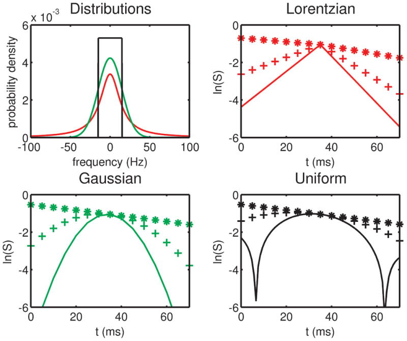
The three frequency distributions considered here—Lorentzian (red), Gaussian (green) and uniform (black)—are shown on the top left, each with a central frequency of 0 Hz and width parameter (R₂′, σ or Δw) of 15 Hz. Also shown are the simulated time-domain signal magnitudes (see Eqs. [7-10]) for the Lorentzian (top right), Gaussian (bottom left) and uniform (bottom right) distributions, using width parameters of 5 Hz (*), 60 Hz (+) and 110 Hz (-), an irreversible relaxation rate R₂ of 15 Hz and a value of τ = 35 ms. Recall that t = 0 in Eqs. [7-10] corresponds to the time of the refocusing pulse, and therefore the spin-echo occurs at t = τ = 35 ms, which is equivalent to a spin-echo time (measured from the time of the excitation pulse) of 70 ms.

Fig. 2 presents results from the 1.5T potato study demonstrating, in the case of strong reversible relaxation compared to irreversible relaxation, the possibility of both Lorentzian and Gaussian model behavior. Shown at the top of the figure are five of the individual gradient-echo images, with the spin-echo occurring at a TE of 55 ms. All of the ln(S) versus time curves (lower plots) showed growth and then decay through the spin-echo as sampled from the individual gradient-echoes, indicating larger reversible relaxation than irreversible relaxation (2), presumably due to air pockets in the potato. In most of the potato flesh voxels, the ln(S) time courses displayed curvature and a leftward shift of the peak signal, consistent with Gaussian rather than Lorentzian intra-voxel frequency distributions. There were some locations, however, near the diseased portion of the potato (presumably fungi—a common potato blight) where straight lines, characteristic of Lorentzian distributions, were observed (Fig. 2, lower middle plot).

Fig. 2.

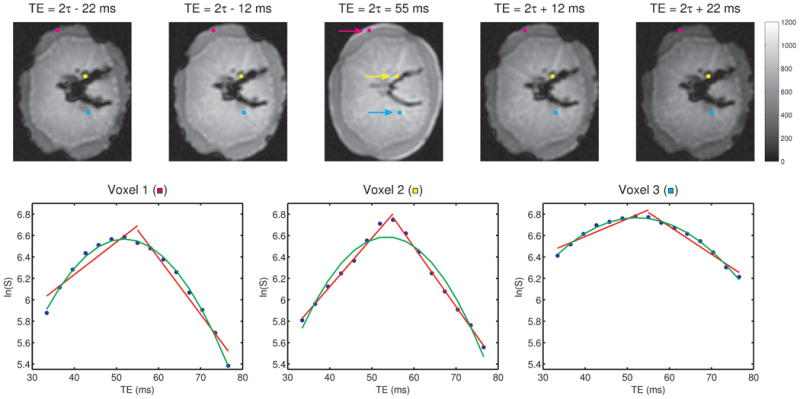
For the potato scanned at 1.5T, images corresponding to five of the echoes from the GESSE sequence are shown in the upper row, illustrating the left and right gradient-echo sampling of the spin-echo, with the central gradient-echo coinciding with the spin-echo (TE = 55 ms). Semi-log plots of signal magnitude versus echo time are shown in blue in the lower row, along with Lorentzian (red) and Gaussian (green) fits, for the voxels marked with purple, yellow and cyan squares in the upper row. These three voxels are located in the outer layer of the potato (lower left plot), the diseased area (lower middle plot) and the central region (lower right plot), respectively. Note that only in the diseased portion of the potato does the Lorentzian fit outperform the Gaussian fits found within the healthy regions of the potato.

Fig. 3 presents results from the 1.5T brain study. A semi-log plot of signal intensity versus echo time is shown (top left) for the voxel marked with the purple square in the other images, demonstrating a far better fit to the Gaussian model than the Lorentzian. Specifically, significant departures from straight lines on either side of the inflection point at the spin-echo position, which would be characteristic of Lorentzian distributions on such plots, were observed along with a leftward shift of the echo signal maximum, all characteristic of Gaussian distributions as predicted from the model simulations shown in the bottom left of Fig. 1. A map of the simple “quality of fit” measure described in the Methods section is shown on the bottom left of Fig. 3, showing that the two models perform equally well in most of the brain, but that the Gaussian model clearly wins in many regions (such as the one surrounding the purple square). Also shown in Fig. 3 are the irreversible relaxation rate (R₂) maps from the Lorentzian and Gaussian fits (middle panel), in which subtle but real differences can be observed (vide infra), and the corresponding width maps (right panel), in which more structure is apparent in the Gaussian σ map than the Lorentzian R₂′ map. From inspection of this figure and as confirmed by examining time-domain spin-echo signals from multiple brain voxels, we observed that in voxels where the irreversible relaxation dominates, the two models perform equally well, but in voxels where the reversible relaxation is comparable to or greater than the irreversible relaxation, the Gaussian model typically provides a better fit. In short, for voxels within the brain, the Lorentzian model hardly ever outperformed the Gaussian model.

Fig. 3.

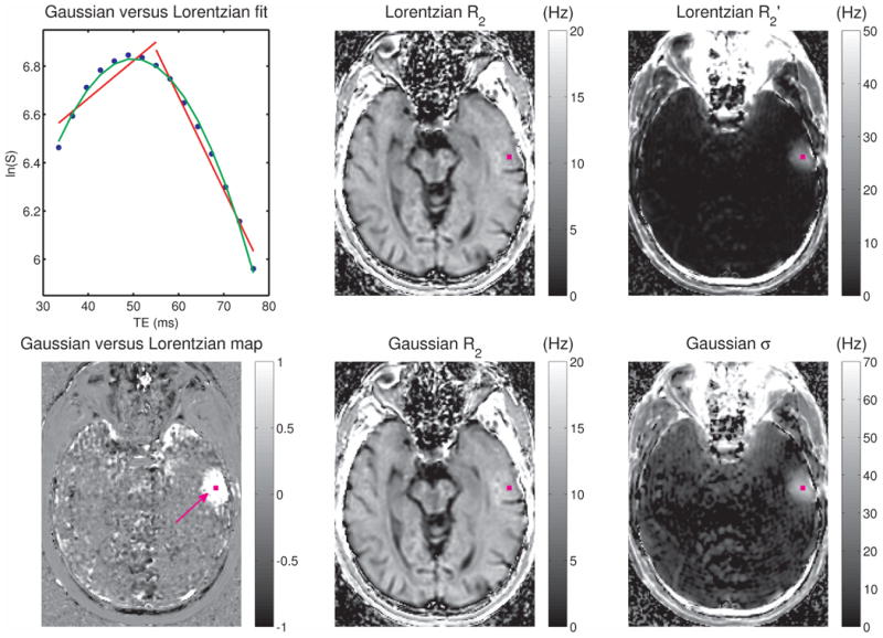
For the 15 echoes collected at 1.5T on the human subject using the GESSE sequence (with τ = 27.5 ms, corresponding to a spin-echo time of 55 ms), a semi-log plot of signal magnitude versus echo time is shown in blue on the top left for the voxel marked with a purple square in the remaining images. Fits assuming either a Lorentzian or a Gaussian distribution are shown in red and green, respectively. Note that a distinct departure from the echo-time dependence of a Lorentzian frequency distribution is observed for this voxel, whereas the Gaussian distribution model provides an excellent fit to the data. For each voxel, the simple “quality of fit” measure described in the Methods section was computed, and this map is shown on the bottom left. Intensities near zero (medium gray) in this image indicate regions where the two models performed equally well, whereas intensities greater than zero (white) indicate regions where the Gaussian model outperformed the Lorentzian. Also shown are the irreversible relaxation rate (R₂) maps as obtained from the Lorentzian (top center) and Gaussian (bottom center) fits, along with the corresponding width maps R₂′ (top right) and σ (bottom right). All relaxation rates and frequency widths are in Hz.

Fig. 4 presents results from a 3T scan of the same subject shown in Fig. 3. Again, note the significant curvature of the ln(S) time course for the highlighted voxel, resulting in a superior fit for the Gaussian model. Gaussian and Lorentzian fits were of comparable quality in this slice in the occipital lobe towards the back of the head, as well as in central regions in higher slices where the irreversible relaxation was dominant. However, Gaussian fits significantly outperformed Lorentzian fits in many voxels, especially those in frontal regions near sinuses (see Fig. 4, bottom left), where the reversible relaxation was significant. Comparing the width maps at the two field strengths (right panel of Figs. 3 and 4), we see greater values at 3T regardless of model distribution, as would be expected due to greater susceptibility effects, leading to more structure being apparent in the width maps at the higher field strength. Note also that here the 3T data is noisier than the 1.5T data, since the gain in SNR due to field strength is more than offset by a combination of longer echo times, shorter TR, smaller voxel size and higher readout bandwidth.

Fig. 4.

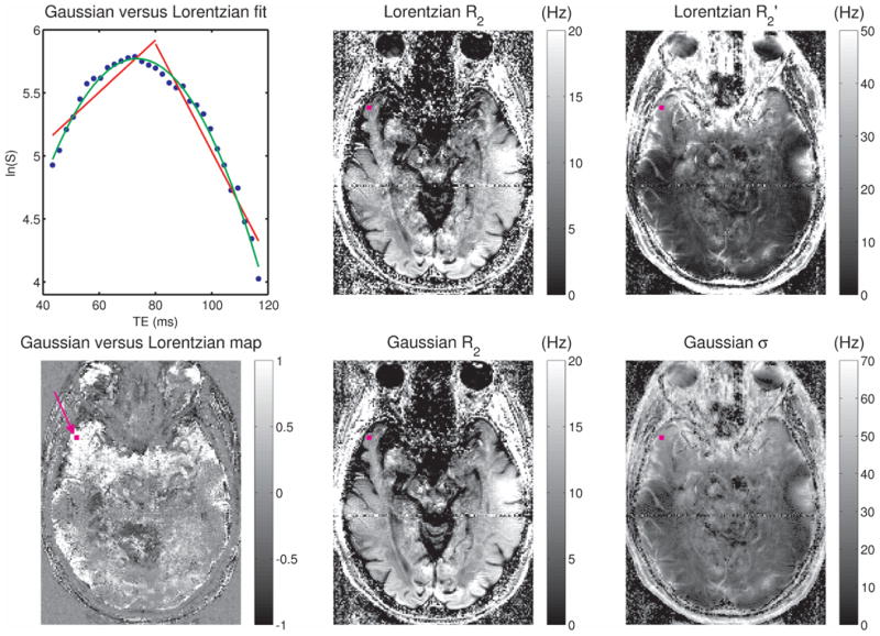
For the same subject shown in Fig. 3, results are shown here for data collected at 3T, using an implementation of the GESSE sequence with 31 echoes and spin-echo at 80 ms (τ = 40 ms). As in Fig. 3, a semi-log plot of signal magnitude versus echo time is shown in blue on the top left for the voxel marked with a purple square in the remaining images, overlaid with Lorentzian (red) and Gaussian (green) fits. The quality of fit map is shown on the bottom left, the R₂ maps obtained via the Lorentzian and Gaussian fits are shown in the middle panel, and the width maps (Lorentzian R₂′ and Gaussian σ) are shown in the right panel. All relaxation rates and frequency widths are in Hz.

To see how the choice of model affects the estimation of irreversible relaxation rates, the R₂ values obtained via the Gaussian fit were compared to the corresponding values obtained from a Lorentzian fit (see Fig. 5, middle panel). Although the correlation between the two R₂ values was good overall (r² = 0.84), substantial differences were observed for some voxels. A slight bias towards higher R₂ values is also seen for estimates obtained via the Lorentzian versus the Gaussian model. In the right panel of Fig. 5, R₂ values from the Gaussian fit are compared to the model-free R₂ values estimated using the procedure described in the Methods, showing a remarkable agreement between these two estimates (r² > 0.99).

Fig. 5.

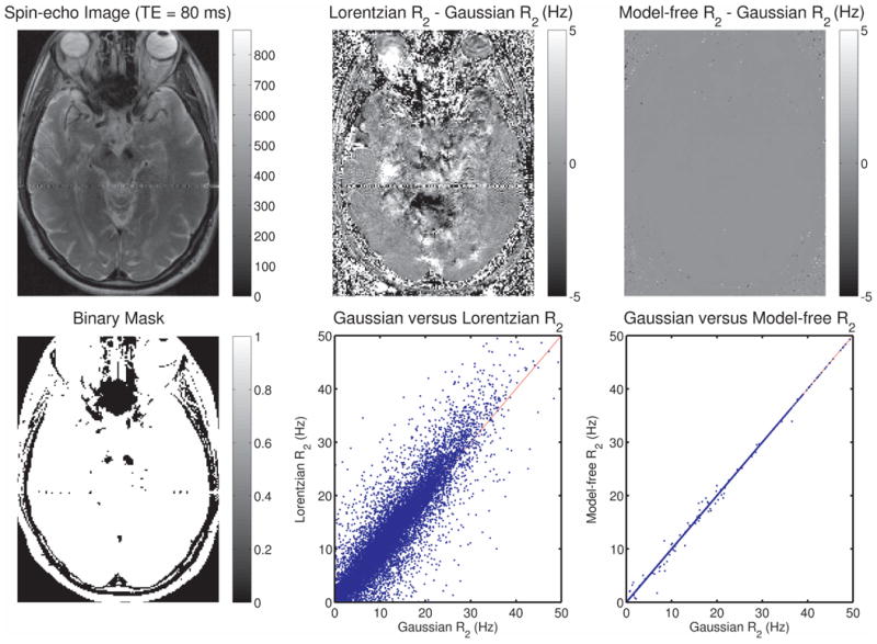
The spin-echo image for the same slice as in Fig. 4 is shown on the top left (3T data). A subtraction image of the R₂ maps obtained via Gaussian versus Lorentzian fits is shown on the top center, and a subtraction image of the R₂ maps obtained via Gaussian fitting versus the model-free R₂ estimation procedure described in the text is shown on the top right. Voxels with intensity greater than 100 were selected from the spin-echo image and the corresponding binary mask is shown on the bottom left. For these voxels, the R₂ values obtained via the Gaussian fit are plotted against the corresponding values obtained from the Lorentzian fit (bottom center), showing differences on the order of 5-10%, with the squared correlation coefficient r² = 0.84. On the bottom right, the Gaussian R₂ values are plotted against the values from the model-free R₂ estimates (r² > 0.99).

Since R₂* mapping is of relevance to iron deposition studies and has more recently sparked interest for use with ultra-high field (7T) brain imaging (23), it is of interest to consider what the equivalent map would be when a Gaussian model as opposed to a Lorentzian model is employed. Fig. 6 shows the familiar R₂* map calculated assuming a Lorentzian model (with R₂* = R₂ + R₂′) as well as a “σ*” map calculated assuming a Gaussian model (with σ* = R₂ + σ). In both cases the relevant width parameter of the frequency distribution has been added to the irreversible relaxation rate R₂. The two images in Fig. 6 are windowed identically and share similar features though with somewhat larger values for the reversible + irreversible transverse relaxation parameters obtained for the σ* maps.

Fig. 6.

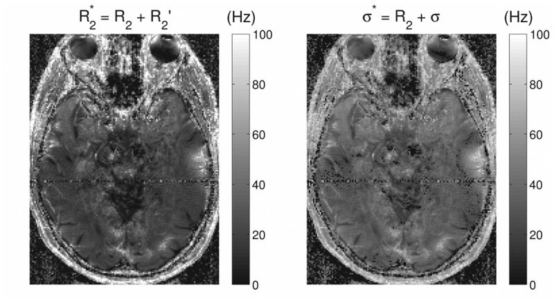
The R₂ and frequency width maps shown in Fig. 4 were combined to produce an R₂* map (left), which assumes a Lorentzian model (with R₂* = R₂ + R₂′), and a “σ*” map (right), which assumes a Gaussian model (with σ* = R₂ + σ). Both R₂* and σ* have units of Hz.

Finally, we examine data from the putamen and pallidum, iron-containing structures studied in the past with GESFIDE/GESSE sequences or variants thereof. Fig. 7 shows 1.5T and 3T spin-echo images and plots of ln(S) versus time from single voxels in these two structures and several points of interest may be made here. Namely, at 1.5T, irreversible relaxation is much larger than reversible relaxation in these structures, leading to a decay of signal throughout the entire echo and making the choice between Lorentzian (red) and Gaussian (green) models largely irrelevant. At 3T, however, reversible relaxation has become as large or larger in these structures, resulting in a small growth of signal on the left side of the echo and some curvature in the ln(S) time courses. These signals thus appear to be better suited to Gaussian than Lorentzian models even given the modest SNR in these voxels.

Fig. 7.

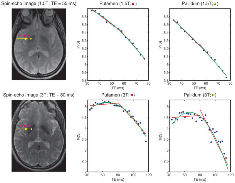
Spin-echo images at 1.5T (top left) and 3T (bottom left), with single voxels in the putamen and pallidum marked with purple and yellow squares, respectively. The middle panel shows, for each field strength, plots of ln(S) versus time for the putamen voxels marked on the spin-echo images and the right panel shows the corresponding plots for the pallidum voxels. Note that at 1.5 T, irreversible relaxation is much larger than reversible relaxation in these iron-containing structures, leading to decay of signal throughout the entire echo and making the choice between Lorentzian (red) and Gaussian (green) models largely irrelevant. At 3T, however, reversible relaxation has become as large or larger in these structures, resulting in a small growth of signal on the left side of the spin echo and in some curvature in the ln(S) time courses, which therefore appear more suited to modeling with Gaussian distributions.

Discussion and Conclusions

In many regions of the brain distal from air/tissue or air/bone interfaces where irreversible relaxation rates were generally larger than reversible relaxation rates, Gaussian and Lorentzian fits to the data were of similar quality. In frontal regions of grey matter situated near sinuses, however, significant curvature of ln(S) time courses was observed, with a left-shifted echo peak, characteristic of Gaussian frequency distributions. Indeed, in these cases, Gaussian fits significantly outperformed Lorentzian fits in terms of overall ability to adequately characterize the shapes of the signal time courses. In these regions, differences of ∼10% in the irreversible relaxation rates R₂ arose between the two types of fit. Presumably, with more accurate evaluation of the reversible relaxation process attained with the Gaussian fits, more accurate representation of the irreversible relaxation is also attained since both are estimated simultaneously from fits to the experimental data.

Within the context of quantitative transverse relaxation imaging, a number of methods are available, all with varying degrees of complexity, information content and potential for artifact. For example, Carr-Purcell-Meiboom-Gill (CPMG) imaging sequences with non-selective refocusing pulses and appropriate spoiling schemes, as discussed by Poon and Henkelman (24), may be applied in single-slice mode or 3D mode to assess irreversible relaxation in great detail. Mackay and colleagues have long espoused this approach for studying the multicompartmental nature of brain water as accessed with multiexponential fits of CPMG decay curves to separate, for example, myelin-associated water with a very short T₂ (approximately 5 to 30 ms) from water within and between brain cells with longer T₂ values (25). Difficulties with the CPMG approach include long scan times and the artifactual effects of stimulated echoes from imperfect refocusing pulses, particularly at high field, ultimately involving complicated schemes for correction (21). In addition, one does not get a measure of the reversible relaxation rate from CPMG approaches. Furthermore, the irreversible relaxation rate, estimated from multiple spin-echoes with short inter-echo spacings, can be anticipated to differ from that measured with a GESFIDE/GESSE approach that utilizes a single Hahn spin-echo. Namely, contributions from diffusion within the gradients and/or background frequency distributions as well as water exchange between compartments will be different between these two methods such that, in general, smaller irreversible relaxation rates can be anticipated with CPMG versus GESFIDE/GESSE methods.

A remarkable aspect of the GESFIDE/GESSE approaches is that, with nuisance terms removed via spoiling and/or phase cycling (vide supra), it is difficult to conceive of artifactual influences to the data, particularly for GESSE in which the potentially different slice profile issues which may affect GESFIDE are avoided (5). The beauty of GESFIDE and GESSE approaches thus lies in (i) their relatively brief scan times for multi-slice full brain volume coverage, (ii) their relative insensitivity to B_o and B₁ artifacts and (iii) the simultaneous estimation of both reversible and irreversible relaxation rates. Although we have not explicitly considered pure gradient-echo FID sampling in this work, the data we have collected on the right side of the spin-echo has implications for such sampling. Namely, in regions where we have observed signal time courses strongly indicative of Gaussian frequency distributions, multiple gradient-echo sampling following a single excitation is expected to show similar curvature. A complete comparison of how the second half of spin-echoes collected at 50 ms or longer compared to FID sampling, in which presumably myelin-associated water also contributes (26), is beyond the scope of this work but is certainly worthy of further attention within the context of quantitative transverse relaxation studies of the brain.

Finally, we note that we have to date only focused upon magnitude image data but that the time course of the phase data through a spin-echo as sampled with gradient-echoes could also be of value in spatially mapping the central frequencies (w_o) of the distributions and possibly correcting for strong background gradients (27). In this context, GESFIDE/GESSE sequences might be employed in a manner similar to that which has been demonstrated with asymmetric spin-echo sequences, an early version of which was used to demonstrate spin-echo time courses indicative of Gaussian distributions in excised rat lungs (28), with more recent versions adapted for iron deposition studies (29,30).

In conclusion, our studies show that modeling the time course of spin-echoes in some regions of the brain with GESFIDE/GESSE type sequences may be better performed with Gaussian rather than Lorentzian models of the underlying frequency distributions responsible for reversible relaxation. We further propose that, in this manner, more accurate (or, at least, less artifact-prone) values for the irreversible relaxation rates R₂ may be obtained, particularly at higher fields such as 3T and above where reversible relaxation effects become more prominent.

Appendix

Bloch Equation Tools

We have used only three mathematical tools to perform the Bloch equation single isochromat analyses in each of the pulse sequence segments discussed above. These are two rotation matrices representing the effects of RF pulses along the x- and y-axes of the rotating frame. For the time in between these pulses, a free precession/relaxation matrix with the addition of a vector component to account for longitudinal spin-lattice relaxation was employed.

The following two rotation matrices are used to represent the effects of RF pulses with flip angle θ along the x- and y-axis of the rotating frame, respectively:

$$\begin{array}{ccccc}& & 1& 0& 0\\ {\mathrm{\theta }}_{\mathrm{x}}& =& 0& cos\mathrm{\theta }& sin\mathrm{\theta }\\ & & 0& -sin\mathrm{\theta }& cos\mathrm{\theta }\end{array}$$ [A1]

$$\begin{array}{ccccc}& & cos\mathrm{\theta }& 0& sin\mathrm{\theta }\\ {\mathrm{\theta }}_{\mathrm{y}}& =& 0& 1& 0\\ & & -sin\mathrm{\theta }& 0& cos\mathrm{\theta }\end{array}$$ [A2]

Apologies to purists who like their rotations to have a strictly « positive » bent as in the latter case the matrix represents a negative rotation about the y-axis.

The free precession/relaxation (PR) plus longitudinal relaxation between pulses, for time t, is taken care of using

$$\text{PR}=\begin{array}{ccc}cos(\mathrm{w}\mathrm{t})exp(-{\mathrm{R}}_2\mathrm{t})& sin(\mathrm{w}\mathrm{t})exp(-{\mathrm{R}}_2\mathrm{t})& 0\\ -sin(\mathrm{w}\mathrm{t})exp(-{\mathrm{R}}_2\mathrm{t})& cos(\mathrm{w}\mathrm{t})exp(-{\mathrm{R}}_2\mathrm{t})& 0\\ 0& 0& exp(-{\mathrm{R}}_1\mathrm{t})\end{array}+\begin{array}{c}0\\ 0\\ {\mathrm{m}}_{\text{oo}}(1-exp(-{\mathrm{R}}_1\mathrm{t}))\end{array}$$ [A3]

Spoiling Considerations

Spoiling/crushing in a spin-echo sequence in which the flip angle β of the refocusing pulse deviates from a perfect 180° is commonly performed and consists of sandwiching the refocusing pulse between a pair of unipolar field gradient pulses. We consider this phenomenon by analyzing a 90_y – τ₁ – τ_s – β_x - τ_s – t sequence in which a gradient pulse of amplitude G is applied along the z direction during the τ_s periods. Assuming that the steady-state magnetization prior to the 90_y excitation pulse is all longitudinal and given by m_o, with the equilibrium longitudinal magnetization being m_oo, a Bloch equation analysis yields the signal S = f + ig as a function of time t during the readout as

$$\begin{array}{lll}\mathrm{S}\hfill & =\hfill & ({\mathrm{m}}_{\mathrm{o}}/2)(1-cos\mathrm{\beta })exp(-{\mathrm{R}}_2({\mathrm{\tau }}_1+2{\mathrm{\tau }}_{\mathrm{S}}+\mathrm{t}))exp({\text{iw}}_{\mathrm{o}}({\mathrm{\tau }}_1-\mathrm{t}))\hfill \\ \hfill & \hfill & +({\mathrm{m}}_{\mathrm{o}}/2)(1+cos\mathrm{\beta })exp(-{\mathrm{R}}_2({\mathrm{\tau }}_1+2{\mathrm{\tau }}_{\mathrm{S}}+\mathrm{t}))exp(-{\text{iw}}_{\mathrm{o}}({\mathrm{\tau }}_1+2{\mathrm{\tau }}_{\mathrm{S}}+\mathrm{t}))exp(-{\text{iw}}_{\mathrm{z}}2{\mathrm{\tau }}_{\mathrm{S}})\hfill \\ \hfill & \hfill & +{\text{im}}_{\text{oo}}sin\mathrm{\beta }exp(-{\mathrm{R}}_2({\mathrm{\tau }}_{\mathrm{S}}+\mathrm{t}))[1-exp(-{\mathrm{R}}_1({\mathrm{\tau }}_1+{\mathrm{\tau }}_{\mathrm{S}}))]exp(-{\text{iw}}_{\mathrm{o}}({\mathrm{\tau }}_{\mathrm{S}}+\mathrm{t}))exp({\text{iw}}_{\mathrm{z}}{\mathrm{\tau }}_{\mathrm{S}})\hfill \end{array}$$ [A4]

where R₁ and R₂ are the longitudinal and irreversible transverse relaxation rates, respectively, w_o is the frequency offset in the absence of the spoiling gradient and w_z the position dependent frequency during the spoiling periods t_s. Eq. [A4] demonstrates that the signal is comprised of three primary terms each with a different dependence on the refocusing flip angle β: (i) 1 - cosβ, (ii) 1 + cosβ and (iii) sinβ. The latter two vanish for β = 180°. However, in the unavoidable absence of this condition, the spoiling gradients are relied upon to minimize the contributions from these last two “nuisance” terms. Note that the “money” term proportional to (1 – cosβ) has no w_z dependence which is why it is unaffected by the spoiler gradients. To see the effect of w_z on each of the other terms we must consider integrating exp(-iw_z2τ_s) and exp(-iw_zτ_s), respectively, over relevant ranges of w_z. Let us consider spoiling along the slice selection direction and calculate spoiling factors SP(G,τ_s,Δz) for each of the nuisance terms where Δz is the slice thickness representative of the distance over which the spoiling occurs. For the (1 + cosβ) term we have

$$\begin{array}{lll}\text{SP}(\mathrm{G},{\mathrm{\tau }}_{\mathrm{S}},\mathrm{\Delta }\mathrm{z})\hfill & =\hfill & (1/\mathrm{\Delta }\mathrm{z})\underset{{\mathrm{z}}_{\mathrm{o}}-\mathrm{\Delta }\mathrm{z}/2}{\overset{{\mathrm{z}}_{\mathrm{o}}+\mathrm{\Delta }\mathrm{z}/2}{\int }}exp({\text{iw}}_{\mathrm{z}}2{\mathrm{\tau }}_{\mathrm{S}})\text{dz}\hfill \\ \hfill & =\hfill & (1/\mathrm{\Delta }\mathrm{z})\underset{{\mathrm{z}}_{\mathrm{o}}-\mathrm{\Delta }\mathrm{z}/2}{\overset{{\mathrm{z}}_{\mathrm{o}}+\mathrm{\Delta }\mathrm{z}/2}{\int }}exp(-i({\mathrm{w}}_{\mathrm{o}}+\gamma \text{Gz}))(2{\mathrm{\tau }}_{\mathrm{S}})\text{dz}\hfill \end{array}$$ [A5]

where the limits of the integration reflect the slice thickness and the central location z_o of the slice. Note the normalization of this integral by the slice thickness to insure a unitless spoiling factor. Performing the requisite integration we obtain

$$\text{SP}(\mathrm{G},{\mathrm{\tau }}_{\mathrm{S}},\mathrm{\Delta }\mathrm{z})=exp(-{\text{iw}}_{\mathrm{o}}2{\mathrm{\tau }}_{\mathrm{S}})exp(-i\gamma {\text{Gz}}_{\mathrm{o}}2{\mathrm{\tau }}_{\mathrm{S}})sin(\gamma \mathrm{G}\mathrm{\Delta }\mathrm{z}{\mathrm{\tau }}_{\mathrm{S}})/(\gamma \mathrm{G}{\mathrm{\tau }}_{\mathrm{S}}\mathrm{\Delta }\mathrm{z}).$$ [A6]

The spoiling factor for the sinβ term is similar but with τ_s replaced by τ_s/2 in Eq. [A6] as this term arises from magnetization aligned along the longitudinal axis in between the two RF pulses and so does not experience any dephasing during the first τ_s period. Clearly, the larger the gradient G and τ_s, the greater degree of spoiling but note that choosing the argument of the sinc function in Eq. [A6] wisely can also lead to increased spoiling efficiency, e.g., by choosing a zero of the sinc. It is interesting to consider asymmetric spoiler gradients such as a plus/minus combination about the refocusing in which case the (1 + cosβ) term is unaffected and the (1 - cosβ) term is spoiled (proof left to the reader).

References

- 1.Hahn EL. Spin echoes. Phys Rev. 1950;80:589–594. [Google Scholar]
- 2.Ma J, Wehrli FW. Method for image-based measurement of the reversible and irreversible contribution to the transverse-relaxation rate. J Magn Reson B. 1996;111:61–69. doi: 10.1006/jmrb.1996.0060. [DOI] [PubMed] [Google Scholar]
- 3.Ordidge RJ, Gorell JM, Deniau JC, Knight RA, Helpern JA. Assessment of relative brain iron concentrations using T2-weighted and T2* weighted MRI at 3 Tesla. Magn Reson Med. 1994;32:335–341. doi: 10.1002/mrm.1910320309. [DOI] [PubMed] [Google Scholar]
- 4.Yang X, Cao J, Wang X, Li X, Xu Y, Jiang X. Evaluation of renal oxygen in rat by using R2′ at 3T magnetic resonance: initial observation. Acad Radiol. 2008;15:912–918. doi: 10.1016/j.acra.2008.01.015. [DOI] [PubMed] [Google Scholar]
- 5.Yablonskiy DA, Haacke EM. An MRI method for measuring T2 in the presence of static and RF magnetic field inhomogeneities. Magn Reson Med. 1997:872–876. doi: 10.1002/mrm.1910370611. [DOI] [PubMed] [Google Scholar]
- 6.Gelman N, Gorell JM, Barker PB, Savage RM, Spickler EM, Windham JP, Knight RA. MR imaging of human brain at 3.0 T: Preliminary report on transverse relaxation rates and relation to estimated iron content. Radiology. 1999;210:759–767. doi: 10.1148/radiology.210.3.r99fe41759. [DOI] [PubMed] [Google Scholar]
- 7.Hikita T, Abe K, Sakoda S, Tanaka H, Murase K, Fujita N. Determination of transverse relaxation rate for estimating iron deposits in central nervous system. Neuroscience Research. 2005;51:67–71. doi: 10.1016/j.neures.2004.09.006. [DOI] [PubMed] [Google Scholar]
- 8.Allen RP, Barker PB, Wehrli F, Song HK, Earley CJ. MRI measurement of brain iron in patients with restless leg syndrome. Neurology. 2001;56:263–265. doi: 10.1212/wnl.56.2.263. [DOI] [PubMed] [Google Scholar]
- 9.Welch KMA, Nagesh V, Aurora SK, Gelman N. Periaqueductal gray matter dysfunction in migraine: Cause or the burden of illness? Headache. 2001;41:629–637. doi: 10.1046/j.1526-4610.2001.041007629.x. [DOI] [PubMed] [Google Scholar]
- 10.Hendry J, DeVito T, Gelman N, Densmore M, Rajakumar N, Pavlosky W, Williamson PC, Thompson PM, Drost DJ, Nicolson R. White matter abnormalities in autism detected through transverse relaxation time imaging. NeuroImage. 2006;29:1049–1057. doi: 10.1016/j.neuroimage.2005.08.039. [DOI] [PubMed] [Google Scholar]
- 11.Khalil M, Langkammer C, Ropele S, Petrovic K, Wallner-Blazek M, Loitfelder M, Jehna M, Bachmaier G, Schmidt R, Enzinger C, Fuchs S, Fazekas F. Determinants of brain iron in multiple sclerosis: A quantitative 3T MRI study. Neurology. 2011;77:1691–1697. doi: 10.1212/WNL.0b013e318236ef0e. [DOI] [PubMed] [Google Scholar]
- 12.Miszkiel KA, Paley MNJ, Wilkinson ID, Hall-Craggs MA, Ordidge R, Kendall BE, Miller RF, Harrison MJG. The measurement of R2, R2* and R2′ in HIV-infected patients using the PRIME sequence as a measure of brain iron deposition. Magn Reson Imag. 1997;15:1113–1119. doi: 10.1016/s0730-725x(97)00089-1. [DOI] [PubMed] [Google Scholar]
- 13.Graham JM, Paley MNJ, Grunewald RA, Hoggard N, Grifiths PD. Brain iron deposition in Parkinson's disease imaged using the PRIME magnetic resonance sequence. Brain. 2000;123:2423–2431. doi: 10.1093/brain/123.12.2423. [DOI] [PubMed] [Google Scholar]
- 14.Song R, Cohen AR, Song HK. Improved transverse relaxation rate measurement techniques for the assessment of hepatic and myocardial content. J Magn Reson Imaging. 2007;26:208–214. doi: 10.1002/jmri.20994. [DOI] [PubMed] [Google Scholar]
- 15.Jin N, Guo Y, Zhang Z, Zhang L, Lu G, Larson AC. GESFISE-PROPELLER approach for simultaneous R2 and R2* measurements in the abdomen. Magn Reson Imag. 2013;31:1760–1765. doi: 10.1016/j.mri.2013.08.003. [DOI] [PMC free article] [PubMed] [Google Scholar]
- 16.Song R, Song HK. Echo-spacing optimization for the simultaneous measurement of reversible (R2′) and irreversible (R2) transverse relaxation rates. Magn Reson Imag. 2007;25:63–68. doi: 10.1016/j.mri.2006.09.008. [DOI] [PMC free article] [PubMed] [Google Scholar]
- 17.Mulkern RV, Balasubramanian M, Orbach DB, Mitsouras D, Haker SJ. Incorporating reversible and irreversible transverse relaxation effects into steady state free precession (SSFP) signal intensity expressions for fMRI considerations. Magn Reson Imag. 2013;31:346–352. doi: 10.1016/j.mri.2012.10.002. [DOI] [PubMed] [Google Scholar]
- 18.Azzalini A. A class of distributions which includes the normal ones. Scand J Statist. 1985;12:171–178. [Google Scholar]
- 19.Marsden JE. Basic Complex Analysis. Freeman; San Francisco, CA: 1973. [Google Scholar]
- 20.Gradshteyn IS, Ryzhik IM. Table of Integrals, Series, and Products. Seventh. Academic Press; Burlington, MA: [Google Scholar]
- 21.Prasloski T, Burkhard M, Xiang QS, MacKay A, Jones C. Applications of stimulated echo correction to multicomponent T2 analysis. Magn Reson Med. 2012;67:1803–1814. doi: 10.1002/mrm.23157. [DOI] [PubMed] [Google Scholar]
- 22.Meiboom S, Gill D. Modified spin-echo method for measuring nuclear relaxation times. Rev Sci Instrum. 1958;29:668–691. [Google Scholar]
- 23.Deistung A, Schafer A, Schweser F, Biedermann U, Gullmar D, Trampel R, Turner R, Reichenbach JR. High resolution MR imaging of the human brainstem in vivo at 7 Tesla. Frontiers in Human Neuroscience. 2013;7:1–12. doi: 10.3389/fnhum.2013.00710. article 710. [DOI] [PMC free article] [PubMed] [Google Scholar]
- 24.Poon C, Henkelman RM. T2 quantification for clinical applications. J Magn Reson Imag. 1992;2:541–553. doi: 10.1002/jmri.1880020512. [DOI] [PubMed] [Google Scholar]
- 25.MacKay AL, Whittall KP, Adler J, Li DKB, Paty DW, Graeb D. In vivo visualization of myelin water in brain by magnetic resonance. Magn Reson Med. 1994;31:673–677. doi: 10.1002/mrm.1910310614. [DOI] [PubMed] [Google Scholar]
- 26.Du YP, Chu R, Hwang D, Brown MS, Kleinschmidt-Demasters BK, Singel D, Simon JH. Fast multislice mapping of myelin water fraction using multicompartment analysis of T2* decay at 3T: A preliminary postmortem study. Magn Reson Med. 2007;58:865–870. doi: 10.1002/mrm.21409. [DOI] [PubMed] [Google Scholar]
- 27.Sedlacik J, Boelmans K, Lobel U, Holst B, Siemonsen S, Fiehler J. Reversible, irreversible and effective transverse relaxation rates in aging brain at 3 T. NeuroImage. 2013;84:1032–1041. doi: 10.1016/j.neuroimage.2013.08.051. [DOI] [PubMed] [Google Scholar]
- 28.Ganesan K, Ailion DC, Cutillo AG, Goodrich KC. New technique for obtaining NMR linewidth images of lung and other inhomogeneously broadened systems. J Magn Reson B. 1993;102:293–298. [Google Scholar]
- 29.Jensen JH, Chandra R, Ramani A, Lu H, Johnson G, Lee SP, Kaczynski K, Helpern JA. Magnetic field correlation imaging. Magn Reson Med. 2006;55:1350–1361. doi: 10.1002/mrm.20907. [DOI] [PubMed] [Google Scholar]
- 30.Dumas EM, Versluis MJ, van den Bogaard SJA, van Osch MJP, Hart EP, van Roon-Mom WMC, van Buchem MA, Webb AG, van der Grond J, Roos RAC. Elevated brain iron is independent from atrophy in Huntington's disease. NeuroImage. 2012;61:558–564. doi: 10.1016/j.neuroimage.2012.03.056. [DOI] [PubMed] [Google Scholar]