Contending with uncertainty in conservation management decisions

Abstract

Efficient conservation management is particularly important because current spending is estimated to be insufficient to conserve the world's biodiversity. However, efficient management is confounded by uncertainty that pervades conservation management decisions. Uncertainties exist in objectives, dynamics of systems, the set of management options available, the influence of these management options, and the constraints on these options. Probabilistic and nonprobabilistic quantitative methods can help contend with these uncertainties. The vast majority of these account for known epistemic uncertainties, with methods optimizing the expected performance or finding solutions that achieve minimum performance requirements. Ignorance and indeterminacy continue to confound environmental management problems. While quantitative methods to account for uncertainty must aid decisions if the underlying models are sufficient approximations of reality, whether such models are sufficiently accurate has not yet been examined.

Introduction

Faced with large contemporary extinction of species, degradation of ecosystems, fragmentation of remaining indigenous vegetation, and uncertain fates for many species, resources that are available to conserve biodiversity must be spent efficiently. Efficient management is particularly important because current spending is estimated to be insufficient to conserve the world's biodiversity; indeed, a 10-fold increase in funding might be necessary.¹

The logic of decision making in conservation management to achieve efficient outcomes is conceptually straight-forward. Effective conservation management relies on managers specifying:^2,3

• (1) Goals—what they want to achieve, and how these objectives will be measured;

• (2) Threats and opportunities—the factors that influence objectives, including those that the manager can control; and

• (3) Alternatives—the set of management actions available, how they influence the objectives, and any constraints on those actions.

Finally, from the set of management alternatives, managers should find those that best achieve the goals. While conceptually simple when described as these series of steps, uncertainty pervades many aspects of this approach, which can cloud efficient management.

This review examines these uncertainties, and highlights ways of characterizing and contending with uncertainty in conservation decisions. I discuss a range of probabilistic and nonprobabilistic methods, and the difficulty of accounting for ignorance in management decisions.

Conservation decisions are required for many different circumstances, such as decisions about whether species should be listed as threatened, choosing from a set of management strategies for those species, allocating land or seascapes to conservation management regimes of various forms or permitting development, determining search effort for invasive or threatened species, or deciding what monitoring should be conducted. I will illustrate and compare the range of approaches to dealing with uncertainty by drawing on a single example where a manager must decide on the search effort for an invasive species at a site. To maintain consistency, this will be a common (but relatively tractable) example throughout the review. In this case, the question is simply to determine how much effort should be expended in searching for a species at a site that might further harm biodiversity if it remains undetected. The same basic methods and ideas can be extended to other conservation decisions.

Before discussing where uncertainties arise in conservation decisions and illustrating a range of methods for contending with these uncertainties, I will summarize the taxonomy of uncertainty offered by Regan et al.⁴ Other classifications of uncertainty exist. For example, a recent review⁵ of classifications of uncertainty in environmental risk assessment recognizes different natures of uncertainty (whether the uncertainty is epistemic or a function of imprecise knowledge), the location (whether the uncertainty lies in, for example, the system, the data, the model, or human flaws), and the level of uncertainty (ranging from deterministic understanding to blind ignorance). This treatment and others are valuable, although here I use the taxonomy of Regan et al.

Taxonomy of uncertainty

Regan et al.⁴ identify two major forms of uncertainty relevant to conservation management. Epistemic uncertainty relates to uncertainty in facts of matters, and is the most commonly considered form of uncertainty in conservation.^6–8 It includes uncertainty in estimates or relationships among species (including imprecision and bias), natural variation such as in population dynamics arising from environments and their often unpredictable effects (e.g., effects of weather on population dynamics), and model uncertainty (e.g., uncertainty in the most appropriate way of describing relationships).

Regan et al.⁴ also noted that linguistic uncertainty is common in conservation problems, although less commonly acknowledged. Linguistic uncertainty arises because language is imprecise. Words can be ambiguous; for example, the term endangered has multiple different meanings. Even if a particular definition is used, such definitions rarely if ever, cater to borderline cases, leading to poor treatment of vagueness. Would we be prepared to accept that a species with 249 mature individuals is clearly endangered (according to the IUCN⁹), while a species with 250 mature individuals is not? Mature is another example of a word with ambiguity, and any definition based on age or reproductive ability might obscure vagueness that is inherent in defining maturity. Terms can also depend on context. The small population paradigm¹⁰ defines how small populations are more prone to extinction due to natural variation, yet the term small, as well as being vague, depends on context. A small population of bacteria might have many more individuals than even a large population of elephants. Some terms can be underspecified. For example, managers might wish to increase the future population size of a species, yet precise specification would define a particular rate of increase over a particular period of time. Finally, Regan et al.⁴ note that while some forms of linguistic uncertainty might not be apparent now, they can arise in the future; this is termed indeterminacy. Taxonomy provides many examples; current use of a particular taxonomic term (e.g., a species name) cannot reasonably envision the range of taxonomic revisions that might occur in the future. Similar incertitude arises in conservation decisions.

Some aspects of linguistic uncertainty also relate to aspects of epistemic uncertainty. For example, while variance in the population growth rate of a species might be estimated from the currently available data, indeterminacy means that these data from the past might not reliably estimate the variance in the future. Consider, for example, estimates of vital rates in the face of changing climates. Further, most estimates are context dependent; an estimate for survival of a species from one site might not apply to a second site.

Below I use these different forms of uncertainty to discuss how they can be addressed in different stages of conservation decision making.

Specifying and measuring objectives

Effective management relies on clearly articulated objectives. These define what management is trying to achieve and how success will be measured. Often, objectives of management are ambiguous and vague.³ One objective, for example, might be to protect biodiversity. More specifically, an objective might be to reduce the rate of biodiversity loss, such as in the Convention on Biological Diversity.¹¹ However, objectives can remain underspecified—how is biodiversity loss measured (e.g., for genetic diversity, species, and ecosystems) and what degree of reduction is sought?

Objectives can be organized hierarchically. Fundamental objectives¹² are typically vague and underspecified in policy;¹³ despite this linguistic uncertainty, they are important because they often reflect the regulatory environment in which decisions occur. Fundamental objectives often conflict with each other, which challenges decision making. For example, environmental decisions about managing a finite resource, such as forest timber or fish stocks, cannot indefinitely increase both short-term extractive benefits and conservation. Even relatively clear aims to increase persistence of species will often require trade-offs between increasing local versus global persistence. Clarifying the fundamental objectives helps separate important objectives from irrelevant ones; it is merely the first step in decision making but critical because effective decisions must account for all relevant objectives. Decisions made without considering important objectives are likely to be suboptimal.

Once the fundamental objectives are defined, means objectives make them measurable.¹⁴ Means objectives must be fully specified and as free from linguistic uncertainty as possible. They are sought not for their own sake but to achieve the fundamental objectives.¹² Where objectives conflict, they can be either weighted depending on relative preferences of the decision maker or analyzed separately to reveal trade-offs between them.¹⁵

For example, consider a manager searching for an invasive plant species at a site with the aim of eradicating the species by removing individuals if they are found.¹⁶ Assume the probability that the species is present before searching is 0.1. As searching continues, the probability that the species is present and remains undetected declines with the search time. The manager will aim to reduce this probability as much as possible; this is one objective. However, the manager will also wish to minimize the time spent searching; it is impossible to decrease one without increasing the other (Fig. 1). Other objectives might also impinge on the decision about allocating survey effort, such as understanding factors that influence the distribution of the species. Regardless of the number of objectives, the management decision boils down to considering the trade-offs between them.

Figure 1.

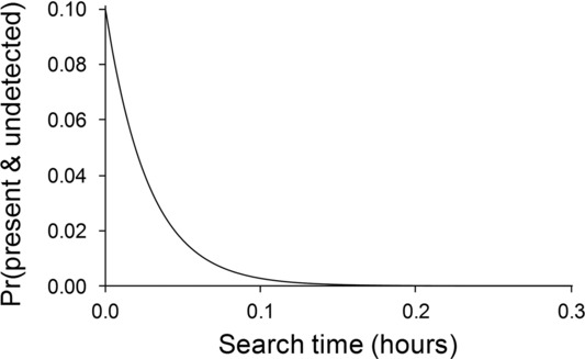
The trade-off between two quantities that a manager might wish to minimize when searching for an invasive species: the probability that the species is present and remains undetected, and the time spent searching.

Trade-offs between objectives are most easily assessed when they are measured in the same units. For example, the cost of a species being present but remaining undetected might be called the escape cost and expressed as the time required to manage the species in the future rather than now. When expressed in the same units such as this, we can simply trade one objective (survey costs) against the other (expected management costs), for example, by finding the search effort where the total expected cost (time spent surveying and managing) is minimized. However, if escape of the species at the site also entails costs that are difficult to measure in common units (e.g., the local extinction of a threatened species), trade-offs might become more uncertain. Further, escape costs might be unknown, depending on when the undetected species is eventually detected in the future. In this case, the manager needs to trade certain costs (the search time) against uncertain costs that might (or might not) be incurred at an uncertain time in the future. Such trade-offs are not necessarily trivial. I consider strategies for dealing with such uncertainties below (see the section “Choosing good management options”).

Objectives change over time, as seen in environmental regulations for most, if not all, of the world's countries. While managers might set objectives that reflect current regulatory environments, they might also seek to maintain options for future management.¹⁷ Managing to maintain options might suggest an incentive to err on the side of conservation over development;¹⁸ but the exact trade-off is clouded by the indeterminate future objectives. Indeterminacy in objectives is particularly pronounced when managing dynamic systems that might change (and possibly degrade) even when conserved.

Factors that influence the outcomes

Factors that influence the outcome of conservation management include the current state of the system being managed and how those states change both in the presence and absence of management. The first components are often referred to as system states. The second are defined by the dynamics of the system. System states typically include factors relevant to the means objectives. Examples include the nutrient levels when managing eutrophication of lakes,¹⁹ tree density when managing revegetation,²⁰ and the abundance of a species at a site at a particular point in time.²¹ Abundance might be the actual number of individuals or simplified to only presence or absence.²²

The dynamics of the system define how the states vary (e.g., over space and time). These dynamics are typically described by models. The models can include secondary state variables that influence the primary state variables (e.g., rainfall, which can influence population growth rates of species²³), particular functions that define relationships among variables, and the parameters of those functions.

Management variables define the factors that managers can change to influence conservation outcomes. Examples include the amount of survey effort to spend in an area,²² the number of animals to release from a captive breeding program,²⁴ which areas to set aside for conservation or other land uses,²⁵ the resources invested in conserving different species,^26,27 and the population parameters to target for the most efficient conservation outcome.²⁸

Many environmental decisions are framed with the assumption that the state of the system will be known. For example, optimal harvest problems are sometimes framed by setting harvest levels that depend on the abundance of the harvested stock. However, state variables, management variables, and system dynamics are typically subject to various forms of uncertainty. The most obvious is that state variables and model parameters will be measured with error (with imprecision and possible bias).

Uncertainty in the state of the system can be represented by adding belief states²⁹ that describe the state of knowledge. Belief states for parameter estimates might be defined by a probability distribution with a particular mean and variance. For example, McCarthy and Possingham²⁰ used beta probability distributions to define estimates of the probability of revegetation success for two different management actions. In other cases, belief states might describe the probability that a species is present.^22,30

Returning to the example of invasive species eradication in Figure 1, the trade-off between search time and the probability of the species being present but remaining undetected would be clouded by uncertainty in the presence of the species before searching (Fig. 2). The search effort that appropriately balances the trade-off in the objectives will typically be sensitive to the uncertain probability.

Figure 2.

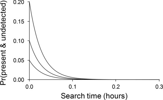
Three possible trade-offs between the probability that the species is present and remains undetected and the time spent searching. The trade-off depends on P, the probability that the species is present before the survey (P = 0.2, 0.1, 0.05).

In addition to parameter uncertainty, model uncertainty also exists. Managers will rarely know the best model to describe the dynamics of the system they are managing. Generally, a set of different models will be available, and each will fit the available data to different degrees. The fit of one model relative to others can be expressed in terms of weights that sum to one across all models in the set. These weights will typically reflect a trade-off between fit and parsimony.³¹ Decisions about the most appropriate action can depend on predictions that average over models. Alternatively, problems in which model weights can change over time, particularly as data accumulate, can be analyzed.³²

Managers can attempt to resolve uncertainty about the state of the system by targeted learning, which might then improve future decisions. However, this will usually come at the cost of immediate management actions. For example, the probability that a species is present at a site can be estimated by visiting multiple sites with high search effort (e.g., to eliminate false absences), which might then be used to optimize search effort at a new site (i.e., the estimate might help resolve the uncertainty depicted in Fig. 2). However, the effort spent on learning about the probability of presence could instead be allocated specifically to finding the species rather than to learning about its presence.

The optimal trade-off between learning and management is formally considered by using adaptive management. Adaptive management evaluates the benefits of obtaining information and the actions that result.^33–35 Passive adaptive management sets management objectives based on short-term goals, but collects information that will improve management in the future. Active adaptive management adjusts short term management to assist management with improved information, but only to the extent that long-term gains compensate for possible extra short-term costs.

Adaptive management recognizes that learning entails costs. Indeed, when deciding between two revegetation strategies with uncertain outcomes, McCarthy and Possingham²⁰ found that trialling both strategies simultaneously was rarely the best option even when monitoring was free. Using both options simultaneously entails a cost because inevitably an inferior strategy is used. When monitoring is not free, the two options are used even less frequently.³⁶ Delayed actions also entail costs, for example, due to ongoing degradation.³⁷

Adaptive management problems are typically solved with various forms of dynamic programming.³⁴ When accounting for uncertainty, the models usually suffer from the curse of dimensionality—in many cases, only relatively simple models have been solved. New algorithms for solving larger and more realistic problems are promising, and have been applied to conservation.³⁸ Nevertheless, computational skills are required that often mean managers must work collaboratively with computational scientists to find optimal solutions. This only works for real conservation problems when a suitable team can form with adequate time to conduct analyses.

Two avenues of research aim to address the problem of the large computational burden when seeking to optimize the reduction in epistemic uncertainty. The first aims to find general (often approximate) solutions to optimization problems. These might be called rules of thumb. For example, when declaring eradication of a species, the full optimization of even a relatively simple model requires a dynamic optimization that accounts for multiple possible rediscoveries of a species after each period of failed detection.²² However, a rule of thumb for survey effort based on assuming the invasive plant will not be seen in a future survey (so further costs of survey and possible escape are ignored) provides a good solution, even if it is not optimal. By being expressed as a simple formula rather than requiring optimization, a rule of thumb has the advantage of being more easily implemented by managers.²²

A second approach to considering the trade-off between gaining information versus actually managing is to calculate the value of information.³⁹ The value of information calculates the expected improvement in the decision that would be achieved by eliminating epistemic uncertainty. Uncertainties with greater value of information will be more critical to resolve. While adaptive management aims to optimize investment in gaining knowledge, the value-of-information approach can compare the benefit of resolving uncertainty with the cost of doing this. Value of information provides a heuristic framework for assessing trade-offs between gaining information and managing based on current knowledge.

The approaches discussed so far to contend with uncertainty in system states and relationships have focused on epistemic uncertainties. Linguistic uncertainties tend to be rare in these cases because uncertainties can be defined mathematically, which imparts precision in the language. However, a consequence of this precision is that the form of uncertainty is often constrained. For example, uncertainty in the choice of models is usually limited to a finite set of models, but rarely would any of these models be perfect. Similarly, epistemic uncertainty in parameters is typically represented by using particular probability distributions. Essentially, the probability distribution is used as a model of uncertainty, but the chosen distribution constrains patterns of uncertainty that can be considered.

Thus, most efforts to contend with uncertainty in system states and relationships have ignored indeterminacy—the chance, indeed the near certainty, that our current models do not represent reality perfectly, and so improved models will eventuate. While methods such as adaptive management accommodate the possibility that evidence to support different parameter estimates²⁰ and models³² will change as data accumulate, adaptive management methods are constrained by the range of models considered, which depends on contemporary knowledge. Efforts to accommodate future surprises⁴⁰ rely on foreshadowing unforeseen events—clearly this is a challenge. Nonprobabilistic methods (see section below) can assist decision making in circumstances where probabilities are unavailable, but ignorance of factors that are not considered (unknown unknowns⁴⁰) will hamper decisions.

Management actions and constraints

Uncertainty in the effectiveness of management is one of the greatest constraints on decisions. In the problem of searching for an invasive species, the effectiveness of management is defined by how search effort decreases the probability that species remains undetected if present. In Figs. 1 and 2, this relationship is defined by an exponential function of the form q = exp(−λx), where q is the probability that the species is not detected when present given search effort x. This relationship is based on a model of random encounters of individuals,⁴¹ and depends on the detection rate λ. Typically, λ, which represents search effectiveness in this case, will be uncertain. Further, the model for how the probability of detection failure declines with effort will also be uncertain. The model of random encounters is almost certainly imperfect because individuals will not necessarily be encountered randomly as assumed by this model.

Methods for contending with epistemic uncertainty in management effectiveness (due to parameter or model uncertainty) are largely similar to those used to account for uncertainty in model states, relationships, and parameters. However, methods to account for indeterminacy in management actions and constraints can also be important. Managers can only guess at management options that might become available in the future. For example, current efforts to develop gene banks for threatened and even extinct species are predicated on the possibility that species can be regenerated from preserved material and then successfully sustained in suitable habitat in the future.⁴² While management options such as this remain uncertain, at least some people are willing to invest resources in the possibility.

Indeterminacy in management options can also impinge on management objectives. This can be seen in responses to conservation triage. Conservation triage aims to find the suite of management actions that maximize conservation of species;^6,27 it is simply rational decision making.^40,44 While critics of the approach^45,46 seem to erroneously conflate efficient allocation of available resources with denying the need for more conservation resources,⁴⁴ they legitimately raise the issue of indeterminacy. Jachowski and Kesler⁴⁵ write “We must always retain hope for breakthroughs that could lead to recovery, even if only minimal resources are dedicated to the direst situations.” Essentially, the uncertain prospect of breakthroughs encourages an objective to increase the short-term persistence of all species by spreading current resources as widely (and thinly) as possible. Similarly, Parr et al.⁴⁶ argue for the goal of increasing short-term persistence with a view to possible future increases in the available conservation budget through “new funding possibilities.”

The critiques of conservation triage^45,46 highlight the difficulty of formally including indeterminate management actions and constraints in decision-making protocols. Essentially, they are arguing that the relationship between conservation effort and management effectiveness is uncertain. This uncertainty, combined with optimism, leads to the intuition that spreading resources thinly is the most rational decision. In the following section, we examine quantitative approaches to these and other scenarios of dealing with uncertainty.

Choosing good management options

The remainder of this review considers a range of methods to help choose management options that achieve the objectives. Using a combination of these can help contend with uncertainties that exist in conservation decisions.⁴⁷

Probabilistic methods

Probability is a powerful concept for representing uncertainty. Probability helps impart rigor and logical consistency on decisions.⁴⁸ Bayesian methods provide a means to update probabilities coherently and consistently, as data accumulate.⁴⁹ When outcomes are described by probability distributions, one way to summarize the outcomes is to calculate the expected value, or the simple arithmetic mean, of the objective.

Expected value of decisions

The expected value weights the different outcomes by their probability of occurrence. If we consider the case of searching for an invasive species, the cost (i.e., the management effort) when the species is absent equals the search effort x. When the species is present, the cost will equal the survey cost (x) plus a management cost that depends on whether the species remains undetected (c_e) or is found (c_c). The expected management cost when the species is present is a weighted average of these two, with the weights being the probabilities that the species remains undetected (exp[−λx]) or is found (1−exp[−λx]). Thus, the expected cost when the species is present is exp[−λx]c_e + (1−exp[−λx])c_c + x.

Finally, the overall expected cost depends on the probability that the species is present, P. This is then

which rearranged gives

The survey effort that minimizes the expected cost (x*) can be obtained by taking the derivative, and solving = 0 for x.

and

Note that the optimal survey effort depends on the difference in the management costs when the species is present (c_e − c_c), the probability of presence, and the detection rate. Expressing the expected difference in the management cost as R = P(c_e − c_c), which can be thought of as the expected value of detection, we have

Thus, the search effort that minimizes the expected costs increases logarithmically with the expected value of detection, and nonmonotonically with the detection rate (Fig. 3). Most effort should be spent on those sites with large expected benefits of detection and intermediate detection rates. When the detection rate is too low, searching is not worthwhile. When detection rates are high, some search effort is optimal but large search efforts are unnecessary.

Figure 3.

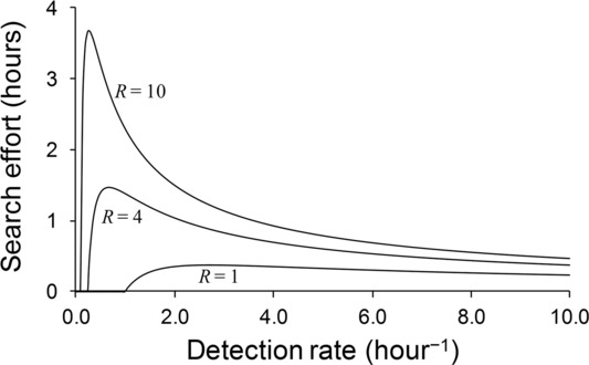
The search effort that minimizes the expected cost as a function of the detection rate (λ) for three different values for the expected benefit of detection (R).

Probability of acceptable outcome

The above analysis calculates the expected cost, but the actual cost will be typically different from that. In fact, the actual cost can be substantially different. Managers might be sensitive to the expected cost when averaging over many decisions. However, if a manager has only one site to consider, s/he might be more sensitive to the actual cost than the expected cost. In this case, the manager might be sensitive not just to the expected cost, but also uncertainty in that cost.

In this example, the manager will incur one of three actual costs that represent the instances when (1) the species is absent, (2) it is present and detected, and (3) it is present and undetected (Table1). A manager who is sensitive to uncertainty in the actual cost might aim to minimize the probability that the cost exceeds an acceptable threshold rather than aiming to minimize the expected cost.

Table 1.

The three possible costs incurred when searching for an invasive species, and the probabilities of incurring each

Outcome	Cost	Probability
Species is absent	x	1 − p
Species is present and detected	x + cc	p(1−exp[−λx])
Species is present and undetected	x + ce	pexp[−λx]

When the acceptable cost is less than the cost of management (T < c_c), any search effort up to the acceptable cost will minimize the probability that the total cost exceeds the threshold. Beyond this effort, the outcome would be deemed unacceptable; and further searching would not be undertaken. This seems an unrealistic scenario because presumably the managers would be willing to at least pay the cost of controlling the invasive species if it were found given they are prepared to search. Similarly, the scenario when T exceeds the escape cost of escape (c_e) also seems unrealistic because a manager would be prepared to accept the maximum possible cost of not detecting the species (c_e) and managing it when the species had escaped; in this case none or minimal search effort (up to T − c_e) would be optimal.

The nontrivial results occur when T lies in the interval [c_c, c_e]. In this interval, the probability that the cost exceeds T is minimized by setting x to T – c_c (Fig. 4). At this point the amount spent on survey (x) leaves an amount of c_c (from a conceptual budget of T) that is available to control the species if it is found; if survey effort x were greater than T – c_c, then survey and management costs would exceed the acceptable total cost T if the species were found. In words, the manager should search for the species to such an extent that sufficient resources remain available to manage the species if it is found.

Figure 4.

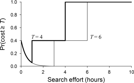
The probability of the costs exceeding an acceptable threshold (results shown for both T = 4 and 6 hours) when searching for an invasive species. The assumed parameters are a probability of presence (P = 0.4), a rate of detection (λ = 2 detections per hour), and costs of control when detecting the species (c_c = 3) and costs of escape when the species is present but remains undetected (c_e = 10).

This particular solution has an interesting feature; the survey effort that minimizes the probability that the costs exceed a threshold is independent of the probability of occurrence or the detection rate. Thus, uncertainty in these parameters will not impinge on the decision. The insensitivity to the probability of presence and detection rate is useful because managers simply need to know the costs (c_c and c_e) and the maximum acceptable cost (T) to determine the most robust search effort. This formulation even circumvents uncertainty about how detection probability changes with effort. Assumed to be exp[−λx] in this example, any declining function would lead to the same solution.

Stochastic dominance analysis

However, avoiding parameter and model uncertainty with this formulation comes at the cost of uncertainty about setting T. Managers will prefer lower costs, but a threshold below which a manager is happy with (but otherwise indifferent to) the costs, and above which she/he is unhappy (but is otherwise indifferent to costs) seems unlikely. Rather than examining a particular threshold, an alternative approach compares the cumulative distribution of the outcomes for each of the management options. Stochastic dominance analysis is a valuable framework for this comparison.⁵⁰ I provide an example of stochastic dominance analysis below (read Yemshanov et al.⁵¹ for a more detailed analysis relating to ecological management).

Outcomes when using stochastic dominance are typically expressed as benefits rather than cost C, so results here will be expressed as the benefit –C in which numbers that are more negative represent higher costs. Consider a choice between two different options—searching for 5 or 10 hours. The cumulative distribution of the benefit for each option is the probability that the actual benefit is less than the threshold (Fig. 5). Of these two options, searching for 5 hours is never worse than searching for 10 hours, and in some cases it is superior (for threshold costs of between 5 and 13 hours; Fig. 5A). Thus, searching for 5 hours is clearly superior to searching for 10 hours.

Figure 5.

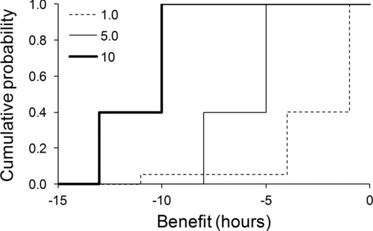
The cumulative distribution function of benefits (negative costs) when searching for 1, 5, or 10 hours for an invasive species (assuming λ = 2, c_c = 3, c_e = 10, and P = 0.4). Searching for 1 and 5 hours stochastically dominates searching for 10 hours at the first order. However, searching for 1 and 5 hours cannot be separated from each other at the first order because the functions cross.

In the parlance of stochastic dominance analysis, searching for 5 hours is first-order stochastic dominant over searching for 10 hours; preferring a first-order dominant strategy only requires the assumption that larger benefits are preferred to smaller benefits. Stochastic dominance can be expressed more formally in terms of cumulative distribution functions. Let F_i(z) be the cumulative distribution function of strategy i. Strategy A dominates strategy B if F_A(z) ≤ F_B(z) for all z, with a strict inequality for at least one value of z.

When the cumulative distributions of two strategies cross (Fig. 5), one strategy does not dominate the other at the first order. In this case, 1 hour of searching is preferable to 5 hours for benefits greater than −8 hours (costs <8 hours), but 1 hour is inferior (riskier) for larger cost outcomes. Separating these two options requires orders of stochastic dominance above the first. Each increase in order requires further assumptions about the preferences of the decision maker. If these preferences cannot be assumed, then the higher orders of stochastic dominance cannot be used to separate the options that are not separable with lower orders.

Determining second-order stochastic dominance requires the assumption that the manager prefers higher benefits (as for first-order stochastic dominance) and that his/her utility function is concave (the second derivative is everywhere negative). In this scenario, a concave utility function means a given increase in cost concerns the manager more when costs are already large than when costs are small. Essentially, this is a form of risk aversion, and is a reasonable assumption for many if not most managers.⁵⁰

If the assumption of a concave utility function is reasonable, then two options might be separated using second-order stochastic dominance by considering the integral of the cumulative distribution function. Option A dominates option B at the second order if 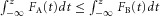for all z with at least one strict inequality.

Extending the comparison of 1 and 5 hours of searching (Fig. 5) to second-order dominance reveals that the integrals of the cumulative distribution functions cross (Fig. 6), showing that the options of searching for 1 hour and 5 hours cannot be separated using second-order stochastic dominance. The integrals of the cumulative distribution functions cross because searching for 1 hour is preferred for most outcomes, but is worse for the largest costs.

Figure 6.

The integral of the cumulative distribution function of benefits (negative costs) when searching for 1 or 5 hours for an invasive species (assuming λ = 2, c_c = 3, c_e = 10, and P = 0.4). Because the functions overlap, searching for 1 and 5 hours cannot be separated from each other at the second-order of stochastic dominance.

Separating management options with third-order stochastic dominance⁵² requires the assumption that the third derivative of the utility function of the manager is always positive. This assumption and those for higher-order dominance are less likely to be true for managers than the concavity assumption for second-order dominance, and understanding their practical significance is more difficult. Option A is third-order dominant over option B if for all z with at least one strict inequality. Note that the options of searching for 1 hour or 5 hours cannot be separated using third-order stochastic dominance.

Eliciting probabilities

When data are scarce or absent, probability distributions can be elicited from experts.⁵³ Clearly, such probabilities are prone to error. However, these errors are essentially analogous to the kinds of errors that might arise from probabilities estimated from data (for example, bias, imprecision, and context dependence). The relative magnitude of errors arising from data compared to errors arising from expert elicitation will depend on their relative reliability. However, at least some cases exist where expert judgments are more precise than estimates derived from limited data.⁵⁴

Procedures to account for the frailties of subjective judgement⁵⁵ are required when using experts to derive probabilities. These frailties include overconfidence (experts frequently underestimate uncertainty⁵⁶), anchoring (experts are often overly wedded to previous opinions), context dependence (linguistic uncertainty in questions must be minimized), motivational biases, and varying access to information.⁵⁵ Elicitation methods, however, can take advantage of factors that tend to reduce bias in the response of experts (e.g., feedback⁵⁷), resulting in structured processes for eliciting probabilities.⁵⁸

Portfolios

The previously described case where the optimal solution is not sensitive to the estimated probability (Fig. 4) is far from universal. Although equivalent cases exist (e.g., a reserve design problem where the decision is insensitive to uncertainty about extinction risk⁵⁹), assumed probabilities profoundly influence the choice among options in most cases. When elements of objectives are additive (e.g., minimizing the number of extinct species, which is the sum of species extinctions), epistemic uncertainty in the management objective is relatively tractable, and methods to deal with uncertainty in financial investment portfolios⁶⁰ can be adapted for conservation decision making.⁶¹

Further, when the management objective encompasses a sufficiently large number of additive components, one can rely on the central limit theorem such that the probability distribution of the objective will be approximately normal regardless of the distributions of individual components. However, problems with fewer components can be sensitive to the choice of distribution. For instance, Salomon et al.,⁶² when deciding about investing in managing survival and/or fecundity of a species, show that the choice of distribution for the management performance influences the best mix of the two management options. Difficulties arise when little or no information exists to inform the choice of distribution. Nonprobabilistic methods to decision making have developed largely due to such incertitude in, and sensitivity to, the choice of probability distributions.

Nonprobabilistic methods

Probabilistic descriptions of uncertainty help avoid linguistic uncertainty, because mathematical statements avoid ambiguity and vagueness and the context is also usually explicit. However, they can imply a degree of certitude that is unrealistic. Knight⁶³ distinguishes between measurable risk and unmeasurable uncertainty; probabilistic methods can be unsuitable for describing the latter, particularly for nonepistemic uncertainty.⁶⁴ Thus, various methods have been proposed to account for uncertainty that cannot be defined probabilistically.

Maximin

Wald's maximin model⁶⁵ considers the different possible states of nature and evaluates the performance of the different management options under all those states. One then searches across the possible states of nature, and finds the worst possible outcome for each action. For each action, one thus calculates the worst return that could be achieved. According to Wald's model, the most robust decision is to choose the action with the best “worst return.”

Wald's maximin model can be illustrated by the example of searching for an invasive species when the probability of presence of the species cannot be estimated. The two possible states of nature are that the species is absent or present, but we assume there is no basis for predicting the probability of presence. If the species is absent, the cost of management is simply equal to the cost of searching, x. If the species is present, then the manager will incur the control cost c_c plus the search cost x if the species is found; if the species remains undetected, the escape costs c_e and the search cost x will be incurred. With exp(−λx) being the probability that the species remains undetected, the expected cost when the species is present is exp(−λx)c_e + (1 − exp(−λx))c_c + x.

For all possible actions (all possible values of x), the worst outcome occurs when the species is present. Thus, the worst return is exp(−λx)c_e + (1 − exp(−λx))c_c + x. The value of x that achieves the best possible worst return is found by minimizing this function. Solving this gives Wald's maximin robust solution x_w = ln[(c_e−c_c) λ]/λ, which is the optimal search effort under the assumption that the species is present (i.e., assuming P = 1 in the probabilistic version).

Minimum regret

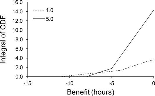
Wald's maximin solution tends to be very risk averse—it tends to extreme pessimism by design because it focuses on the worst possible outcome. An alternative is to frame the problem as one of minimizing the maximum regret in the decision.⁶⁶ In this case, the outcome for each action and each state of nature is compared to the best possible outcome for the corresponding state of nature. The difference in performance between the management decision and what would have been chosen if the true state of nature were known measures regret. One then determines the maximum possible regret (across different states of nature) for each action, and chooses the action with the smallest maximum regret.

In the search example, the best possible result, when the species is absent, would be to not search or manage, so the cost would be zero. Therefore, the regret when the species is absent is simply the search effort that has been expended unnecessarily, x (Fig. 7). When the species is present, the expected cost would be minimized by setting search effort to x_w = ln[(c_e−c_c) λ]/λ (as above for the maximin solution). Substituting this search effort into the expression for the expected cost gives the minimum possible expected cost when the species is present, which equals (1 + λc_c + ln[λ (c_e − c_c)])/ λ and provides the baseline against which regret is measured. Subtracting this minimum expected cost from the expected cost for a different search effort provides the regret when the species is present; following some algebraic manipulation, this can be shown to equal exp(−λx)r − (1 −λx + ln[λr])/ λ, where r = c_e − c_c is the extra cost of management following failed detection when the species is present. This regret (when the species is present) is positive when x = 0, declines to zero as x increases towards x_w, and then increases again with increasing x (Fig. 7).

Figure 7.

The regret when the species is absent (dashed line) and when the species is present (solid line). Regret measures the difference between expected cost for different search efforts and the expected cost that would be achieved if the presence or absence of the species were known. The search effort that minimizes the maximum regret is marked by the arrow, which is less than the search effort than minimizes the worst possible outcome (Wald's maximin solution is marked by the circle).

So now we have two measures of regret, depending on whether the species is present or absent; both are a function of the search effort x. Of course, we do not know which case holds—is the species present or absent? The principle of minimizing regret finds the search effort such that the larger of these two is minimized. In this case, the maximum regret is minimized when search effort equals ln (λr/[1+ln (λr)])/λ, for ln (λr) > −1; for smaller values of λr, the search effort that minimizes regret is x = 0. This search effort is less than Wald's (pessimistic) maximin solution that assumes the species is present (the worst possible outcome).

Scenarios

Considering the consequences of decisions under diverse alternative future scenarios⁶⁷ is similar to maximin. Diversity in the chosen scenarios can be increased by consulting a wide range of people with different perspectives. One can identify decisions that perform adequately over a wide range of scenarios. There are clear analogies with formal maximin and related methods, which could help assess performance of alternative management strategies under the different scenarios. Scenarios can share understanding among participants with different perspectives, and help understand major uncertainties and avoid surprises. Peterson et al.⁶⁷ document cases where scenarios have aided decision making in the face of uncertainty.

Info-gap decision theory

Ben-Haim^68,69 proposed info-gap decision theory as another way of dealing with cases where probabilities cannot be defined reliably. It has been used frequently to explore uncertainty in environmental management problems. Hayes et al.⁷⁰ counted more than 20 info-gap studies in ecology. While use of info-gap decision theory has increased, so have criticisms. I have published papers using info-gap decision theory,^71–74 but now I agree with critics that it overstates the level of uncertainty that it accommodates. Sniedovich^75–78 is a vocal critic, although some turns of phrase (e.g., referring to “voodoo decision making”) and his mathematical treatment might obscure the case in the eyes of many ecologists. Simultaneously, Sniedovich⁷⁸ argues that defenders of info-gap do not address his major criticisms, which essentially dispute the form of uncertainty analyzed by info-gap decision theory.⁷⁰

Info-gap can accommodate model uncertainty, but for the sake of simplicity I will restrict this discussion to parameter uncertainty. Info-gap decision theory requires initial values for uncertain parameters in the decision model. Then the analyst chooses a model of uncertainty by building an uncertainty interval around these initial values. For example, when considering the detection rate λ in the invasive search problem, an info-gap model sets an initial value . Then uncertainty around that parameter is defined by an interval, the width of which increases with a nonnegative parameter α. Thus, the interval could be [/(1+ α), (1+ α)], the range of which increases with α. I call this interval a multiplicative uncertainty model. The lower bound is defined to ensure that the detection rate is always positive. However, alternative models could be chosen; one with a different upper bound is [/(1+ α), + α], which I call an additive model. The choice is largely arbitrary, but as we will see, the choice influences the results.

Uncertainty in other parameters can also depend on α. For the extra cost of management following failed detection (r = c_e − c_c), we could use an additive uncertainty model for the upper limit [/(1+w α), + w α], or multiplicative model [/(1+w α), (1+w α)]. Here w defines how quickly the interval for r expands with α relative to the interval for λ. Alternative models could be used, including those with different models for the lower limit, but this set of models is sufficient for illustrative purposes.

Once the uncertainty model is defined, info-gap robustness is maximized by finding the strategy that allows α to be as large as possible while still achieving a required level of performance regardless of the values of the uncertain parameters within the uncertainty intervals. This is a reasonable goal—it finds the option that allows the parameter estimates to deviate as far as possible from the initial estimates, while still achieving an acceptable level of performance. This has analogies to the goal of maximizing the probability of achieving an acceptable level of performance. Info-gap results often depend on the choice of the initial estimate, the uncertainty model (which implicitly defines what far actually means) and the acceptable level of performance.

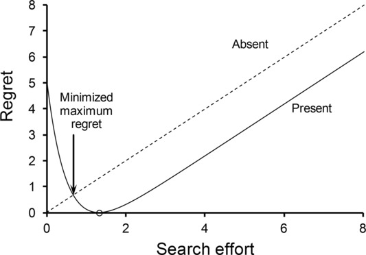
Using the info-gap model defined above for invasive species detection, we see that the most robust strategy depends on the choice of uncertainty model, and the values of , , and w (Fig. 8), illustrating a common result that the outcomes of info-gap analyses can be very sensitive to these choices. In the case of ignorance about the most appropriate choice, a manager would have no basis for this choice, so info-gap can only apply when we have a reasonable best guess. Without a reasonable best guess, a manager would have no basis to decide which uncertainty model and which best estimate (and hence, which curve in Fig. 8) would be most applicable, so info-gap decision theory could not help choose the most robust search effort. Sniedovich⁷⁶ notes that info-gap modeling is a form of local uncertainty analysis because it analyzes variation around particular parameter values; it is known as a stability radius model, a method that has existed since circa 1960,⁷⁸ decades before info-gap.

Figure 8.

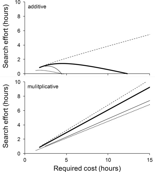
Search effort that maximizes info-gap robustness versus the required maximum cost for two different uncertainty models (additive and multiplicative) and four different combinations of the parameters (initial value for the extra cost of management following failed detection), (initial value for the detection rate), and w (the relative uncertainty in r and λ). The four sets of parameters are: = 7, = 2, w = 1 (thick line); = 7, = 1, w = 1 (thin line); = 7, = 2, w = 2 (dashed line); and = 3, = 2, w = 1 (dotted line). In all cases c_c = 1.

The common dependence of info-gap results on the chosen features of the info-gap model (e.g., see Fig. 8) mirrors a similar dependence that typically arises when using probabilistic models. Decisions based on probabilistic models often depend on the chosen distribution.⁶² Burgman and Regan⁷⁹ (p. 227) note that often probability distributions “cannot be guessed at reliably. Instead, it may be more expeditious to apply a horizon of uncertainty around a model, and ask to what extent is the rank of decisions stable under uncertainty.” However, info-gap analyses do not relieve analysts of equivalent guesses because analysts must choose from an infinite range of possible info-gap uncertainty models. Indeed, the basic features required to define a probability distribution can be thought of as an initial value (e.g., a median), and a model of uncertainty around that value (the probability distribution), which are broadly equivalent to the features of an info-gap model. Therefore, info-gap decision theory does not avoid the need to define the same types of attributes as required for probabilistic models.

This analogy with probabilistic models further emphasizes that info-gap models do not account for the type of uncertainty considered by Knight,⁶³ where we have no basis to choose a probability distribution. This is contrary to Ben-Haim's claim that info-gap models are suitable when probabilities cannot be defined reliably.^68,69 Instead, info-gap models help determine management actions that are robust to variation around an initial estimate. This form of analysis has proved useful in conservation decisions;⁷⁹ whether it deals with severe uncertainty (Sniedovich⁷⁶ says it does not) might be a matter of semantics.⁷⁹ However, the difficulties of using probabilistic methods in the face of substantial uncertainty are not avoided by substituting an uncertainty model where the choice of the substitute is similarly difficult and influential. Info-gap does not appear to solve the problem that it purports to, and this is the central criticism; not that it is unhelpful for local uncertainty analysis.

Conclusion

Methods to contend with uncertainty in conservation management decisions are increasingly used. The vast majority of methods account for epistemic uncertainty. Accounting for linguistic uncertainty is rarer, although methods also exist to account for this source of uncertainty.⁵⁵ Ignorance and indeterminacy continue to confound environmental management problems. These uncertainties arise in all aspects of decision making, including in objectives, knowledge about the system being managed, the efficacy of actions, and constraints. Analyzing scenarios^67,80 provides one mechanism to help address concerns about ignorance. While quantitative methods to account for uncertainty must aid decisions if the underlying models are sufficient approximations of reality, whether such models are sufficiently accurate has not yet been examined. Empirical evidence would be extremely valuable on how well quantitative methods account for uncertainty in conservation management decisions.

Conflicts of interest

The author declares no conflicts of interest.

References

- 1.McCarthy DP, et al. Financial costs of meeting global biodiversity conservation targets: current spending and unmet needs. Science. 2012;338:946–949. doi: 10.1126/science.1229803. [DOI] [PubMed] [Google Scholar]
- 2.Possingham H. Making smart conservation decisions. In: Orians GH, et al., editors; Soule ME, editor. Conservation Biology: Research Priorities for the Next Decade. Washington DC: Island Press; 2001. pp. 225–244. [Google Scholar]
- 3.Conservation Measures Partnership. Open standards for the practice of conservation. 2013. Version 3.0/April 2013.
- 4.Regan HM, Colyvan M. Burgman MA. A taxonomy and treatment of uncertainty for ecology and conservation biology. Ecol. Appl. 2002;12:618–628. [Google Scholar]
- 5.Skinner DJC, Rocks SA. Pollard SJT. A review of uncertainty in environmental risk: characterising potential natures, locations and levels. J. Risk Res. 2014;17:195–219. [Google Scholar]
- 6.Shaffer ML. Minimum viable populations: coping with uncertainty. In: Soule ME, editor. Viable Populations for Conservation. Cambridge, UK: Cambridge University Press; 1987. pp. 59–68. [Google Scholar]
- 7.Boyce MS. Population viability analysis. Ann. Rev. Ecol. System. 1992;23:481–506. [Google Scholar]
- 8.Burgman MA, Ferson S. Akçakaya HR. Risk Assessment in Conservation Biology. London, UK: Chapman and Hall; 1993. [Google Scholar]
- 9.IUCN. 2001. Gland, Switzerland IUCN Red List Categories and Criteria, Version 3.1.
- 10.Caughley G. Directions in conservation biology. J. Anim. Ecol. 1994;63:215–244. [Google Scholar]
- 11.Secretariat of the Convention on Biological Diversity. 2010. Montreal, Canada Global Biodiversity Outlook 3 , Secretariat of the Convention on Biological Diversity.
- 12.Runge MC. An introduction to adaptive management for threatened and endangered species. J. Fish Wildl. Manage. 2011;2:220–233. [Google Scholar]
- 13.Sanchirico JN, Springborn MR, Schwartz MW. Doerr AN. Investment and the policy process in conservation monitoring. Conserv. Biol. 2014;28:361–371. [Google Scholar]
- 14.Keeney RL. Gregory RS. Selecting attributes to measure the achievement of objectives. Oper. Res. 2005;53:1–11. [Google Scholar]
- 15.Polasky S, et al. Where to put things? Spatial land management to sustain biodiversity and economic returns. Biol. Conserv. 2008;141:1505–1524. [Google Scholar]
- 16.Hauser CE. McCarthy MA. Streamlining ‘search and destroy’: cost-effective surveillance for invasive species management. Ecol. Letters. 2009;12:683–692. doi: 10.1111/j.1461-0248.2009.01323.x. [DOI] [PubMed] [Google Scholar]
- 17.Beder S. Costing the Earth: equity, sustainable development and environmental economics. NZ J. Environ. Law. 2000;4:227–243. [Google Scholar]
- 18.Tisdell CA. Economics of Environmental Conservation. Cheltenham, UK: Edward Elgar Publishing; 2005. [Google Scholar]
- 19.Carpenter SR, Ludwig D. Brock WA. Management of eutrophication for lakes subject to potentially irreversible change. Ecol. Appl. 1999;9:751–771. [Google Scholar]
- 20.McCarthy MA. Possingham HP. Active adaptive management for conservation. Conserv. Biol. 2007;21:956–963. doi: 10.1111/j.1523-1739.2007.00677.x. [DOI] [PubMed] [Google Scholar]
- 21.Rout TM, et al. When to declare successful eradication of an invasive predator. Anim. Conserv. In press. [Google Scholar]
- 22.Regan T, et al. Optimal eradication: when to stop looking for an invasive plant? Ecol. Letters. 2006;9:759–766. doi: 10.1111/j.1461-0248.2006.00920.x. [DOI] [PubMed] [Google Scholar]
- 23.McCarthy MA. Red kangaroo (Macropus rufus) dynamics: effects of rainfall, harvesting, density dependence and environmental stochasticity. J. Appl. Ecol. 1996;33:45–53. [Google Scholar]
- 24.Burgman MA, Ferson S. Lindenmayer DB. The effect of the initial age-class distribution on extinction risks: implication for the reintroduction of Leadbeater's possum. In: Serena M, editor; Reintroduction Biology of Australian and New Zealand Fauna. Chipping Norton, Australia: Surrey Beatty; 1995. pp. 15–19. [Google Scholar]
- 25.Margules CR. Pressey RL. Systematic conservation planning. Nature. 2000;405:243–253. doi: 10.1038/35012251. [DOI] [PubMed] [Google Scholar]
- 26.McCarthy MA, Thompson CJ. Garnett ST. Optimal investment in conservation of species. J. Appl. Ecol. 2008;45:1428–1435. [Google Scholar]
- 27.Joseph LN, Maloney RF. Possingham HP. Optimal allocation of resources among threatened species: a project prioritization protocol. Conserv. Biol. 2009;23:328–338. doi: 10.1111/j.1523-1739.2008.01124.x. [DOI] [PubMed] [Google Scholar]
- 28.Baxter PWJ, et al. Accounting for management costs in sensitivity analyses of matrix population models. Conserv. Biol. 2006;20:893–905. doi: 10.1111/j.1523-1739.2006.00378.x. [DOI] [PubMed] [Google Scholar]
- 29.Chadès I, et al. General rules for managing and surveying networks of pests, diseases, and endangered species. Proc. Nat. Acad. Sci. U.S.A. 2011;108:8323–8328. doi: 10.1073/pnas.1016846108. [DOI] [PMC free article] [PubMed] [Google Scholar]
- 30.Chadès I, et al. When to stop managing or surveying cryptic threatened species. Proc. Nat. Acad. Sci. U.S.A. 2008;105:13936–13940. doi: 10.1073/pnas.0805265105. [DOI] [PMC free article] [PubMed] [Google Scholar]
- 31.Burnham KP. Anderson DR. Model Selection and Multi-model Inference: a Practical Information-theoretic Approach. New York: Springer-Verlag; 2002. [Google Scholar]
- 32.Probert WJM, et al. Managing and learning with multiple models: objectives and optimization algorithms. Biol. Conserv. 2011;144:1237–1245. [Google Scholar]
- 33.Holling CS. Adaptive Environmental Assessment and Management. Caldwell, New Jersey, USA: Blackburn Press; 1978. [Google Scholar]
- 34.Walters CJ. Hilborn R. Ecological optimization and adaptive management. Ann. Rev. Ecol. System. 1978;9:157–188. [Google Scholar]
- 35.Walters CJ. Adaptive Management of Renewable Resources. Caldwell, New Jersey: Blackburn Press; 1986. [Google Scholar]
- 36.Moore AL. McCarthy MA. On valuing information in adaptive management models. Conserv. Biol. 2010;24:984–993. doi: 10.1111/j.1523-1739.2009.01443.x. [DOI] [PubMed] [Google Scholar]
- 37.Grantham HS, et al. Delaying conservation actions for improved knowledge: how long should we wait? Ecol. Letters. 2009;12:293–301. doi: 10.1111/j.1461-0248.2009.01287.x. [DOI] [PubMed] [Google Scholar]
- 38.Nicol S. Chadès I. Which states matter? An application of an intelligent discretization method to solve a continuous POMDP in conservation biology. PloS One. 2012;7:e28993. doi: 10.1371/journal.pone.0028993. [DOI] [PMC free article] [PubMed] [Google Scholar]
- 39.Runge MC, Converse SJ. Lyons JE. Which uncertainty? Using expert elicitation and expected value of information to design an adaptive program. Biol. Conserv. 2011;144:1214–1223. [Google Scholar]
- 40.Wintle BA, Runge MC. Bekessy SA. Allocating monitoring effort in the face of unknown unknowns. Ecol. Letters. 2010;13:1325–1337. doi: 10.1111/j.1461-0248.2010.01514.x. [DOI] [PubMed] [Google Scholar]
- 41.Moore, et al. Estimating detection-effort curves for plants using search experiments. Ecol. Appl. 2011;21:601–607. doi: 10.1890/10-0590.1. [DOI] [PubMed] [Google Scholar]
- 42.Kouba, et al. Emerging trends for biobanking amphibian genetic resources: the hope, reality and challenges for the next decade. Biol. Conserv. 2013;164:10–21. [Google Scholar]
- 43.Bottrill, et al. Is conservation triage just smart decision making. Trends Ecol. Evol. 2008;23:649–654. doi: 10.1016/j.tree.2008.07.007. [DOI] [PubMed] [Google Scholar]
- 44.Bottrill, et al. Finite conservation funds mean triage is unavoidable. Trends Ecol. Evol. 2009;24:183–184. [Google Scholar]
- 45.Jachowski DS. Kesler DC. Allowing extinction: should we let species go? Trends Ecol. Evol. 2009;24:180. doi: 10.1016/j.tree.2008.11.006. [DOI] [PubMed] [Google Scholar]
- 46.Parr, et al. Why we should aim for zero extinction. Trends Ecol. Evol. 2009;24:181. doi: 10.1016/j.tree.2009.01.001. [DOI] [PubMed] [Google Scholar]
- 47.Polasky, et al. Decision-making under great uncertainty: environmental management in an era of global change. Trends Ecol. Evol. 2011;26:398–404. doi: 10.1016/j.tree.2011.04.007. [DOI] [PubMed] [Google Scholar]
- 48.Jaynes ET. Probability Theory: The Logic of Science. Cambridge, UK: Cambridge University Press; 2003. [Google Scholar]
- 49.McCarthy MA. Bayesian Methods for Ecology. Cambridge, UK: Cambridge University Press; 2007. [Google Scholar]
- 50.Levy H. Stochastic Dominance: Investment Decision Making Under Uncertainty. the Netherlands: Kluwer Academic Publishers; 1998. [Google Scholar]
- 51.Yemshanov D, et al. Mapping ecological risks with a portfolio-based technique: incorporating uncertainty and decision-making preferences. Divers. Distrib. 2013;19:567–579. [Google Scholar]
- 52.Whitmore GA. Third-degree stochastic dominance. Am. Econ. Rev. 1970;60:457–459. [Google Scholar]
- 53.Martin TG, et al. Eliciting expert knowledge in conservation science. Conserv. Biol. 2012;26:29–38. doi: 10.1111/j.1523-1739.2011.01806.x. [DOI] [PubMed] [Google Scholar]
- 54.Martin TG, et al. The power of expert opinion in ecological models using Bayesian methods: impact of grazing on birds. Ecol. Appl. 2005;15:266–280. [Google Scholar]
- 55.Burgman MA. Risks and Decisions for Conservation and Environmental Management. Cambridge, UK: Cambridge University Press; 2005. [Google Scholar]
- 56.O'Hagan A, et al. Uncertain Judgements: Eliciting Experts’ Probabilities. Chichester, UK: Wiley; 2006. [Google Scholar]
- 57.Wintle BC, et al. Improving visual estimation through active feedback. Methods Ecol. Evol. 2013;4:53–62. [Google Scholar]
- 58.Speirs-Bridge A, et al. Reducing overconfidence in the interval judgments of experts. Risk Anal. 2010;30:512–523. doi: 10.1111/j.1539-6924.2009.01337.x. [DOI] [PubMed] [Google Scholar]
- 59.McCarthy MA, et al. Designing nature reserves in the face of uncertainty. Ecol. Letters. 2011;14:470–475. doi: 10.1111/j.1461-0248.2011.01608.x. [DOI] [PubMed] [Google Scholar]
- 60.Markowitz H. Portfolio Selection: Efficient Diversification of Investment. Cambridge, MA: Blackwell; 1991. [Google Scholar]
- 61.McCarthy MA, et al. Resource allocation for efficient environmental management. Ecol. Letters. 2010;13:1280–1289. doi: 10.1111/j.1461-0248.2010.01522.x. [DOI] [PubMed] [Google Scholar]
- 62.Salomon Y, et al. Incorporating uncertainty of management costs in sensitivity analyses of matrix population models. Conserv. Biol. 2013;27:134–144. doi: 10.1111/cobi.12007. [DOI] [PubMed] [Google Scholar]
- 63.Knight FH. Risk, Uncertainty, and Profit. Boston: Hart: Schaffner & Marx, Houghton Mifflin Company; 1921. [Google Scholar]
- 64.Colyvan M. Is probability the only coherent approach to uncertainty. Risk Anal. 2008;28:645–652. doi: 10.1111/j.1539-6924.2008.01058.x. [DOI] [PubMed] [Google Scholar]
- 65.Wald A. Statistical decision functions which minimize the maximum risk. Annal. Math. 1945;46:265–280. [Google Scholar]
- 66.Savage LJ. The theory of statistical decision. J. Am. Stat. Assoc. 1951;46:55–67. [Google Scholar]
- 67.Peterson GD, Cumming GS. Carpenter SR. Scenario planning: a tool for conservation in an uncertain world. Conserv Biol. 2003;17:358–366. [Google Scholar]
- 68.Ben-Haim Y. Info-Gap Decision Theory: Decisions Under Severe Uncertainty. 1st ed. London, UK: Elsevier; 2001. [Google Scholar]
- 69.Ben-Haim Y. Info-Gap Decision Theory: Decisions Under Severe Uncertainty. 2nd edn. London, UK: Elsevier; 2006. [Google Scholar]
- 70.Hayes KR, et al. Severe uncertainty and info-gap decision theory. Methods Ecol. Evol. 2013;4:601–611. [Google Scholar]
- 71.Halpern, et al. Accounting for uncertainty in marine reserve design. Ecol. Letters. 2006;9:2–11. doi: 10.1111/j.1461-0248.2005.00827.x. [DOI] [PubMed] [Google Scholar]
- 72.Fox DR, et al. An info-gap approach to power and sample size calculations. Environmetrics. 2007;18:189–203. [Google Scholar]
- 73.McCarthy MA. Lindenmayer DB. Info-gap decision theory for assessing the management of catchments for timber production and urban water supply. Env. Manage. 2007;39:553–562. doi: 10.1007/s00267-006-0022-3. [DOI] [PubMed] [Google Scholar]
- 74.Rout TM, Thompson CJ. McCarthy MA. Robust decisions for declaring eradication of invasive species. J. Appl. Ecol. 2009;46:782–786. [Google Scholar]
- 75.Sniedovich M. Black swans, New Nostradamuses, voodoo decision theories, and the science of decision making in the face of severe uncertainty. Int. Trans. Oper. Res. 2010;19:253–281. [Google Scholar]
- 76.Sniedovich M. Fooled by local robustness. Risk Anal. 2012;32:1630–1637. doi: 10.1111/j.1539-6924.2011.01772.x. [DOI] [PubMed] [Google Scholar]
- 77.Sniedovich M. Fooled by local robustness: an applied ecology perspective. Ecol. App. 2012;22:1421–1427. doi: 10.1890/12-0262.1. [DOI] [PubMed] [Google Scholar]
- 78.Sniedovich M. Response to Burgman and Regan: the elephant in the rhetoric on info-gap decision theory. Ecol. App. 2014;24:229–233. doi: 10.1890/13-1096.1. [DOI] [PubMed] [Google Scholar]
- 79.Burgman MA. Regan HM. Information-gap decision theory fills a gapin ecological applications. Ecol. App. 2014;24:227–228. doi: 10.1890/12-1784.1. [DOI] [PubMed] [Google Scholar]
- 80.Nicholson E, et al. Making robust policy decisions using global biodiversity indicators. PloS One. 2012;7:e41128. doi: 10.1371/journal.pone.0041128. [DOI] [PMC free article] [PubMed] [Google Scholar]