

Abstract
Spectral domain optical coherence tomography (SD-OCT) is a high resolution imaging technique that generates excellent contrast based on intrinsic optical properties of the tissue, such as neurons and fibers. The SD-OCT data acquisition is performed directly on the tissue block, diminishing the need for cutting, mounting and staining. We utilized SD-OCT to visualize the laminar structure of the isocortex and compared cortical cytoarchitecture with the gold standard Nissl staining, both qualitatively and quantitatively. In histological processing, distortions routinely affect registration to the blockface image and prevent accurate 3D reconstruction of regions of tissue. We compared blockface registration to SD-OCT and Nissl, respectively, and found that SD-OCT-blockface registration was significantly more accurate than Nissl-blockface registration. Two independent observers manually labeled cortical laminae (e.g. III, IV and V) in SD-OCT images and Nissl stained sections. Our results show that OCT images exhibit sufficient contrast in the cortex to reliably differentiate the cortical layers. Furthermore, the modalities were compared with regard to cortical laminar organization and showed good agreement. Taken together, these SD-OCT results suggest that SD-OCT contains information comparable to standard histological stains such as Nissl in terms of distinguishing cortical layers and architectonic areas. Given these data, we propose that SD-OCT can be used to reliably generate 3D reconstructions of multiple cubic centimeters of cortex that can be used to accurately and semi-automatically perform standard histological analyses.
Introduction
Optical Coherence Tomography (OCT) is an optical technique that provides high resolution cross sectional imaging as well as 3D reconstructions of up to several hundred microns in depth of biological tissues. Huang and colleagues introduced OCT in 1991 for studying the retina and the coronary artery (Huang et al., 1991). OCT is analoguous to ultrasound imaging as it measures the backscattered light of the sample, and is sensitive to differences in the refraction index in tissue. Hence, cell bodies and myelinated fibers offer high intrinsic contrast compared to the extracellular matrices (Ben Arous et al., 2011; Srinivasan et al., 2012). The ability to visualize both cytoarchitectonic and myeloarchitectonic structure in the 3D blocks of tissue may have a significant impact on the fields of brain mapping, histology and neuropathology. Assayag and colleagues utilized OCT for brain tumor diagnosis and qualitatively compared it with histology (Assayag et al., 2013). OCT enables us to image histological architectural characteristics found in normal brain tissue (neurons, fibers and vasculature), and has been used to distinguish tumors (i.e. meningiomas from heman-giopericytoma, choroid plexus papilloma and diffusely infiltrated gliomas).
Traditional histology has provided the ground truth for validation in structural neuroimaging. The validation between ex vivo MRI and histochemical staining has helped to establish improved estimates of cortical boundaries (Fischl et al., 2009; Augustinack et al., 2005, 2013; Geyer et al., 2011; Caspers et al., 2012; Amunts et al., 2013), pathological composition (Bö and Geurts, 2004; Nagara et al., 1987) and provide a better understanding of ex vivo image contrast (Eickhoff et al., 2005). With standard histological methods, tissue sections undergo a tremendous amount of physical manipulation (i.e. sectioning, mounting) as well as chemical changes (i.e. dehydration, staining). Due to the integrity differences of human tissue and the practicality of tissue handling, deformations and damages inevitably occur during traditional histological staining. The OCT method offers a new avenue for brain mapping that acquires architectural-level information on blocks of tissue as opposed to excised tissue slices. OCT does not require staining and it makes use of the intrinsic properties of the neurons and fibers to generate contrast. The OCT method is contact free with less physical handling, which may lead to better registration between ground truth histology and imaging.
In this report, we compared traditional Nissl staining and OCT in ex vivo samples. We quantitatively analyzed the registration between OCT and blockface photography as well as between OCT and Nissl stained section. We investigated the lamina in temporal isocortical samples using line profiles and quantitatively compared the accuracy and reliability between OCT and Nissl. Here, we provided evidence that OCT provides information that is comparable to Nissl staining and we discuss the advantages of each method.
Methods and Materials
Spectral Domain Optical Coherence Tomography
OCT uses low coherence interferometry and employs a light source with low temporal coherence (i.e. a broad spectral bandwidth). The light source is split into two arms: the reference arm, which is reflected on a mirror, and the sample arm, which illuminates the sample. The light from the arms is recombined to measure the interference between the reference and the sample light that can only occur when their path lengths are matched within the coherence length of the source (within several micrometers). When the technique was first developed, it was engineered such that the reference mirror moved to scan the sample axially, and was known as Time Domain OCT (TD-OCT). However, a more effective way to perform tomography, with higher sensitivity and faster scan rate, is to use the spectral variations of the signal recorded by a spectrometer, a technique known as Spectral Domain OCT (SD-OCT) (Fercher et al., 1995; Yaqoob et al., 2005). With this method, the reference mirror is immobile and depth information is encoded in the spectral variations using the Fourier relation. An x-y galvanometric scanner is used to scan the sample laterally and a 3D volume is recorded. The apparatus is further improved to achieve higher resolution by inserting an objective lens into the object arm to focus the light on the sample; this is referred to as Optical Coherence Microscopy (OCM). The depth and lateral resolutions are independent. The depth resolution is linked to the coherence length of the light source; it improves as the spectral bandwidth of the light increases. The lateral resolution is related to the numerical aperture (NA) of the objective lens. The larger the NA is, the higher the lateral precision. The depth of focus is also dependent on the NA, and decreases as the NA increases. The apparatus used for this study has been described in detail in (Srinivasan et al., 2012) and is illustrated in Fig. 1.
Figure 1.
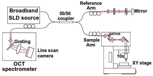
Optical coherence microscopy schematics. See text for more details.
The broadband light source used in this study was a superluminescent diode (SLD) with a center wavelength of 1310 nm and a full width at half maximum of 170 nm, which yielded an axial resolution of 4.7 μm in air (3.5 μm in tissue). In the sample arm, a 10x water immersion objective (Zeiss N-Achroplan 10x W, NA 0.3) was used, which produced a lateral resolution of 3 μm in tissue, a depth of focus of about 30 μm and a field of view of 1.5 mm × 1.5 mm. The spectrometer consisted of a grating and a 1024 pixel InGaAs line scan camera (Thorlabs Inc, Newton, New Jersey, USA). Each acquired spectrum, called A-scan, represented the depth profile over 1.5 mm of the tissue sample for a given (x,y) postion. Two galvo mirrors allowed us to scan the sample spatially over the whole field of view. Each data acquisition consisted of a 3D volume of 512 × 512 × 512 pixels. The brain tissue was adhered with glue (Instant Krazy Glue, Elmer’s Products, Inc, Westville, OH, USA) to a glass petri dish and immersed in water. The sample rested on a manual X-Y stage (Optometrix, 1 inch displacement) allowing translation in both directions and imaging tiles over several square centimeters.
Each data volume was first processed independently. The 2D average intensity projection (AIP) over 400 μm depth from the surface was assessed for each 3D volume to visualize the laminar structure of the cortex. The whole sample was reconstructed by stitching the individual images together using a Fiji plug-in based on the Fourier shift theorem (Preibisch et al., 2009). Approximate coordinates were used as input to facilitate the stitching. A total variation filtering and an intensity adjustment were performed on each tile to improve image quality (Gilboa et al., 2003; Rudin et al., 1992).
Tissue samples
Five temporal isocortical samples were obtained from the Massachusetts General Hospital Autopsy Suite (Boston, MA). All brain samples were fixed by immersion in 10% formalin for at least two months, until thoroughly fixed. The sample blocks included Brodmann areas 36, 20, 21, 22 and sometimes 41 and were typically 1 cm thick. These areas represent the lateral half of the temporal lobe and the isocortical tissue type. Functionally, areas 36, 20, 21 and part of 22 carry out visual associative processing while the upper bank of the superior temporal sulcus acts as a multimodal area, and area 41 consists of primary auditory cortex. The demographics of our sample set were: 65.5 ± 16.9 year old, that ranged from 45 to 86 years old; two cases were males, two females and one case had no demographic information. The post-mortem interval did not exceed 24 hours. Four cases studied were control brains and did not contain neurological deficits but the fifth case was pathologically diagnosed as mild Alzheimer’s disease.
Tissue processing and histology
To create a flat surface as required for optimal OCT acquisition, we first sectioned the 1 cm thickspecimen block with a sliding freezing microtome (standard equipment for large human sections, but a vibratome may be used) for the histology studies before we acquired the OCT data, leaving approximately 0.5 cm thickness for the tissue block. This thickness is arbitrary and no thickness limit is imposed by the OCT technique other than the space available below the objective. This flatfacing created an ultra flat landscape for the tissue face that helps improve the data acquired with OCT, by providing a homogeneous illumination when the light is focused under the surface. Typically, we sectioned forty slices at 50 μm of each case for histological staining and photographed each blockface before each slice was sectioned; blockface images served as a guide while mounting the tissue and as a ground truth in geometry for the registration. The free floating tissue sections were mounted onto gelatin dipped glass slides with a paintbrush and stained for Nissl substance on every fifth section. Our Nissl staining protocol has been previously described (Amunts et al., 1999; Zilles et al., 2002; Augustinack et al., 2005), and we briefly outline it here. Once dry, the unstained slides were treated in a series of solutions for Nissl staining: defatting (20 minutes in ChCl3:ethanol (EtOH) [1:1], 3 minutes in 50% EtOH, 3 minutes in double distilled water (ddH20)), pretreatment (1 minute in acetic acid:acetone:dd H2O:100% EtOH [1:1:1:1] and 1 minute ddH20), staining (5 minutes in buffered thionin) and finally dehydrated (in ddH20, 70% EtOH (twice), 95% EtOH (twice), 100% EtOH (twice) and cleared in xylene (twice)). Slides were then coverslipped with Permount (Fisher, Fairlawn, NJ).
The stained slices were evaluated on an 80i Nikon Microscope (Microvideo Instruments, Avon, MA) under low and high power magnification. The slides were photographed with a Canon EOS Digital Rebel XT (8 megapixels) with a 50 mm lens while illuminated with a Dolan Jenner light box (Boxborough, MA). Once photographed, the digitized images were optimized for contrast and tone (background substraction and auto contrast with the freeware Gimp1).
Registration
Next, the OCT images were registered to the histological slides, to compare the information content of the two modalities. To construct an affine registration between the OCT and the histology image, we employed a statistically robust approach described previously (Reuter et al., 2010). We specifically used an extension that transfers the robust and inverse-consistent approach for mono-modal image registration to the multi-modal setting by extracting a modality invariant image representation based on local entropy estimation for both modalities (Wachinger and Navab, 2012). Robust registration of entropy images allows the algorithm to reduce the influence of ‘outliers’, such as artifacts, in the images and can yield highly accurate registrations even in the presence of differences (e.g. different background segmentations or croppings). This method is also used to register both modalities to the blockface image to evaluate the distortions introduced by processing and imaging techniques of the tissue. We define distortions as tissue rips, tissue overlap or widening of gaps between gyri. In theory, it is possible to section and hand mount tissue so that there are no distortions of any kind. However, aging processes, post mortem interval, immersion fixation, the large size of the tissue samples and even possibly cause of death can compromise the integrity of human tissue. Thus, sectioning artifacts and mounting errors do occur due to the above mentioned reasons. The term distortion also includes the missing pieces of tissue that occasionally get removed while handling the tissue sample throughout the experimental procedures. In spite of precautions taken to avoid distortions during the tissue processing, artifacts cannot be avoided completely.
Manual labeling and profiles
Each modality was manually labeled independently by two observers using Freeview, a visualization tool included in FreeSurfer2, a brain imaging software package developed and supported by the Athinoula A. Martinos Center for Biomedical Imaging at Massachusetts General Hospital. Several landmarks were labeled. The gray/white matter boundary (GWB), the pial surface (PS) and selected cortical layers (CL). We labeled the most distinguishing lamina in each respective cortex. The cortical layers that were labeled may be different in each cortical area. For example, layer III (except on one case), IV and V were drawn on both Nissl and OCT images. For two sample cases, layer II was labeled and for one tissue sample, two cell free zones were drawn as well. We did not label layer VI due to the closeness to layer V and the GWB. Profile lines were constructed by solving the Laplace equation with appropriate boundary conditions (Jones et al., 2000). A Dirichlet condition of zero and one was specified on GWB and PS, respectively. The open ends were connected and a Neumann boundary condition of zero derivative normal to the boundary was specified. The Laplace equation was then solved on a refined pixel grid. Profile lines were computed by sampling the mid-level curve equidistantly and following the gradient up and down into the pial and white matter boundaries.
Results
OCT contrast
The depth profile acquired by OCT depends on the optical properties of the tissue (Wang et al., 2011). The light intensity exponentially decreases in the tissue with a decay rate that depends on the tissue attenuation coefficient. Gray matter and white matter exhibit significant differences in attenuation, higher for the white matter than for the gray matter. Futhermore the reflectivity of the fibers also depends on their orientation. Fibers that lie parallel to the surface show a higher reflectivity. The more oblique the fibers are relative to the surface, the lower the overall reflectivity. To investigate which optical parameters would best visualize cortical lamina, we evaluated the attenuation coefficient and the reflectivity. We downsampled each volume by averaging the depth profiles over 15 × 15 μm2 areas. For each mean profile, the focus depth was determined and a linear fit was applied to the logarithmic profiles over 150 μm starting 30 μm deeper than the focus. The slope corresponds to the attenuation coefficient and the intercept to the reflectivity. Fig. 2A shows the attenuation coefficient for a temporal isocortex sample. The white matter has a higher attenuation coefficient than the gray matter, which permits a good segmentation of brain tissue. Within the gray matter, a laminar structure was observed and resembled the cytoarchitecture obtained by Nissl staining. Fig. 2B illustrates the intercept of the linear model fitted to the log-transformed depth profile. Fig. 2B shows that the gray matter has an overall homogenous reflectivity, but a subtle laminar contrast can be observed. In contrast, the white matter has a heterogenous intensity showing the various fiber orientations relative to the surface. Brighter areas (e.g. white arrow in Fig. 2B) indicate fibers parallel to the surface. For more oblique fibers, the intercept value diminished and can even be lower than observed in the gray matter (e.g. black arrow in Fig. 2B). One simple and effective means to combine attenuation and reflectivity into a single image is to compute the AIP over the 400 μm that light penetrates the tissue, followed by stitching, filtering (total variation filter (Gilboa et al., 2003; Rudin et al., 1992)) and intensity adjustment (Fig. 2C). The gray matter appears brighter than the white matter due to its lower attenuation coefficient, similar to Fig. 2A. The laminar structure of the cortex is clearly visible. The heterogeneity of the fiber orientations in the white matter is also conserved and agrees with the reflectivity image Fig. 2B. For this study, we will focus on the gray matter, but we note that SD-OCT contains significant useful information on the location, degree of myelination and orientation of white matter fibers as well. In order to further improve the laminar contrast in the cortex, each image tile was first filtered and intensity adjusted, and then stitched together to create the whole sample image. As shown in Fig. 2D, this procedure greatly reduced the heterogeneity in the white matter, while enhancing the laminar contrast in the cortex. We therefore used this data processing (tile filtering before stitching) for the remainder of this study.
Figure 2.
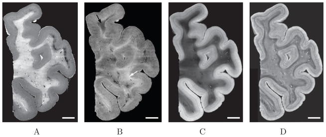
Four panels illustrate the same isocortical sample yet imaged with different contrasts. A: attenuation coefficient image, B: reflectivity image (the arrows showing different fiber orientations, white for parallel to the surface and black for more oblique fibers), C and D represent AIP images but different protocols were performed. C: the tiles are first stitched together, then the whole image is improved (filtering and intensity adjustment). Each tile is first improved to emphasize on the laminar structure of the cortex, then they are stitched together to reconstruct the whole volume. Note the improvement for the white matter in C and the cortical ribbon in D. Scale bar: 5mm
Qualitative comparison between Nissl stain and OCT
For each isocortex sample, we qualitatively compared the blockface image of the sample, the Nissl stain and the OCT images. Fig. 3 shows the three images obtained for one case. The distinction between gray matter and white matter was evident in all three modalities. We observed that the Nissl stain and OCT images showed an inverse contrast relative to one another (Fig. 3D). In the histology stained section (Fig. 3B), the Nissl substance indicates the presence of neuronal cell bodies and thus cell dense areas of the cortex are dark and highlight laminar structure while the white matter remains relatively unstained. Conversely, in the OCT image (Fig. 3C), the overall gray matter appears lighter than the white matter. Even though the myelinated fibers highly backscatter the light, it does not penetrate the white matter as well as the gray matter as the attenuation coefficient for white matter is higher, which leads to a lower intensity when averaged over several hundreds of microns in depth. The distortions (defined as rips, overlaps and relative position of the gyri) observed on this sample were mainly due to the sectioning, mounting and dehydration (Fig. 3B, arrows). For example, we observed on the Nissl stain (Fig. 3B) that one of the gyri was split (green arrow). In addition, a gyrus was positioned with an overlapping area (red arrow). Fewer distortions were observed on the OCT image because the data was collected from the tissue block prior to sectioning, diminishing the need for the cutting, mounting and staining that is required before imaging in traditional histological processes.
Figure 3.
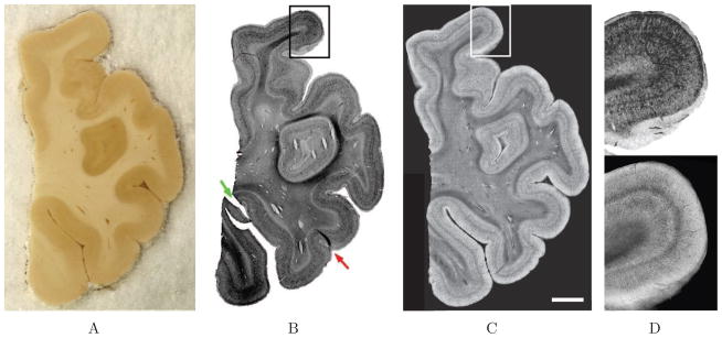
A: Blockface, B: Nissl stain, C: OCT images of one of the isocortex samples and D: comparison of contrast on the boxed region (top: Nissl and bottom: OCT). Scale bar: 5 mm.
Quantitative registration to the blockface
The blockface images provided the ground truth of the tissue geometry. We registered both the Nissl stain and the OCT image to the blockface photography. Once registered, all three images were binarized and overlaid using Matlab (The MathWorks, Inc., Natick, MA, USA) to assess the overlapping areas between the blockface image and both Nissl section and OCT image. Fig. 4A shows the registration of a sample case. Fig. 4A illustrates overlapping regions in white and the non-overlapping regions in red for the blockface image, in yellow for the Nissl stain (left image), and green for the OCT image (right image). This example reveals that, for the Nissl stained sections, the geometry of the gyri was not preserved during mounting, which is not the case in the OCT image since the data were acquired on the block tissue directly. The registration error for the Nissl stain is larger than for the OCT (Fig. 4A, white arrows). The overlapping area between the Nissl stain and the blockface image was 94.6 % of the true area whereas the overlapping area with OCT was 99.1%. Fig. 4B shows similar results for three other cases.
Figure 4.
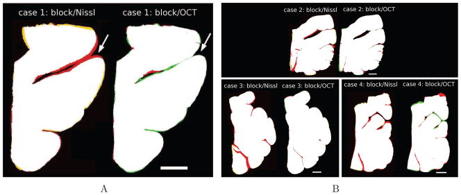
A: Blockface (red) registration with: Nissl stain (yellow) on the left and OCT image (green) on the right for one sample case; the overlap region is in white. B: Similar results for other cases. Red, yellow, and green represent the non-overlapping regions in blockface, Nissl and OCT, respectively. Scale bar: 5 mm.
Quantitative registration between modalities
To achieve accurate colocalization of the laminar structure on Nissl and OCT, registration is a critical step. The OCT and the Nissl stain images were registered to one another to evaluate cortical landmarks but also to highlight distortions (i.e rips, overlap, sulcal widening). Fig. 5 shows the registration error between the histology slices and the OCT image, with the Nissl stained tissue shown in red, the OCT image in yellow and the overlap of both modalities in white. The algorithm achieves a good overall registration. However, a few discrepencies were observed. For example, Fig. 3B shows one of the Nissl stained samples where the top part is detached (green arrow) and is then not mounted in the same position as it appears in the blockface photo (Fig. 3A), which induces registration errors (Fig. 5A, green arrow). Moreover, during the experimental procedures, the samples were handled multiple times, which resulted in missing pieces of tissues, as can be observed on Fig. 5B (green arrow). Nevertheless, the advantages of the robust approach are evident in this figure, in which the vast majority of the boundaries are well-registered with only isolated inaccuracies that do not reduce the quality of the overall alignment.
Figure 5.

Registration errors between histology and OCT for two different samples: Nissl stained slice (red), OCT (yellow) and overlap (white). Note: registration errors in red and yellow.
Laminar Labeling
A Nissl stained section provides cytoarchitectural information determined by the presence or absence of cortical laminae, as well as neuronal density, size and shape in a given area. The laminar labeling on both images is intensity-based and was performed on digital images independently for the two modalities. Qualitatively, we labeled the most visually distinguishable lamina throughout the sample. GWB and PS were also labeled. One example is shown in Fig. 6, for the Nissl stain (Fig. 6A) and the OCT (Fig. 6B) images. From the manual labeling, we solved the Laplace equation to generate profile lines (Fig. 7). The cortical thickness and the distance between layers in the two-dimensional plane were then measured using the profile lines. Because the human cerebral cortex has a complex 3D geometry, the sectioning plane often exhibits intricate structures. When the blocking and sectioning is performed perpendicular (or close to perpendicular) to the PS, the profile lines appear homogenously distributed (Fig. 7A). Conversely, when the cortical ribbon is far from perpendicular to the PS (i.e. oblique), some complex structures appear such as emerging or disappearing gyri (Fig. 6A, black arrow) and oblique gyri (Fig. 7B, box). Thus, the profile lines were not homogenously sampled in those particular regions and their laminar structures were more complicated to assess, both in the histological slices and the OCT images. Note that this is one significant potential advantage of OCT - the ability to analyze the cortex in 3D instead of 2D.
Figure 6.

Manual labeling of the cortical landmarks on co-registered Nissl stain (A) and OCT images (B). The drawn lines are the PS (magenta), the GWB (red) and the differents CL: layer II (dark blue), layer III (cyan), layer IV (green) and layer V (yellow). Scale bar: 5 mm.
Figure 7.
Profile lines generated for parts of two different samples on the Nissl stained slices. Red color in B is due to density of lines. Inset box shows an oblique gyrus - not fully formed in this slice. Scale bars: 2 mm.
Inter observer reliability
In this section we report on the reliability of the manual labeling. Two independent observers (Obs1 and Obs2) drew (i) lines on both modalities (Mod), the Nissl stained and the OCT images. The Haussdorff distance and the median minimal distance were evaluated between the corresponding lines i drawn by the two observers for each modality and .
For notational conciseness let and . Then the distances are defined as:
where d(x, y) is the distance matrix between X and Y and med represents the median.
The goal was to assess whether there were significant differences in labeling between observers with respect to the modality. A Wilcoxon signed rank test was performed to compare them for each of these three parameters. The lines have been classified into three groups: those corresponding to the GWB, to the PS and to the various cortical layers (CL). The results are shown on Fig. 8.
Figure 8.

Statistical analysis for the inter-observer reliability. A: the Haussdorff distance and B: the median minimal distance with respect to the modalities (Nissl and OCT) and the line groups (GWP, PS, CL). The red horizontal line within each box is the median, the edges of the box are the 25th and 75th percentiles, the error bars extend to the most extreme data points not considered outliers, and outliers are plotted individually as red + signs. The results of the Wilcoxon signed rank test is shown above the bracket by *, if p <= 0.05.
The GWB and PS lines did not exhibit a significant difference for those three parameters. For the CL lines, there were differences for the median minimal distance; however the p-values was only marginally significant at 0.026. The Hausdorff distance did not show any significant difference in the labeling between observers with respect to the image modality. Moreover, Fig. 8 shows that, as expected, the PS was the easiest to label, with the highest accuracy and reproducibility (i.e. smallest median minimum distance (red line) and smallest standard deviation), followed by GWB, which was easily detectable due to the change in intensity on both modalities and finally, labeling the CL lines was more challenging, as the middle of a cell dense or cell-poor layer has to be defined.
Inter modality reliability
Since the registration has some local errors due to intrinsic tissue quality and distortions induced during the histological protocol, overlaying both sets of lines for direct comparison is not ideal unless some adjustments are made for distortions. To compare the localization of the layers within the cortical ribbon, we projected the labeled lines drawn on the Nissl stained images onto the OCT images. To accomplish this, the displacement vectors between the gray/white matter boundaries (dGWB) of both modalities, as well as the displacement vectors between the pial surfaces (dPS), were first calculated. Then, the distance between the gray/white matter boundary and the layer i relative to the total cortical thickness was calculated using the profile lines and noted as ai. To remap the Nissl CL line to the OCT space, we used a bilinear weighting depending on the distance to the surfaces (GWB or PS) as follows:
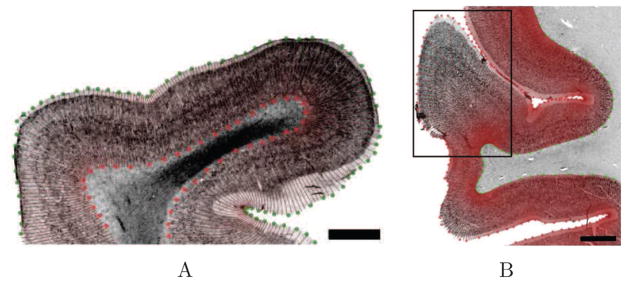
where is the projected histology layer line i in the OCT space. Two examples of mapping the Nissl CL lines into the OCT space are represented on Fig. 9. Fig. 9A and 9C show the original histology CL lines (+) overlaid on the OCT CL lines (○) while Fig. 9B and 9D show the projected histology CL lines on top of the OCT CL lines and image. On Fig. 9A, there is a large difference between the line on the right gyrus due to a mispositioning of the tissue during hand mounting as the PS lines suggest (magenta lines). After mapping the Nissl CL into the OCT space (Fig. 9B), the difference was largely reduced. Fig. 9C shows that the GWB is badly registered (red lines). The red lines in the fundus differ greatly between C and D. By mapping the histology lines onto the OCT space, we show an improved agreement between the two sets of lines (Fig. 9D).
Figure 9.

Two examples of the mapping of the Nissl lines to the OCT space (top and bottom). A and C: original Nissl (+) and OCT (○) lines. B and D: projected Nissl lines onto the OCT space (+) and the OCT lines (○). Scale bars: 5 mm for A and B and 2 mm for C and D.
Fig. 10 shows the statistical analysis of mapping the histology layer lines onto the OCT space. The Hausdorff distance (Fig. 10A) and the median minimum distance (Fig. 10B) were calculated: first between the OCT CL lines and the original histology lines (Orig), then between the OCT CL lines and the projected histology lines (Proj). A Wilcoxon sign rank test was also performed and showed a significant difference in the median minimum distance but not significant in the Hausdorff distance. The results are displayed above the bracket (** if p <= 0.01). The Haussdorff distance does not show significant difference with respect to the sign rank test, but the median Hausdorff distance (red line) was reduced by 30%, (from 0.951mm to 0.658mm). The median minimum distance showed a significant difference, with a p-value of 5.9e−3. The median minimum distance was reduced by 26%.
Figure 10.
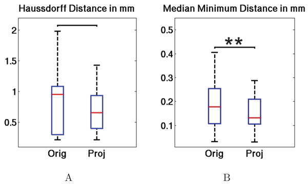
Statistical analysis of the mapping between the OCT CL lines and the original Nissl CL lines (Orig) or the projected Nissl CL lines (Proj). A: the Hausdorff distance, B: the median minimal distance. The red horizontal line within each box is the median, the edges of the box are the 25th and 75th percentiles, the error bars extend to the most extreme data points not considered outliers. The results of the Wilcoxon signed rank test are shown above the bracket by ** if p <= 0.01, and nothing if no significant difference).
Layer positions in the cortical ribbon
A factor in the assessment of the cortical boundaries is the relative positions of the different layers within the gray matter. For each sample, we computed the distance between GWB to the CL lines. The projected Nissl lines mapped onto the OCT images were used for the comparison with the OCT data. Fig. 11 shows results for two different tissue samples. The outcome measures for the Nissl stains are symbolized by + and the OCT ones by ○. The high peaks on both graphs are due to complex structures such as gyral pattern of the human brain (e.g., oblique section of the gray matter and emerging or disappearing gyrus) that are an artifact of this type of 2D analysis.. Qualitatively, the thicknesses are in good accordance. The Pearson’s correlation ρ between the corresponding lines for both modalities was calculated for each sample, as well as their p-value. The mean Pearson’s correlation was ρ=0.84 ± 0.16 with a very small p-value.
Figure 11.

Thickness from GWB to the CL lines for the Nissl stain (+) and the OCT (○). Data assessed for two cases.
Discussion
While structural brain mapping has improved with high resolution ex vivo MRI and histological validation, the resolution and contrast of MRI has limits that constrain our ability to visualize features in association cortices that typify homotypic cortex, even ex vivo. Refined localization of brain areas is critical for application to diseases such as autism, schizophrenia and Alzheimer’s disease. Although cortical segmentation and in vivo biomarkers have been developed, cytoarchitectural-level detail is difficult to obtain with MRI, particularly the subtle cytoarchitectural differences among association areas. Histology validation has linked ground truth cellular pattern with probabilistic whole-brain maps (Amunts et al., 1999; Schleicher et al., 1999; Amunts and Zilles, 2001; Fischl et al., 2008, 2009; Augustinack et al., 2013). However, human histology is labor intensive and leads to irremediable deformations due to blocking, cutting, mounting and staining, which render registration across slices and to other modalities difficult (Ceritoglu et al., 2010; Reuter et al., 2010; Augustinack et al., 2010; Reuter et al., 2012).
In this study, we compared OCT with traditional Nissl staining in 5 cortical samples. We analyzed the two modalities qualitatively and quantitatively, registered each modality to the blockface images and to each other (Nissl and OCT). We manually labeled cortical landmarks (mainly layers III, IV and V) to evaluate the validity of OCT with respect to the ground truth Nissl staining. Median minimum distance and Hausdorff distance served as outcome measures. Finally, we projected Nissl lamina lines onto the OCT to show intermodality agreement (or correspondence).
In this paper we have shown that OCT yields similar and in some instances improved results for cortical landmarks or laminae relative to standard histology. OCT has several advantages over traditional Nissl staining. First, OCT is a three dimensional imaging technique. Imaging cortical depth is a significant improvement over traditional tissue methods. In this paper, en-face projections of the average intensity over 400 μm depth were performed on each acquired volume and the whole sample reconstructed by stitching the images together, but in the future we intend to construct full 3D OCT volumes and implement analysis algorithms that take advantage of the full 3D representations. Second, traditional histology is a time consuming and labor intensive process. The tissue must be sectioned, hand mounted and stained. OCT relies on intrinsic optical contrast: the blockface is directly imaged. While OCT is also labor intensive, the whole OCT imaging process can be automated in the future. Third, contrary to other light microscopy techniques (Wilt et al., 2009; Chung et al., 2013) which require histochemical dyes to label the cells or the fibers, like two-photon microscopy (Denk et al., 1990; Helmchen and Denk, 2005), OCT does not require the use of stains or dyes. Finally, in addition to cytoarchitecture, OCT can also assess the myeloarchitecture of the cortex since myelinated fibers highly backscattered the light. Myeloarchitecture has been demonstrated in rodent brains (Wang et al., 2011; Ben Arous et al., 2011; Srinivasan et al., 2012) and in the human brain (Jafri et al., 2013). Thus, using OCT, cyto- and myeloarchitecture can then be imaged simultaneously in the same plane, whereas traditional histology requires double-staining techniques (Kluver et al., 1953).
Our current OCT approach has some limitations. First, traditional histochemistry and immunocytochemistry permit specificity of the particular structures examined. In other words, dyes or antibodies allow for specific tagging of a neuron or a particular protein, or even a pathology. Nonetheless, for visualization of neuron-dense and fiber-rich areas, our data suggests that OCT performs equivalently to Nissl staining. Second, our current approach necessitates an extra step, what we termed ‘flat-facing’ the tissue, to make an ultra-flat surface for improved optical backscattering. Without flat-facing and just using a blocking knife, the tissue surface gave rise to inhomogenous optical scattering. We found that OCT results were much improved by flat-facing with a microtome blade. A vibratome or cryostat would also achieve the flat tissue face. With the addition of a vibratome and motorized XY stage within the OCT setup (Ragan et al., 2012), the need for flat-facing will not be necessary.
White matter and gray matter scatter light differently. Myelinated fibers have a high refractive index, which implies a high backscattering effect. However, in the white matter, the fibers are densely packed and prevents the light from penetrating the tissue, therefore, the attenuation coefficient is high, the resulting intensity after averaging over 400 μm is low, and the white matter appears dark. Conversely, in the gray matter, dominated by cells, light can penetrate deeper, the attenuation coefficient is lower and the resulting average intensity is then higher than that of the white matter, as shown on Fig. 3C. Within the gray matter, laminar structure is clearly visible with OCT and resembles what is observed in Nissl stains of the same tissue. This laminar structure reflects the architectural properties of the cortical ribbon. The more neurons present, the higher the average intensity is. The contrast obtained by OCT is then inverse to the Nissl stain slices where only the neuronal cell bodies have affinity with the histochemical dye (Fig. 3D). In Nissl, the white matter remains relatively unstained while the gray matter shows the laminar pattern, as shown on Fig. 3B.
To show that the laminar structure observed by OCT corresponds to the cortical cytoarchitecture of the tissue, we compared the OCT images to Nissl stain slides of the same samples. We have shown in this report that the traditional histology protocol can suffer from irretrievable distortions and that even registration of histological slices to the blockface images can be compromised (e.g. Fig. 4A). Sectioning artifacts occasionally cause tears in the slices depending on the tissue integrity. When hand mounting free-floating tissue onto slides, deformations can be introduced, such as the relative positions of gyri (i.e. widening of a sulcus) or the positioning of damaged tissue. In contrast, optical coherence tomography directly images the tissue block so that only minor distortions occur, due to tissue damage while handling the block or gluing it to the petri dish (Fig. 4B). Damaged tissue in a Nissl stain slices affect the registration to the blockface as well as to the OCT. In the present protocol, the imaging plane for the OCT is 50 μm deeper than the histological slices used for the comparison, which may lead to more differences in the registration between OCT and Nissl as the anatomy will change over that difference in depth.
We finally compared cortical landmarks across the modalities. Due to distortions resulting in registration errors, we corrected the layer positions by mapping the labels created on the histology images onto the OCT space, using the displacement vectors needed to overlay the GWB and PS lines. Once mapped onto the OCT space, the agreement between the OCT CL lines and the projected Nissl lines was greatly improved, with the positions of the laminae were closer. Three factors may explain the discrepancy between the Hausdorff and median distances. First, the OCT imaging is performed in the blockface after the sectioning of the tissue needed for the Nissl stain. The histology slice is then separated from the OCT plane by 50 μm. Thus, the cytoarchitecture is not exactly the same in both modalities. In the future, the OCT apparatus will be coupled with a vibratome which will allow us to image the tissue sample by OCT, section it and collect the slice for the Nissl stain. Both modalities will be performed on the same exact plane. Second, with the OCT technique, the intensity is average over 400 μm whereas the histology uses 50 μm tissue thickness. Along those 400 μm, the cortex and its layers curve along gyri and sulci; this is not taken into account in our present postprocessing of the OCT data and hence might influence the layer positions on the OCT image compared to the Nissl stain. Moreover, the curvature of the cortex and the sparsity of neurons in layer I (i.e. low backscattered light) reduced our ability to visualize layer I in the 2D average intensity projection. OCT reveals little contrast for layer I, which is clearly visible on the Nissl stain. This difference also accounts for the discrepancies of the layer positions in the cortex. Finally, the correction we applied to account for the distortions in the Nissl stained images is only a first-order one, and residual distortions undoubtedly account for some of the mis-registration.
In this study, the labeling of the cortex was performed manually. We have demonstrated that the manual labeling is reliable; the contrast of the laminar structure in the OCT is comparable to that observed in the Nissl stained slides. The PS and the GWB are easily distinguishable. Both of these features could be detected automatically by image processing which has been previously utilized for cortical surface-based analysis of MRI data in FreeSurfer (Dale et al., 1999; Fischl et al., 1999). The cortical layers were drawn based on the gray level of each modality and theoretically could be modeled automatically. The OCT volumes acquired could be used as a training set for the MRI data to improve the automatic segmentation of the cortex by taking advantage of recent work in image analogies in computer graphics that allow one to predict what one type of image would look like given a training pair of images from a different modality in register with one in the target modality (Hertzmann et al., 2001).
In future work, cortical boundaries within the sample may be followed and correlated with cortical folding patterns. Due to tissue processing distortions, the 3D volume reconstruction of the brain based on the histology slices is exceedingly difficult and error prone; the reconstruction can either be created by aligning the histological slices (Ceritoglu et al., 2010), or by using the blockface photographs as an intermediate space (Reuter et al., 2010; Augustinack et al., 2010; Reuter et al., 2012). The dramatically reduced distortions provided by the OCT protocol would greatly facilitate the registration between OCT images to create a volume, without the need for an intermediate space, such as the blockface image. This could simplify registration techniques for cortical architecture, and opens up the possibility of accurate and automated histological analysis of large regions of the human brain.
Conclusions and perspectives
In this report, we have demonstrated that OCT is a promising tool in the study of the human brain. The laminae of the cortical ribbon were clearly visible and in good agreement with the gold standard Nissl stain. In contrast to histology, OCT relies on intrinsic optical contrast, and does not require staining. Moreover, OCT is performed on the tissue block, which avoids substantial deformations inherent to histological processing of large human tissue samples, introduced by sectioning, mounting and staining. This protocol for brain imaging will greatly improve the between-slice registration required to reconstruct several cubic centimeters volume of tissue, an important step towards our ultimate goal of providing micron-level resolution of the myelo- and cytoarchitectural properties of the entire human brain.
Highlights.
visualization of cytoarchitecture in human brain without staining or sectioning
very good registration between OCT and tissue blockface
qualitative and quantitative comparison between OCT and Nissl staining
Acknowledgments
Funding
Support for this research was provided in part by the National Center for Research Resources (P41-RR14075, U24 RR021382), the National Institute for Biomedical Imaging and Bioengineering (R01EB006758), the National Institute on Aging (AG022381, 5R01AG008122-22, K01AG028521), the National Center for Alternative Medicine (RC1 AT005728-01), the national Institute for Neurological Disorders and Stroke (R01 NS052585-01, 1R21NS072652-01, 1R01NS070963), and was made possible by the resources provided by Shared Instrumentation Grants 1S10RR023401, 1S10RR019307, and 1S10RR023043. Additional support was provided by The Autism & Dyslexia Project funded by the Ellison Medical Foundation, and by the NIH Blueprint for Neuroscience Research (5U01-MH093765), part of the multi-institutional Human Connectome Project. In addition, BF has a financial interest in CorticoMetrics, a company whose medical pursuits focus on brain imaging and measurement technologies. BF’s interests were reviewed and are managed by Massachusetts General Hospital and Partners Health Care in accordance with their conflict of interest policies.
Footnotes
Publisher's Disclaimer: This is a PDF file of an unedited manuscript that has been accepted for publication. As a service to our customers we are providing this early version of the manuscript. The manuscript will undergo copyediting, typesetting, and review of the resulting proof before it is published in its final citable form. Please note that during the production process errors may be discovered which could affect the content, and all legal disclaimers that apply to the journal pertain.
References
- Amunts K, Lepage C, Borgeat L, Mohlberg H, Dickscheid T, Rousseau ME, Bludau S, Bazin PL, Lewis LB, Oros-Peusquens aM, Shah NJ, Lippert T, Zilles K, Evans aC. BigBrain: An Ultrahigh-Resolution 3D Human Brain Model. Science. 2013 Jun;340 (6139):1472–1475. doi: 10.1126/science.1235381. [DOI] [PubMed] [Google Scholar]
- Amunts K, Schleicher A, Bürgel U, Mohlberg H, Uylings HBM, Zilles K. Broca’s region revisited: cytoarchitecture and intersubject variability. J Comp Neurol. 1999 Sep;412 (2):319–341. doi: 10.1002/(sici)1096-9861(19990920)412:2<319::aid-cne10>3.0.co;2-7. [DOI] [PubMed] [Google Scholar]
- Amunts K, Zilles K. Advances in cytoarchitectonic mapping of the human cerebral cortex. Neuroimaging Clin N Am. 2001;11 (2):151–169. [PubMed] [Google Scholar]
- Assayag O, Grieve K, Devaux B, Harms F, Pallud J, Chretien F, Boccara C, Varlet P. Imaging of non-tumorous and tumorous human brain tissues with full-field optical coherence tomography. NeuroImage: Clinical. 2013 Jan;2:549–557. doi: 10.1016/j.nicl.2013.04.005. [DOI] [PMC free article] [PubMed] [Google Scholar]
- Augustinack JC, Helmer K, Huber KE, Kakunoori S, Zöllei L, Fischl B. Direct visualization of the perforant pathway in the human brain with ex vivo diffusion tensor imaging. Front Hum Neurosci. 2010 Jan;4 (42):42. doi: 10.3389/fnhum.2010.00042. [DOI] [PMC free article] [PubMed] [Google Scholar]
- Augustinack JC, Huber KE, Stevens A, Roy M, Frosch MP, van der Kouwe AJW, Wald LL, Leemput KV, McKee AC, Fischl B. Predicting the location of human perirhinal cortex, Brodmann’s area 35, from MRI. NeuroImage. 2013;64 (0):32–42. doi: 10.1016/j.neuroimage.2012.08.071. [DOI] [PMC free article] [PubMed] [Google Scholar]
- Augustinack JC, van der Kouwe AJW, Blackwell ML, Salat DH, Wiggins CJ, Frosch MP, Wiggins GC, Potthast A, Wald LL, Fischl BR. Detection of entorhinal layer II using 7Tesla magnetic resonance imaging. Ann Neurol. 2005 Apr;57:489–494. doi: 10.1002/ana.20426. [DOI] [PMC free article] [PubMed] [Google Scholar]
- Ben Arous J, Binding J, Leger JF, Casado M, Topilko P, Gigan S, Boccara AC, Bourdieu L. Single myelin fiber imaging in living rodents without labeling by deep optical coherence microscopy. J Biomed Opt. 2011 Nov;16 (11):116012. doi: 10.1117/1.3650770. [DOI] [PubMed] [Google Scholar]
- Bö L, Geurts J. Magnetic resonance imaging as a tool to examine the neuropathology of multiple sclerosis. Neuropathology. 2004;30:106–117. doi: 10.1111/j.1365-2990.2003.00521.x. [DOI] [PubMed] [Google Scholar]
- Caspers J, Zilles K, Eickhoff SB, Schleicher A, Mohlberg H, Amunts K. Cytoarchitectonical analysis and probabilistic mapping of two extrastriate areas of the human posterior fusiform gyrus. Brain structure & function. 2012 Apr; doi: 10.1007/s00429-012-0411-8. [DOI] [PMC free article] [PubMed] [Google Scholar]
- Ceritoglu C, Wang L, Selemon LD, Csernansky JG, Miller MI, Ratnanather JT. Large Deformation Diffeomorphic Metric Mapping Registration of Reconstructed 3D Histological Section Images and in vivo MR Images. Front Hum Neurosci. 2010 Jan;4(43) doi: 10.3389/fnhum.2010.00043. [DOI] [PMC free article] [PubMed] [Google Scholar]
- Chung K, Wallace J, Kim S-Y, Kalyanasundaram S, Andalman AS, Davidson TJ, Mirzabekov JJ, Zalocusky Ka, Mattis J, Denisin AK, Pak S, Bernstein H, Ramakrishnan C, Grosenick L, Gradinaru V, Deisseroth K. Structural and molecular interrogation of intact biological systems. Nature. 2013 Apr; doi: 10.1038/nature12107. [DOI] [PMC free article] [PubMed] [Google Scholar]
- Dale AM, Fischl BR, Sereno MI. Cortical Surface-Based Analysis: I. Segmentation and Surface Reconstruction. NeuroImage. 1999;9 (2):179–194. doi: 10.1006/nimg.1998.0395. [DOI] [PubMed] [Google Scholar]
- Denk W, Strickler JH, Webb WW. 2-photon laser scanning fluorescence microscopy. Science. 1990;248 (4951):73–76. doi: 10.1126/science.2321027. [DOI] [PubMed] [Google Scholar]
- Eickhoff S, Walters NB, Schleicher A, Kril J, Egan GF, Zilles K, Watson JDG, Amunts K. High-resolution MRI reflects myeloarchitecture and cytoarchitecture of human cerebral cortex. Human Brain Mapping. 2005 Mar;24 (3):206–215. doi: 10.1002/hbm.20082. [DOI] [PMC free article] [PubMed] [Google Scholar]
- Fercher AF, Hitzenberger CK, Kamp G, El-Zaiat SY. Measurement of intraocular distances by backscattering spectral interferometry. Opt Commun. 1995;117 (1–2):43–48. [Google Scholar]
- Fischl BR, Sereno MI, Dale AM. Cortical surface-based analysis: II: inflation, flattening, and a surface-based coordinate system. NeuroImage. 1999;9 (2):179–194. doi: 10.1006/nimg.1998.0396. [DOI] [PubMed] [Google Scholar]
- Fischl B, Rajendran N, Busa E, Augustinack J, Hinds O, Yeo BT, Mohlberg H, Amunts K, Zilles K. Cortical Folding Patterns and Predicting Cytoarchitecture. Cerebral Cortex. 2008;18 (8):1973–1980. doi: 10.1093/cercor/bhm225. [DOI] [PMC free article] [PubMed] [Google Scholar]
- Fischl BR, Stevens A, Rajendran N, Yeo BTT, Greve DN, Van Leemput K, Polimeni JR, Kakunoori S, Buckner RL, Pacheco JL, Salat DH, Melcher JR, Frosch MP, Hyman BT, Grant PE, Rosen BR, van der Kouwe AJW, Wiggins GC, Wald LL, Augustinack JC. Predicting the location of entorhinal cortex from MRI. NeuroImage. 2009 Aug;47 (1):8–17. doi: 10.1016/j.neuroimage.2009.04.033. [DOI] [PMC free article] [PubMed] [Google Scholar]
- Geyer S, Weiss M, Reimann K, Lohmann G, Turner R. Microstructural Parcellation of the Human Cerebral Cortex - From Brodmann’s Post-Mortem Map to in vivo Mapping with High-Field Magnetic Resonance Imaging. Frontiers in human neuroscience. 2011 Jan;5 (February):19. doi: 10.3389/fnhum.2011.00019. [DOI] [PMC free article] [PubMed] [Google Scholar]
- Gilboa G, Sochen N, Zeevi YY. Texture Preserving Variational Denoising Using an Adaptive Fidelity Term. Proc VLsM. 2003;3 [Google Scholar]
- Helmchen F, Denk W. Deep tissue two-photon microscopy. Nature Methods. 2005;2 (12):932–940. doi: 10.1038/nmeth818. [DOI] [PubMed] [Google Scholar]
- Hertzmann A, Jacobs CE, Oliver N, Curless B, Salesin DH. Image Analogies. SIGGRAPH No. 2001 Aug;:327–340. [Google Scholar]
- Huang D, Swanson EA, Lin CP, Schuman JS, Stinson WG, Chang W, Hee MR, Flotte T, Gregory K, Puliafito CA, Fujimoto JG. Optical Coherence Tomography. Science. 1991;254:1178–1181. doi: 10.1126/science.1957169. [DOI] [PMC free article] [PubMed] [Google Scholar]
- Jafri MS, Farhang S, Tang RS, Desai N, Fishman PS, Rohwer RG, Tang CM, Schmitt JM. Optical coherence tomography in the diagnosis and treatment of neurological disorders. J Biomed Opt. 2013;10 (5):051603. doi: 10.1117/1.2116967. [DOI] [PubMed] [Google Scholar]
- Jones SE, Buchbinder BR, Aharon I. Three-Dimensional Mapping of Cortical Thickness Using Laplace’s Equation. Human Brain Mapping. 2000;11:12–32. doi: 10.1002/1097-0193(200009)11:1<12::AID-HBM20>3.0.CO;2-K. [DOI] [PMC free article] [PubMed] [Google Scholar]
- Kluver H, Barrera E. A method for the combined staining of cells and fibers in the nervous system. J Neuropathol Exp Neurol. 1953;12(4):400–403. doi: 10.1097/00005072-195312040-00008. [DOI] [PubMed] [Google Scholar]
- Nagara H, Inoue T, Koga T, Kitaguchi T, Tateishi J, Goto I. Formalin fixed brains are useful for magnetic resonance imaging (MRI) study. Journal of the neurological sciences. 1987 Oct;81 (1):67–77. doi: 10.1016/0022-510x(87)90184-5. [DOI] [PubMed] [Google Scholar]
- Preibisch S, Saalfeld S, Tomancak P. Globally optimal stitching of tiled 3D microscopic image acquisitions. Bioinformatics. 2009 Jun;25 (11):1463–1465. doi: 10.1093/bioinformatics/btp184. [DOI] [PMC free article] [PubMed] [Google Scholar]
- Ragan T, Kadiri LR, Venkataraju KU, Bahlmann K, Sutin J, Taranda J, Arganda-Carreras I, Kim Y, Seung HS, Osten P. Serial two-photon tomography for automated ex vivo mouse brain imaging. Nature methods. 2012 Mar;9 (3):255–8. doi: 10.1038/nmeth.1854. [DOI] [PMC free article] [PubMed] [Google Scholar]
- Reuter M, Rosas HD, Fischl B. Highly accurate inverse consistent registration: a robust approach. NeuroImage. 2010 Dec;53 (4):1181–96. doi: 10.1016/j.neuroimage.2010.07.020. [DOI] [PMC free article] [PubMed] [Google Scholar]
- Reuter M, Sand P, Huber KE, Nguyen K, Saygin Z, Rosas HD, Augustinack JC, Fischl BR. Human Brain Mapping. Beijing: 2012. Registration of Histology and MRI using Blockface as Intermediate Space. [Google Scholar]
- Rudin LI, Osher S, Fatemi E. Nonlinear total variation based noise removal algorithms. Physica D: Nonlinear Phenomena. 1992;60 (1–4):259–268. [Google Scholar]
- Schleicher A, Amunts K, Geyer S, Morosan P, Zilles K. Observer-independent method for microstructural parcellation of cerebral cortex: A quantitative approach to cytoarchitectonics. NeuroImage. 1999 Jan;9 (1):165–177. doi: 10.1006/nimg.1998.0385. [DOI] [PubMed] [Google Scholar]
- Srinivasan VJ, Radhakrishnan H, Jiang JY, Barry S, Cable AE. Optical coherence microscopy for deep tissue imaging of the cerebral cortex with intrinsic contrast. Opt Express. 2012 Jan;20 (3):2220–2239. doi: 10.1364/OE.20.002220. [DOI] [PMC free article] [PubMed] [Google Scholar]
- Wachinger C, Navab N. Entropy and Laplacian images: structural representations for multi-modal registration. Medical image analysis. 2012 Jan;16 (1):1–17. doi: 10.1016/j.media.2011.03.001. [DOI] [PubMed] [Google Scholar]
- Wang H, Black AJ, Zhu J, Stigen TW, Al-Qaisi MK, Netoff TI, Abosch A, Akkin T. Reconstructing micrometer-scale fiber pathways in the brain: Multi-contrast optical coherence tomography based tractography. NeuroImage. 2011 Jul;58 (4):984–992. doi: 10.1016/j.neuroimage.2011.07.005. [DOI] [PMC free article] [PubMed] [Google Scholar]
- Wilt BA, Burns LD, Ho ETW, Ghosh KK, Mukamel EA, Schnitzer MJ. Advances in Light Microscopy for Neuroscience. Annu Rev Neurosci. 2009;32:435–506. doi: 10.1146/annurev.neuro.051508.135540. [DOI] [PMC free article] [PubMed] [Google Scholar]
- Yaqoob Z, Wu J, Yang C. Spectral domain optical coherence tomography: a better OCT imaging strategy. Biotechniques. 2005 Dec;39 (6 Suppl):S6–13. doi: 10.2144/000112090. [DOI] [PubMed] [Google Scholar]
- Zilles K, Schleicher A, Palomero-Gallagher N, Amunts K. Quantitative analysis of cyto-and receptor architecture of the human brain. In: Mozziotta J, Toga A, editors. Brain mapping: the methods. Vol. 2. Amsterdam: Elsevier; 2002. pp. 573–602. [Google Scholar]