Rapid Cytometric Antibiotic Susceptibility Testing Utilizing Adaptive Multidimensional Statistical Metrics

Abstract

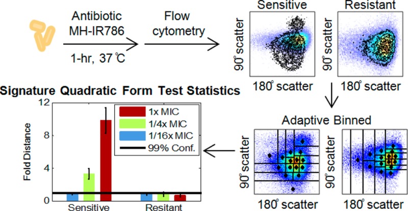
Flow cytometry holds promise to accelerate antibiotic susceptibility determinations; however, without robust multidimensional statistical analysis, general discrimination criteria have remained elusive. In this study, a new statistical method, probability binning signature quadratic form (PB-sQF), was developed and applied to analyze flow cytometric data of bacterial responses to antibiotic exposure. Both sensitive lab strains (Escherichia coli and Pseudomonas aeruginosa) and a multidrug resistant, clinically isolated strain (E. coli) were incubated with the bacteria-targeted dye, maltohexaose-conjugated IR786, and each of many bactericidal or bacteriostatic antibiotics to identify changes induced around corresponding minimum inhibition concentrations (MIC). The antibiotic-induced damages were monitored by flow cytometry after 1-h incubation through forward scatter, side scatter, and fluorescence channels. The 3-dimensional differences between the flow cytometric data of the no-antibiotic treated bacteria and the antibiotic-treated bacteria were characterized by PB-sQF into a 1-dimensional linear distance. A 99% confidence level was established by statistical bootstrapping for each antibiotic-bacteria pair. For the susceptible E. coli strain, statistically significant increments from this 99% confidence level were observed from 1/16x MIC to 1x MIC for all the antibiotics. The same increments were recorded for P. aeruginosa, which has been reported to cause difficulty in flow-based viability tests. For the multidrug resistant E. coli, significant distances from control samples were observed only when an effective antibiotic treatment was utilized. Our results suggest that a rapid and robust antimicrobial susceptibility test (AST) can be constructed by statistically characterizing the differences between sample and control flow cytometric populations, even in a label-free scheme with scattered light alone. These distances vs paired controls coupled with rigorous statistical confidence limits offer a new path toward investigating initial biological responses, screening for drugs, and shortening time to result in antimicrobial sensitivity testing.

The accelerating emergence of multidrug-resistant bacteria and difficulty in rapidly identifying appropriate treatment options are major threats to global public health.¹⁻⁴ The ability of bacteria to rapidly counter newly available antibiotics within only a few years of clinical introduction has also produced “super-bug” infections that are essentially untreatable. Such rapid acquisition of resistance has also decreased both incentives and options for new antibiotic development, with only two new antibiotics having been approved since 2008.^3,5 With 30% of hospital deaths attributable to sepsis, bacterial infections of the blood have become the 10th leading cause of hospital deaths in the US.^6,7 Although rapidly tailored treatment to each individual patient can have a major impact on positive outcome,⁸ currently, nearly 30% of patients receive inappropriate antimicrobial therapy. Such nonideal treatment leads to 2-fold higher mortality rates than when correctly treated⁹ and also contributes to the increase in multidrug-resistance resulting from sublethal antibiotic exposure.^10,11 While rapid initiation of appropriate treatment is crucial to positive patient outcome, only combined knowledge of the pathogen identity and its antibiotic sensitivity profile comprise actionable treatment information. Recent advances that employ mass spectrometry and genetic tests¹²⁻¹⁶ enable identification of an infectious agent within a few hours after positive blood culture. However, conventional antibiotic sensitivity tests (ASTs) typically require overnight subculturing, followed by an 18 to 24 h AST, resulting in a 42–48 h post blood culture delay in susceptibility data. Thus, improving AST time-to-result would have positive patient and public health outcomes.

In many ways resulting from the inability to selectively target bacteria in human specimens, ASTs typically rely on the lengthy process of monitoring growth inhibition of pure cultures under antibiotic challenge. Yet, much smaller antibiotic-induced changes in bacterial cells are likely present long before growth inhibition is detected. To amplify such potentially small changes present at shorter exposure times, large numbers coupled with new multidimensional statistical metrics are needed. Commonly applied in research laboratories for viability testing,^17,18 flow cytometry rapidly measures multichannel fluorescence and scatter from each cell within a large population, yielding large, multidimensional histograms ripe for quantitative statistical analysis. Previously described cytometry-based ASTs mostly rely on interpreting qualitative differences in live and dead cell populations using high-background fluorescent membrane integrity/potential sensors.¹⁹⁻²⁸ Detection of label-free scattered light changes and intracellular reactive oxygen species (ROS) generation in response to antibiotic exposure have also been reported.²⁹⁻³² While advances continue to be made in instrumentation and miniaturization for analyzing bacterial samples,³³⁻³⁷ high background, very large statistical variability, and insufficient changes from controls make many cytometry-based bacteria/antibiotic combinations appear unquantifiable.^23,25,38 Thus, even with a large number of observations probing antibiotic-induced changes within a given cell population, flow cytometic ASTs fail from the lack of accurate statistical metrics to quantify multidimensional changes relative to controls.

Ideally, the dissimilarity between 2 distributions (sample vs control) is quantified by various test statistics, yielding “distances” between measured distributions. One-dimensional test statistics are either too sensitive to provide meaningful analysis^39,40 or required a large number of events⁴⁰ and are usually not rigorously extensible to multidimensional data. Adaptive binning overcomes the data set size and multidimensional extensibility issues to focus analysis on the most informative regions of the data;^41,42 however, sample comparison is control-specific in probability binned chi-square (PB-χ²) tests, making the test result unsuitable as a true (linear) metric for directly comparing multiple samples. As a consequence, it is difficult to adjust statistical tests for biological variability. Various multidimensional distance metrics are known, but necessary computational resources tend to scale with the number of bins raised to some large power. Scaling quadratically with the number of bins, quadratic form (QF) distance statistics directly addresses the metric issue, providing a linear distance between any two multidimensional data sets,⁴³ but its reliance on fixed bin sizes can limit its extension to multidimensional cytometry data sets. Instead of comparing occurrences in fixed bins, adaptively binned or “signature” QF (sQF) has been developed for image analysis to directly compare signatures, or the most important features, within images.^44,45 We have combined the adaptive probability binning with the signature QF distances to create a linear statistical metric that more readily scales to multiple dimensions. Combining the best attributes of PB-χ² and sQF 2D image analysis, our PB-sQF approach focuses binning on the high-density regions of the data, better facilitating true distance comparisons among multidimensional data sets.

Utilizing the fact that bacterial uptake systems have broad substrate specificities, Ning et al.⁴⁶ recently reported that bacteria can be selectively targeted through the maltodextrin uptake pathway. In contrast to other technologies, fluorescently labeled maltohexaose is selectively taken up by bacteria to reach mM intracellular concentrations, without detectable mammalian cell uptake, both in vitro and in vivo.⁴⁶ Such selective labeling offers a way to potentially identify bacterial populations prior to time-consuming subculturing and growth. Thus, using both label-free scattered light and selective bacterial fluorescent labeling through the bacteria-selective maltodextrin metabolic pathway, we have developed a framework for rapidly determining bacterial antibiotic sensitivities. By specifically labeling bacteria with maltohexaose-conjugated IR786 (MH-IR786), coupled with our development of an adaptively binned multidimensional statistical metric combining the best attributes of PB-χ² adaptive binning^41,42 and sQF image analysis,^44,45 we develop a rapid, quantitative flow cytometric approach to determine antibiotic sensitivities even in difficult-to-determine antibiotic-bacterium combinations.

Experimental Section

Media and Antibiotics

E. coli ATCC33456 and P. aeruginosa ATCC27853 were grown in Luria–Bertani (LB) medium (Sigma-Aldrich, St. Louis, MO). The resistant E. coli clinical isolate, Mu14S, was obtained from the Georgia emerging infection program (GEIP). All antibiotics were obtained from Sigma or as otherwise indicated. The E. coli (ATCC 33456) MICs for each antibiotic were measured to be 32 μg/mL penicillin G, 0.125 μg/mL norfloxacin (Enzo Life Science, Farmingdale, NY), 0.016 μg/mL ciprofloxacin, 8 μg/mL kanamycin (Fisher Scientific, Waltham, MA), 1 μg/mL tetracycline, 150 μg/mL erythromycin, 8 μg/mL azythromycin (TCI America, Portland, Oregon), and 2 μg/mL gentamicin (Life Technologies, Carlsbad, CA). The MICs for the E. coli Mu14S strain were as follows: 4 μg/mL gentamicin, > 5000 μg/mL penicillin G, > 8 μg/mL tetracycline. The P. aeruginosa (ATCC 27853) MICs were as follows: 1024 μg/mL kanamycin, 512 μg/mL ampicillin, 16 μg/mL tetracycline, and 2 μg/mL norfloxacin.

Bacterial Strains and Culture

Bacteria were cultured overnight in an incubator shaker (MaxQ 4000, Thermo Fisher Scientific, Waltham, MA) in growth medium at 37 °C and 225 rpm. Bacteria were then reinoculated in 12 mL of fresh LB medium in 50 mL tubes and incubated from ∼0.05 optical density, judging from extinction at 600 nm, to the mid log phase. For antibiotic susceptibility measured by MH-IR786, bacteria in 1 mL of media were collected by centrifugation (Centrifuge 5417R, Eppendorf) at 13,400 rpm for 3 min and transferred into 12-well plates (Costar, New York, NY). Antibiotics at the specified concentrations and 20 μL of MH-IR786 to achieve a final concentration 900 nM were added simultaneously. The 12-well plates were incubated at 37 °C for 1 h (Isotemp standard incubator, Fisher Scientific, Waltham, MA). Bacteria were again collected by centrifugation and washed 3 times with phosphate buffered saline (PBS) (Life Technologies, Carlsbad, CA) and resuspended in 1 mL of PBS. The bacteria samples were maintained on ice until flow cytometry and imaging.

Flow Cytometry

Bacteria samples were analyzed by a BD LSR II flow cytometer (Becton Dickinson, Franklin Lake, NY) equipped with a 14 mW, 488 nm solid-state coherent sapphire laser for the scatter signal and a HeNe Laser (18 mW @ 633 nm) for IR786 detection. Samples were gated by forward and side scatter, while a 750–810 nm bandpass filter was used to collect the IR786 fluorescence signal. Data were collected with FACSDiVa provided by BD. Further data analysis and display were carried out with Matlab 2013b (Math Works). For each data set, 100,000 bacterial detection events were collected.

PB-sQF Test Statistics

The statistical tests were performed in Matlab 2013b on an AMD phenom II X4 820 (2.80 GHz) machine, equipped with 4 GB DDR3 RAM running MS Windows 7. Probability binning codes were written to be equivalent to those described in published studies.^41,42 In brief, probability binning bins the data into approximately equal counts/bin by varying bin width. Binning is performed by calculating the variance of each dimension, identifying the highest variance dimension, and dividing data at the median into two new bins for the high variance dimension. Data on the median are randomly assigned to daughter bins. This process enabled all the bins to have similar counts. Both the control and sample were binned in the same manner, and the centroids and weights of each bin were calculated. The test statistics were then calculated as described in sQF applications using these described centroids and weights.^44,45

The weight vector, which represents the probability of data points falling into each bin (number of events in each bin divided by the total number of events), includes weights from the control and the sample as shown below:

The subscripts indicate whether the weights were taken from the control (C) or the sample (S), and the superscripts indicate the bin for which the weights are calculated. The total number of bins is denoted by N. The negative sign in front of the sample weights was used to make sure that subtraction would be carried out between the control and sample data in the later steps to measure the differences between the two. Although the terminology adopted here is that utilized in sQF image analysis,^44,45 these weights simply represent the different normalized histogram bin counts of control and sample data sets used in standard quadratic form analyses.⁴³

The centroid vector is calculated from the geometric median (or “Geometric quantile”, see below) to represent multidimensional median:

The subscripts and superscripts are the same as in the weight vector. The centroids are then used to calculate the similarity matrix. We defined the matrix elements at the i^th row and the j^th column, A_ij, in the similarity matrix, A, as

The second term is the dissimilarity matrix with the numerator denoting the Euclidean distance between centroids i and j. The denominator is the normalized factor with L_max indicating the maximum distance in each dimension. Since we are dealing with the same dynamic range in every dimension, the maximum distance for n dimensions is L_max·√n. When the two centroids are exactly the same, the numerator is 0, meaning no dissimilarity exists. On the other hand, due to the normalization, when the distance between two centroids equals the dynamic range (the largest possible distance between two centroids), the dissimilarity is 1, representing a full dissimilarity. The similarity matrix, which is the logical opposite of the dissimilarity matrix, is 1 minus the dissimilarity as shown above. The diagonal elements of the similarity matrix are always 1, indicating that each centroid is most similar to itself. The test statistics were calculated using the QF matrix operation:

Weight^T is the transpose of the Weight vector. The test statistics of antibiotic-treated data were then normalized by the 99% confidence level of its paired control. In this paper, we calculated the 3-dimentional test with 128 bins.

Confidence Level Estimation

The bootstrap method was used to determine the 99% confidence level. The flow data of the no-antibiotic control and the 1/16x data were treated as two mother distributions, and 70 daughter distributions with the corresponding sample size, ranging in bacterial counts from 4*(number of bins) to (8000 + minimum sample size) with step size 400, were subsampled from each mother distribution. These distributions were then binned, and the PB-sQF protocol was followed to calculate the test statistics. For each sample size, test statistics were calculated between all 70 of the no-antibiotic control subdistributions and all 70 of the 1/16x data subdistributions. The distance measurements between all pairs of control-1/16x MIC daughter distributions yield a distribution of test statistics values, resulting from random subsampling from the mother distributions (biological variability). The 99% confidence level of all the test statistics at each sample size can be determined. The distance corresponding to the confidence level decreased as the subsample size increased and can be fit by an equation similar to the standard error of the sample mean: Conf(n) = a0 + a1/√n, where Conf is the 99% confidence level value, n is the sample size, and a0 and a1 are the fitting parameters (Figure S6C). Here, a0 is the unknown confidence level of the population. According to central limit theorem, the test statistics distribution of the subdistributions should approximate a Gaussian distribution at large sample size. Thus, the uncertainty (standard error) in estimating the population’s confidence level should follow a1/√n. The observed confidence level then decreases with the inverse square root of the number of data points. As subsample size increases, the deviations become smaller and the estimation converges to the population confidence level. From the fitting, we can then estimate the 99% confidence level of the mother distribution with a sample size, n = 100,000.

Error Bar Determination

The error bars in the test statistics bar charts combine two different uncertainties. One results from biological variability, while the other arises from the dispersion of data points. Biological variability is estimated by the standard deviation of the normalized test statistics of the triplicate data. Errors from binning account for the uncertainty in accurately determining the centroid position within each bin. Median absolute deviation (MAD) is used to measure the dispersion of each bin since it is more robust toward outliers compared to standard deviation. The MAD is calculated as follows:

That is, it is the median of the absolute distance between each data point, X_i, and the centroid of each bin.^53,54 The MAD can then be used to estimate the standard deviation by

where φ^–1 is the inverse of the cumulative distribution function or the quantile function.⁵⁴ As a result, the standard deviation estimated from MAD is the MAD divided by the 75% quantile, which was determined from the geometric quantile. The uncertainty from each bin, σ_perbin^MAD, was then propagated to yield the final binning uncertainty for replica “i”, σ_i.

The binning uncertainty from each replica was then pooled together to estimate the variance of the unknown population, where all triplicate data were presumably sampling from this same unknown population

in which k = 3, since we have triplicate data. n_i is the sample size of each replica, which will be close to 100,000 data points (n_i will be exactly 100,000 if no gate is applied before analysis).

The errors from triplicate data and from the binning process were then propagated together to yield the final uncertainty.

The error bars in the bar charts are one standard deviation above and below the test statistic value.

Geometric Quantiles

Geometric quantiles are applied first in determining the centroid of each bin and second in estimating the error from binning. The whole process uses the quasi-Newton method to solve an unconstrained minimization problem. The target function that we minimize here, as described by Chaudhuri⁵⁵ is

in which n is the number of data points in each bin; X⃗_i is the data point; and Q⃗^(m) is the quantile of the m_th iteration; u = 2α – 1, where α is the fractional quantile. For example, α = 0.5 if we are calculating median (50% quantile). The target function then reduces to f(Q⃗^(m) = ∑_i=1ⁿ{|X⃗_i – Q⃗^(m)|}). The median is the Q that minimizes the sum of distances between each data point to the median. When u is nonzero, the second term in the target function takes the deviation from the median into account. Our initial guess, Q⃗⁽⁰⁾, is the 1-D quantile in each dimension. Q⃗⁽¹⁾ is estimated using the following equations:

in which s⃗^(m) is the increment determined by the first- and second-order derivative of the target function at the current iteration. For each step, we need to examine whether f(Q⃗^(m+1)) < f(Q⃗^(m)). If not, we need to choose a better Q⃗^(m+1).⁵⁶

The iteration stops when either (1) the iteration has been carried out 50 times, with incremental change, δ ≤ s⃗^(m), or (2) the relative gradient in Q is smaller than the stopping criteria we set. The relative gradient is

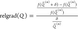In this work, the iteration was stopped when relgrad(Q) is smaller than 10^–4.

Results

Sample Preparation and Data Collection

Bacterial strains were incubated with 900 nM MH-IR786 and antibiotics at their respective 1x, 1/4x, and 1/16x MIC concentrations that were first determined by standard microbroth dilution assays (Table 1). After 1-h incubation, bacteria were pelleted, washed 3 times, and resuspended in PBS for cytometry analyses. Three major bactericidal antibiotics classes, β-lactams (penicillin G and ampicillin), quinolones (ciprofloxacin and norfloxacin), and aminoglycosides (kanamycin and gentamicin) as well as bacteriostatic antibiotics (tetracycline, erythromycin, and azithromycin) that target various biological processes were examined with a total processing time of <4 h.

Table 1. MIC (μg/mL) for Each Antibiotic/Bacteria Combination.

	Pen G	Amp	Nor	Cip	Kan	Tet	Ery	Azi	Gen
E. coli ATCC 33456	32		0.125	0.016	8	1	150	8	2
E. coli Mu14S	>5000					>8			4
P. aeruginosa ATCC 27853		512	2		1024	16

Fluorescence and scatter signals upon antibiotic challenge were monitored by flow cytometry. IR786 fluorescence, forward-scattered and side-scattered light were all collected for each of 100,000 measured bacterial cells per run, yielding 3-D histograms for each antibiotic concentration. All experiments were performed in triplicate and compared to appropriate paired no-antibiotic controls. Using the entire data set as the initial “bin”, data were adaptively binned by splitting the data in each bin at the median of the dimension of highest variance. Each daughter bin was then similarly split at the median of its highest variance dimension until the desired number of bins is achieved. Details on this probability-binning algorithm are given in the Experimental Section. Test results were calculated between each antibiotic data set and its paired control, the antibiotic-free, MH-IR786-labeled bacterial data. A 99% confidence level was determined by bootstrapping and was unique for each no-antibiotic control-1/16x MIC sample pair (details in the Experimental Section). Test results for each bacterium/antibiotic combination were normalized to its own 99% confidence distance, directly reporting on differences between antibiotic-treated samples vs no-antibiotic paired controls. These individually normalized test results, or “fold distances” from each individual paired control, are then directly compared among all antibiotic exposure data. Fold distances from paired controls are plotted as averages of triplicates with standard deviations representing biological variability and intrabin data dispersion (see the Experimental Section for more detail). Test results were considered statistically distinguishable beyond error bars, allowing identification of antibiotic-induced effects. Normalizing test results by the 99% confidence level of each paired control, removes machine-to-machine and day-to-day variations, facilitating direct comparisons.

Antibiotic-Induced Changes in Susceptible E. coli

Data of E. coli (ATCC 33456) treated for 1-h with penicillin G, tetracycline, and kanamycin are shown in Figure 1 (Complete flow cytometry histograms with additional antibiotics can be found in Figures S1 and S2). Upon penicillin G treatments at near MIC concentrations, both scatter and fluorescence signals significantly shift (Figure 1A and 1D). Tetracycline, a bacteriostatic antibiotic targeting the 30S subunit of the bacterial ribosome, however, primarily altered only scatter signals relative to the no-antibiotic control (Figure 1B vs 1E). Conversely, kanamycin, another drug targeting the 30S ribosome, only induced very minor scatter changes, consistent with prior reports with aminoglycoside antibiotics,³⁰ but the fluorescence signal from MH-IR786 clearly increases upon 1x MIC exposure (Figure 1C and 1F). Although MH-mediated dye uptake has been shown to occur via the LamB transporter in E. coli,⁴⁶ it is clear that MH-dye concentration further increases upon near-MIC challenge with certain antibiotics. This provides additional distance-based discrimination of antibiotic-challenged bacteria vs paired controls. Thus, multidimensional statistical metrics that combine both scatter and fluorescence are needed for generalizable, quantitative differentiation of population changes relative to paired controls.

Figure 1.

Antibiotic-induced signal changes. All data were collected in the presence of MH-IR786. (A to C) Scatter signal changes for different antibiotics. The pseudocolor plots are the no-antibiotic data. The overlay contour plots were data of the 1x MIC treatment. (A) Penicillin G, (B) tetracycline, (C) kanamycin. (D to F) Fluorescence signal changes from 1/16x MIC to 1x MIC and the no-antibiotic control. Gray curve: no antibiotic. Blue curve: 1/16x MIC. Green curve: 1/4x MIC. Red curve: 1x MIC. (D) Penicillin G, (E) tetracycline, (F) kanamycin. (G) The PB-sQF results of the 3D data. Black line: 99% confidence level from the test statistics between no-antibiotic control and 1/16x MIC data. All the data were normalized by the confidence level. Blue bar: 1/16x MIC. Green bar: 1/4x MIC. Red bar: 1x MIC.

Incorporating uncertainties arising from both biological variability and intrabin data dispersion into PB-sQF (see the Experimental Section), all test results (Figure 1G) demonstrate statistically significant distances of the 1x MIC data from that of the 1/16x MIC data, that is, beyond the 99% confidence level. Clear trends and transitions occur for all antibiotic/bacteria combinations with increasing antibiotic concentrations. The tested antibiotics target a wide range of processes (DNA replication, protein synthesis, or cell wall synthesis), yet, when using our multidimensional statistical metric that reduces all differences to a single linear distance from its paired control, all classes of antibiotics showed discernible, statistically significant changes in flow cytometry signals. Underpinning the flow cytometry/PB-sQF results, phase-contrast images of E. coli show clear morphology changes resulting from antibiotic treatment (Figure S3). Note that the 99% confidence level, which was determined by the bootstrap method of calculating the test statistics between the subsampling daughter distributions of the no-antibiotic control and the 1/16x MIC data at small sample size, accurately estimates the 99% confidence level distance between the two mother distributions. Thus, distances among all individually binned multidimensional histograms are reduced to single linear distances relative to paired controls using our PB-sQF distance metrics, enabling antibiotic sensitivities to be determined after only 1-h exposures in comparison to overnight incubation in standard ASTs.

Cytometric Susceptibility Analysis of a Resistant E. coli Clinical Isolate

To evaluate the antibiotic-induced changes in resistant strains, we examined a multidrug resistant, clinically isolated E. coli, Mu14S. Mu14S was susceptible to gentamicin but was highly resistant to all other tested antibiotics (Table 1). We examined both the laboratory strain (ATCC 33456) and Mu14S with penicillin G, tetracycline, and gentamicin in parallel. Consistent with the data shown in Figure 1, incubation with penicillin G at 1x MIC of ATCC33456 strain clearly shifts its scatter and fluorescence distributions (Figures 2A and S4) while not affecting those of the resistant clinical strain Mu14S (Figures 2D and S4). The 3D data (forward scatter, side scatter, and fluorescence) from both strains were quantified with PB-sQF (Figure 2G). Analysis confirmed that penicillin G was effective toward ATCC with both 1/4x and 1x MIC extending above the 1/16x–no-antibiotic, 99% confidence level, while all Mu14S results were below the 99% confidence level, indicating that PB-sQF registers no significant changes at these concentrations. On the other hand, while tetracycline induced scatter changes in ATCC33456 (Figure 2B) without clear fluorescence shifts (Figure S4), neither scatter nor fluorescence signals shifted upon tetracycline exposure in Mu14S strain (Figures 2E and S4). The PB-sQF results confirmed the ATCC33456 sensitivity and Mu14S resistance toward tetracycline (Figure 2H).

Figure 2.

Signal changes induced by antibiotic treatments in E. coli with different susceptibilities. All data were collected in the presence of MH-IR786. (A to F) Scatter signal changes. The pseudocolor plots are the no antibiotic paired control, for each strain. The overlaid contour plots are the 1x MIC antibiotic concentration scatter data. (A to C) The lab strain E. coli (ATCC 33456). (D to F) The multidrug clinical strain E. coli (Mu14S). (G to I) PB-sQF 3D test results. First column (A, D, and G) penicillin G; second column (B, E, and H) tetracycline; third column (C, F, and I) gentamicin. Penicillin G and tetracycline were examined at the 1x, 1/4x, and 1/16x of MIC of ATCC (32 and 1 μg/mL, respectively). Gentamicin was applied at the MIC of Mu14S (4 μg/mL). FSC: forward scatter. SSC: side scatter. (Corresponding fluorescence data can be found in the Supporting Information).

The MICs for ATCC33456 and Mu14S of gentamicin are 2 μg/mL and 4 μg/mL, respectively. Both strains were incubated with gentamicin at the MIC of Mu14S. Gentamicin induced very little scatter and fluorescence shifts in either strain (Figures 2C, 2F, S4). However, our improved statistical metrics enable accurate quantification of these small differences (Figure 2I). Even with triplicate and centroid uncertainties, the test results registered significant changes from 1/4 μg/mL to 4 μg/mL for both strains, confirming the microbiological report, but with only 1-h exposure.

P. aeruginosa Characterized by Flow Cytometry and PB-sQF

Previous studies have shown that P. aeruginosa strains are particularly difficult test cases with most antibiotics in which bacterial viability tests routinely fail.²⁵ For P. aeruginosa, this was explained by its outer membrane interaction with the dye propidium iodide (PI), yielding too high a background. Thus, we applied our 3D PB-sQF to P. aeruginosa using four different antibiotics. Using PB-sQF, P. aeruginosa exhibits readily distinguished sample-control distances analogous to those in E. coli, upon near MIC exposure to the same antibiotics (Figure 3 and Figure S5). In the fluorescence data (Figure 3B and Figure S5), it is clear that a single threshold is difficult to establish without any false positive or false negative counts since the control curve significantly overlaps the antibiotic-treated distributions. By directly comparing the whole data set, PB-sQF removes the need for artificial thresholds, enabling quantitative comparisons.

Figure 3.

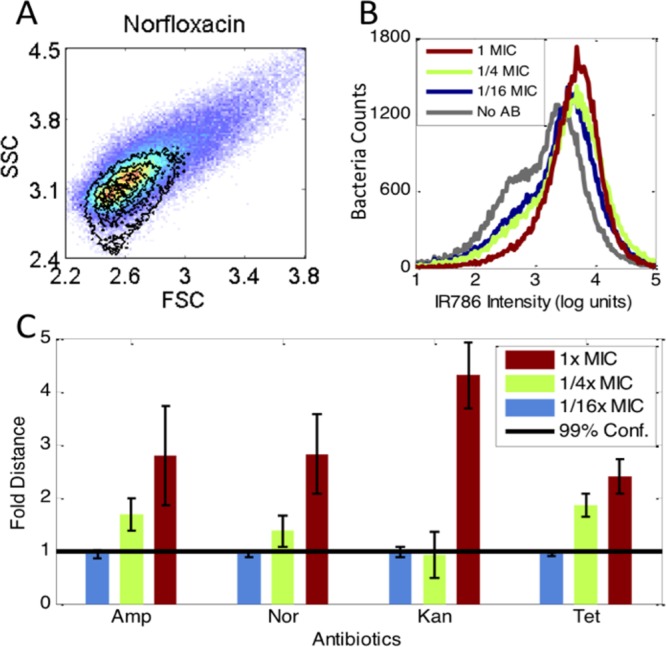
PB-sQF registered antibiotic-induced signal changes in P. aeruginosa. (A) Scatter signal changes by norfloxacin. The pseudocolor plots are the no antibiotic control. The contour plots lay above were the 1x MIC scatter data. (B) Norfloxacin-induced MH-IR786 fluorescence signal changes. (C) The 3D PB-sQF test results for norfloxacin and other antibiotics-induced signal changes.

Discussion

Historically, specific bacteria/antibiotic combinations have been especially difficult to assay with flow cytometric scatter or viability testing. For example, ciprofloxacin with E. coli,²³ tetracycline, and norfloxacin with several bacterial species and most antibiotics with P. aeruginosa are particularly difficult test cases in which bacterial viability tests routinely fail.²⁵ Using our 3D PB-sQF, we have demonstrated not only the difficult-to-determine E. coli sensitivity to either ciprofloxacin, tetracycline, or norfloxacin (Figure 1) but also that P. aeruginosa exhibits readily distinguished sample-control distances similar to those in E. coli, upon near MIC exposure to antibiotics.

Due to the large possible signal shifts, fluorescence-based viability tests are typically preferred over scattered light signals in flow cytometry. Frequently, only weakly quantitative distribution averages and standard deviations or intensity ratios are used to qualitatively discern differences among samples, instead of using appropriate multidimensional statistical tests with paired controls.^{22,23,25,28,29,47,48} This lack of statistical rigor has prevented antibiotic susceptibility of many bacteria/antibiotic combinations from being determinable with rapid cytometric methods. The quantitative PB-χ² methods^41,42 from which we have adapted our binning methods have been a significant advance in analysis. However, sample differences do not yield linear distances from calculated test statistics, suggesting that PB-χ² is not a statistical metric and preventing all samples from being directly compared on the same distance axis. This was confirmed in our studies as we increased the differences between the data and sample, a linear increase was not obtained in the test value (Figure S6A). Thus, test results between subdistributions could not be directly aligned on the same scale, clouding direct comparisons to paired controls. Although for data with larger PB-χ² test statistics vs the same control with the same binning pattern, greater test statistic differences indicate smaller similarity with the control. However, not knowing the response curve, it precludes knowing how different the two data sets actually are. Further, since all the data all must be binned according to the control binning pattern, the response curves might possess different curvature when different controls are used. Confounding comparisons among data from different days or machines, this control-dependent property might also contribute to error in test statistics when triplicate (or more) data with their own paired-control are considered. Nonetheless, our bootstrap method can also be applied to PB-χ², and a 99% confidence level can be determined from fitting (Figure S6B). This 99% confidence level can be used as a threshold, and a similar bar chart regarding antibiotic susceptibility can be created. Although the fold distance is less meaningful here, a similar AST can still be built. PB-sQF directly circumvents these problems by combining the linear aspect of QF statistics with probability binning to better interpret the flow cytometry data, each with its own optimal binning.

Flow cytometry data are most typically qualitatively analyzed by setting artificial thresholds using either membrane potential or membrane permeability dyes.^25,28,47 Usually applicable only to 1-D data, statistical methods employed in flow scale quadratically or faster with the number of bins and either subject to specific binning pattern and/or cannot be scaled to multidimensional data sets.^39,40 PB-sQF scales quadratically with the number of bins, which are concentrated around the data signatures due to the adaptive binning process. The linear distance among bin centroids and comparisons to paired controls removes machine-specific variabilities, while biological variations can be quantitatively incorporated. In PB-sQF, a statistical threshold is easily established by bootstrapping without any assumption of the data distributions. Test results can be normalized by this statistical threshold so data from different machines or collected on different days can be compared directly in a “fold distance” fashion. PB-sQF is a new, robust statistical metric exhibiting more advantageous scaling to multiple dimensions than even QF, as it requires fewer bins in each dimension–naturally adapting to where the data points cluster (the signatures). Each data set is adaptively binned, and the distance between signatures or binning patterns is directly calculated and can be directly compared for each multidimensional histogram, thereby enabling direct comparisons of sample with paired negative controls for excellent discrimination of differences in response to antibiotic concentrations.

As maltohexaose conjugates are believed to be incorporated into bacteria via active uptake processes,^46,49 shifts in MH-targeted fluorescence signals likely indicate changes in bacterial physiological status. Forward and side scatter, however, provide label-free measurements that largely reflect cell size/morphology and internal cellular structure/granularity, respectively.⁵⁰ Indeed, images of bacteria at near-MIC antibiotic levels are often elongated relative to those without antibiotic present (Figure S3). Also, antibiotic-induced filamentation has been observed to result from exposure to β-lactam,^21,51 quinoline,^21,29 and bacteriostatic⁵² antibiotics. Although it is not clear how these antibiotics, with different primary targets, uniformly induce changes in morphology and/or physiology, their changes in flow data from no-antibiotic controls appear to be generally correlated with antibiotic sensitivity levels.

Conclusion

By analyzing bacterial flow cytometry data after only 1-h incubation, the quantitative statistical metric, PB-sQF identifies the data signatures and compares them by reducing multidimensional differences to a linear distance between antibiotic-treated data and paired no-antibiotic controls. With rigorous uncertainties incorporated, subtle, but biologically relevant, antibiotic-induced changes become directly quantifiable, even as these antibiotics target widely varying biological pathways including DNA replication, protein synthesis, or cell wall synthesis.³² Thus, scattered light and bacteria-targeted fluorescence, coupled with new statistical metrics, appear to more generally enable rapid flow cytometry signal changes to gauge antibiotic resistance over a wide range of bacteria/antibiotic combinations. Even very difficult to discern combinations that fail with viability tests are readily distinguished with our statistical measures that are scalable to multiparameter measurements.

With potential to improve patient outcomes through shortening the window during which empiric antibiotic treatment is the only recourse, flow-based antibiotic sensitivity determination suggests a >10-fold reduction in post blood culture time to result (∼42 h to ∼4 h). As antibiotic susceptibilities and resistance proliferation are of great concern, these results suggest a path toward more effective and timely treatment. As time to treatment is a major determinant of positive patient outcome, the strong correlation of sample-control distance in combined scatter and fluorescence shifts with antibiotic sensitivity strongly suggests that general criterion can be established for developing robust flow cytometric based, rapid ASTs.

Supporting Information Available

Additional figures and data on changes in bacterial morphology and fluorescence when challenged with antibiotics and linearity comparisons of PB-χ² vs PB-sQF statistics. This material is available free of charge via the Internet at http://pubs.acs.org.

The authors declare no competing financial interest.

Funding Statement

National Institutes of Health, United States

References

- Arias C. A.; Murray B. E. N. Engl. J. Med. 2009, 360, 439–443. [DOI] [PubMed] [Google Scholar]
- Master R. N.; Deane J.; Opiela C.; Sahm D. F. Ann. N.Y. Acad. Sci. 2013, 1277, 1–7. [DOI] [PubMed] [Google Scholar]
- Boucher H. W.; Talbot G. H.; Benjamin D. K.; Bradley J.; Guidos R. J.; Jones R. N.; Murray B. E.; Bonomo R. A.; Gilbert D.; America f. t. I. D. S. o. Clin. Infect. Dis. 2013, 10.1093/cid/cit152. [DOI] [PMC free article] [PubMed] [Google Scholar]
- Klevens R.; Morrison M. A.; Nadle J.; et al. JAMA 2007, 298, 1763–1771. [DOI] [PubMed] [Google Scholar]
- Boucher H. W.; Talbot G. H.; Bradley J. S.; Edwards J. E.; Gilbert D.; Rice L. B.; Scheld M.; Spellberg B.; Bartlett J. Clin. Infect. Dis. 2009, 48, 1–12. [DOI] [PubMed] [Google Scholar]
- Boucher H. W.; Corey G. R. Clin. Infect. Dis. 2008, 46, S344–S349. [DOI] [PubMed] [Google Scholar]
- Heffner A. C.; Horton J. M.; Marchick M. R.; Jones A. E. Clin. Infect. Dis. 2010, 50, 814–820. [DOI] [PMC free article] [PubMed] [Google Scholar]
- Doern G. V.; Vautour R.; Gaudet M.; Levy B. J. Clin. Microbiol. 1994, 32, 1757–1762. [DOI] [PMC free article] [PubMed] [Google Scholar]
- Ibrahim E. H.; Sherman G.; Ward S.; Fraser V. J.; Kollef M. H. Chest 2000, 118, 146–155. [DOI] [PubMed] [Google Scholar]
- Chen K.; Sun G. W.; Chua K. L.; Gan Y.-H. Antimicrob. Agents Chemother. 2005, 49, 1002–1009. [DOI] [PMC free article] [PubMed] [Google Scholar]
- Kohanski M. A.; DePristo M. A.; Collins J. J. Mol. Cell 2010, 37, 311–320. [DOI] [PMC free article] [PubMed] [Google Scholar]
- Christner M.; Rohde H.; Wolters M.; Sobottka I.; Wegscheider K.; Aepfelbacher M. J. Clin. Microbiol. 2010, 48, 1584–1591. [DOI] [PMC free article] [PubMed] [Google Scholar]
- Fothergill A.; Kasinathan V.; Hyman J.; Walsh J.; Drake T.; Wang Y. F. J. Clin. Microbiol. 2013, 51, 805–809. [DOI] [PMC free article] [PubMed] [Google Scholar]
- Peters R. P. H.; Savelkoul P. H. M.; Simoons-Smit A. M.; Danner S. A.; Vandenbroucke-Grauls C. M. J. E.; van Agtmael M. A. J. Clin. Microbiol. 2006, 44, 119–123. [DOI] [PMC free article] [PubMed] [Google Scholar]
- Barken K. B.; Haagensen J. A. J.; Tolker-Nielsen T. Clin. Chim. Acta 2007, 384, 1–11. [DOI] [PubMed] [Google Scholar]
- Barczak A. K.; Gomez J. E.; Kaufmann B. B.; Hinson E. R.; Cosimi L.; Borowsky M. L.; Onderdonk A. B.; Stanley S. A.; Kaur D.; Bryant K. F.; Knipe D. M.; Sloutsky A.; Hung D. T. Proc. Natl. Acad. Sci. U. S. A. 2012, 109, 6217–6222. [DOI] [PMC free article] [PubMed] [Google Scholar]
- Berney M.; Hammes F.; Bosshard F.; Weilenmann H.-U.; Egli T. Appl. Environ. Microbiol. 2007, 73, 3283–3290. [DOI] [PMC free article] [PubMed] [Google Scholar]
- Breeuwer P.; Abee T. Int. J. Food Microbiol. 2000, 55, 193–200. [DOI] [PubMed] [Google Scholar]
- Mason D. J.; Allman R.; Stark J. M.; Lloyd D. J. Microsc. 1994, 176, 8–16. [DOI] [PubMed] [Google Scholar]
- Walberg M.; Gaustad P.; Steen H. B. J. Antimicrob. Chemother. 1996, 37, 1063–1075. [DOI] [PubMed] [Google Scholar]
- Walberg M.; Gaustad P.; Steen H. B. Cytometry 1997, 27, 169–178. [PubMed] [Google Scholar]
- Suller M. T. E.; Lloyd D. Cytometry 1999, 35, 235–241. [DOI] [PubMed] [Google Scholar]
- Mortimer F. C.; Mason D. J.; Gant V. A. Antimicrob. Agents Chemother. 2000, 44, 676–681. [DOI] [PMC free article] [PubMed] [Google Scholar]
- Walberg M.; Steent H. B. In Methods in Cell Biology; Darzynkiewicz Z., Crissman H. A., Robinson J. P., Eds.; Academic Press: 2001; pp 553–566. [DOI] [PubMed] [Google Scholar]
- Gauthier C.; St-Pierre Y.; Villemur R. J. Med. Microbiol. 2002, 51, 192–200. [DOI] [PubMed] [Google Scholar]
- Assunção P.; Antunes N. T.; Rosales R. S.; Poveda C.; De La Fe C.; Poveda J. B.; Davey H. M. J. Appl. Microbiol. 2007, 102, 1132–1137. [DOI] [PubMed] [Google Scholar]
- Faria-Ramos I.; Espinar M. J.; Rocha R.; Santos-Antunes J.; Rodrigues A. G.; Cantón R.; Pina-Vaz C. Clin. Microbiol. Infect. 2013, 19, E8–E15. [DOI] [PubMed] [Google Scholar]
- Nuding S.; Zabel T. L. J. Bacteriol. Parasitol. 2013, S5, 005. [Google Scholar]
- Wickens H. J.; Pinney R. J.; Mason D. J.; Gant V. A. Antimicrob. Agents Chemother. 2000, 44, 682–687. [DOI] [PMC free article] [PubMed] [Google Scholar]
- Gant V. A.; Warnes G.; Phillips I.; Savidge G. F. J. Med. Microbiol. 1993, 39, 147–154. [DOI] [PubMed] [Google Scholar]
- Kohanski M. A.; Dwyer D. J.; Hayete B.; Lawrence C. A.; Collins J. J. Cell 2007, 130, 797–810. [DOI] [PubMed] [Google Scholar]
- Kohanski M. A.; Dwyer D. J.; Collins J. J. Nat. Rev. Microbiol. 2010, 8, 423–435. [DOI] [PMC free article] [PubMed] [Google Scholar]
- Oakey J.; Applegate R. W.; Arellano E.; Carlo D. D.; Graves S. W.; Toner M. Anal. Chem. 2010, 82, 3862–3867. [DOI] [PMC free article] [PubMed] [Google Scholar]
- Madren S. M.; Hoffman M. D.; Brown P. J. B.; Kysela D. T.; Brun Y. V.; Jacobson S. C. Anal. Chem. 2012, 84, 8571–8578. [DOI] [PMC free article] [PubMed] [Google Scholar]
- Wu L.; Luan T.; Yang X.; Wang S.; Zheng Y.; Huang T.; Zhu S.; Yan X. Anal. Chem. 2013, 86, 907–912. [DOI] [PubMed] [Google Scholar]
- Yang L.; Wu L.; Zhu S.; Long Y.; Hang W.; Yan X. Anal. Chem. 2009, 82, 1109–1116. [DOI] [PubMed] [Google Scholar]
- Butterworth P.; Baltar H. T. M. C. M.; Kratzmeier M.; Goldys E. M. Anal. Chem. 2011, 83, 1443–1447. [DOI] [PubMed] [Google Scholar]
- Shapiro H. M. Cytometry 2001, 43, 223–226. [DOI] [PubMed] [Google Scholar]
- Young I. T. J. Histochem. Cytochem. 1977, 25, 935–941. [DOI] [PubMed] [Google Scholar]
- Cox C.; Reeder J. E.; Robinson R. D.; Suppes S. B.; Wheeless L. L. Cytometry 1988, 9, 291–298. [DOI] [PubMed] [Google Scholar]
- Roederer M.; Treister A.; Moore W.; Herzenberg L. A. Cytometry 2001, 45, 37–46. [DOI] [PubMed] [Google Scholar]
- Roederer M.; Moore W.; Treister A.; Hardy R. R.; Herzenberg L. A. Cytometry 2001, 45, 47–55. [DOI] [PubMed] [Google Scholar]
- Bernas T.; Asem E. K.; Robinson J. P.; Rajwa B. Cytometry, Part A 2008, 73A, 715–726. [DOI] [PubMed] [Google Scholar]
- Beecks C.; Uysal M. S.; Seidl T. In Proceedings of the 17th ACM international conference on Multimedia; ACM: Beijing, China, 2009; pp 697–700. [Google Scholar]
- Beecks C.; Uysal M. S.; Seidl T. In Proceedings of the ACM International Conference on Image and Video Retrieval; ACM: Xi’an, China, 2010; pp 438–445. [Google Scholar]
- Ning X.; Lee S.; Wang Z.; Kim D.; Stubblefield B.; Gilbert E.; Murthy N. Nat. Mater. 2011, 10, 602–607. [DOI] [PMC free article] [PubMed] [Google Scholar]
- Shrestha N. K.; Scalera N. M.; Wilson D. A.; Procop G. W. J. Clin. Microbiol. 2011, 49, 2116–2120. [DOI] [PMC free article] [PubMed] [Google Scholar]
- Suller M. T.; Stark J. M.; Lloyd D. J. Antimicrob. Chemother. 1997, 40, 77–83. [DOI] [PubMed] [Google Scholar]
- Boos W.; Shuman H. Microbiol. Mol. Biol. Rev. 1998, 62, 204–+. [DOI] [PMC free article] [PubMed] [Google Scholar]
- Müller S.; Nebe-von-Caron G. FEMS Microbiol. Rev. 2010, 34, 554–587. [DOI] [PubMed] [Google Scholar]
- Chung H. S.; Yao Z.; Goehring N. W.; Kishony R.; Beckwith J.; Kahne D. Proc. Natl. Acad. Sci. U. S. A. 2009, 106, 21872–21877. [DOI] [PMC free article] [PubMed] [Google Scholar]
- Steel C.; Wan Q.; Xu X.-H. N. Biochemistry 2003, 43, 175–182. [DOI] [PubMed] [Google Scholar]
- Cotta J. G.Zeitschrift für Astronomie und verwandte Wissenschaften; 1816. [Google Scholar]
- Ruppert D.Statistics and Data Analysis for Financial Engineering; Springer: 2010. [Google Scholar]
- Chaudhuri P. J. Am. Stat. Assoc. 1996, 91, 862–872. [Google Scholar]
- Dennis J. E. Jr.; Schnabel R. B.. Numerical methods for unconstrained optimization and nonlinear equations; Society for Industrial and Applied Mathematics: 1996; Vol. 16. [Google Scholar]
Associated Data
This section collects any data citations, data availability statements, or supplementary materials included in this article.