

Abstract
A multivariable analysis is the most popular approach when investigating associations between risk factors and disease. However, efficiency of multivariable analysis highly depends on correlation structure among predictive variables. When the covariates in the model are not independent one another, collinearity/multicollinearity problems arise in the analysis, which leads to biased estimation. This work aims to perform a simulation study with various scenarios of different collinearity structures to investigate the effects of collinearity under various correlation structures amongst predictive and explanatory variables and to compare these results with existing guidelines to decide harmful collinearity. Three correlation scenarios among predictor variables are considered: (1) bivariate collinear structure as the most simple collinearity case, (2) multivariate collinear structure where an explanatory variable is correlated with two other covariates, (3) a more realistic scenario when an independent variable can be expressed by various functions including the other variables.
Keywords: multicollinearity effect, multivariable models, collinearity structure, simulation study
Introduction
Multivariable analysis is a commonly used statistical method in medical research when multiple predictive variables are considered to estimate the association with study measurements. However, efficiency of multivariable analysis highly depends on correlation structure among predictive variables since inference for multivariable analysis assumes that all predictive variables are uncorrelated. When the covariates in the model are not independent from one another, collinearity or multicollinearity problems arise in the analysis, which leads to biased coefficient estimation and a loss of power. Numerous studies in epidemiology, genomics, medicine, marketing and management, and basic sciences have reported the effects and diagnosis of collinearity amongst their study variables (Batterham et al. 1997; Wax 1992; Cavell et al. 1998; Mofenson et al. 1999; Elmstahl et al. 1997; Parkin et al. 2002; Kmita et al. 2002). As literature indicates, collinearity increases the estimate of standard error of regression coefficients, causing wider confidence intervals and increasing the chance to reject the significant test statistic. This leads to imprecise estimates of regression coefficients with wrong signs and an implausible magnitude for some regressors because the effects of these variables are all mixed together. Furthermore, it reveals that small change in the data may lead to large differences in regression coefficients, and causes a loss in power and makes interpretation more difficult since there is a lot of common variation in the variables (Vasu and Elmore 1975; Belsley 1976; Stewart 1987; Dohoo et al., 1996; Tu et al., 2005).
How can we assess whether or not collinearity is truly harmful or problematic in the estimation of multivariable models? The literature provides numerous suggestions including the examination of the correlation matrix of the independent variables, computing the coefficients of determination, of each Xk regressed on the remaining predictor variables including the variance inflation factor (VIF), and measuring condition index (CI) based on the singular value decomposition of the data matrix X. This work aims to investigate the effects of collinearity under various correlation structures amongst predictive and explanatory variables, to compare these results with existing guidelines to decide harmful collinearity, and to provide a guideline on multivariable modeling. Following a brief review for effects of collinearity and diagnostic tools, we describe how to generate correlated data, and develop a simulation study with various scenarios of different collinearity structures. We then demonstrate the proper examination of the effects of those different collinearity situations and compare them. Three correlation scenarios among predictor variables are considered: (1) bivariate collinear structure as the most simple collinearity case: only two correlated variables among independent variables, (2) multivariate collinear structure where an explanatory variable is correlated with two other covariates, (3) a more realistic scenario when an independent variable can be expressed by various functions including the other variables.
Effects of Collinearity and Diagnostic Tools
Collinearity or multicollinearity causes redundant information, which means that what a regressor explains about the response is overlapped by what another regressor or a set of other regressors explain. Hair et al. (1998) noted that as multicollinearity increases, it is more difficult to ascertain the effect of any single variable produce biased estimates of coefficients for regressors because the variables have more interrelationships. The effect of collinearity can be investigated with the formula for the variance-covariance matrix of the estimated coefficients.
The variance-covariance matrix for the vector of coefficients, β, are given by
| (1) |
where X is the design matrix and σ2 is the error variance, which is estimated by the sample variance s2. Next we define as the coefficient of determination for a regression with Xk as the dependent variable and the other Xj′s, j ≠ k, as predictor variables. The variance of a specific coefficient βk is given by
| (2) |
where β̂k is the kth entry in β̂; Xik is the entry in the ith row, kth column of X; X̄k is the mean of the kth column (Fox et al. 1992). If the multicollinearity between a kth independent variable Xk and one or more other independent variables increases, Rk becomes larger since it demonstrates the linear relationship between Xk and other variables. The equation (2) indicates that a larger Rk increases the variance of the estimate of the kth regression coefficient, β̂k. The estimated standard deviation of least square estimated regression coefficients, s(β̂k), will increase as the degree of multicollinearity becomes higher. Therefore, larger values of s(β̂k) will also affect the value of a t-test. The test statistic, β̂k/s(β̂k), becomes smaller when the value of s(β̂k) is larger. The confidence interval for the regression coefficients, β̂k ± t × s(β̂k), becomes larger as the estimated standard deviation becomes larger. As a consequence, collinearity causes increased inaccuracy, and can seriously distort the interpretation of a model. Serious distortion yields elevated risk of both false-positive results (Type I error) and false-negative results (Type II error). Note that if multicollinearity is not perfect, the ordinary least square estimate, β̂, is unbiased, still best linear unbiased estimates (BLUE), and will have the least variance among unbiased linear estimators while its variance will increase due to multicollinearity.
The literature provides numerous suggestions, ranging from simple rules of thumb to complex indices, for diagnosing the presence of substantive collinearity. The variance important factors (VIF) is one of the most widely used rules. The VIF for the predictor variable Xk is given by . VIF indicate the strength of the linear dependencies and how much the variances of each regression coefficients is inflated due to collinearity compared to when the independent variables are not linearly related. Despite no formal rule, it is generally accepted that a VIF value greater than 10 may be harmful. As mostly known, we expect that as the degree of collinearity goes seriously, both the variance of the estimate of the kth regressor coefficient and the VIF become larger.
Effects of Collinearity under various Collinear Conditions
A simulation study is performed to examine the effects of bias due to the degree of collinearity amongst independent variables in multivariable linear regression models. Let X be a matrix of three independent variables: X1, X2, and X3; and, let Σ be a variance-covariance matrix of a vector X. Our purpose is to generate the vector X from multivariate normal distribution with mean zero vector and variance-covariance matrix Σ, where Σ is a symmetric 3 by 3 matrix and a positive definite. We can obtain correlated normal variables X = C ′ Z where Z are standard normal random variables and C is an upper triangular matrix such that C ′ C = Σ for any positive definite matrix Σ. Three different scenarios are considered, which have different correlation structures among the variables. First, we begin with the simplest case which assumes that two variables are correlated with each other among three predictive variables in a multivariable model, but the remaining independent variable does not correlate with both the two correlated independent variables. In this bivariate collinearity scenario, we investigate the effect of bias in estimates of related regressor coefficients due to the variation in the degree of collinearity between the two variables in the model. Second, we extend the first scenario by correcting a variable with two other variables, but maintain that there is no correlation between those two variables. Thus, there exist two correlation coefficients in this case. Third, we consider an independent variable which can be obtained by a mathematical function of the other predictive variables in the model. Four different transformation functions which are frequently found in medical research are used to investigate the effect of bias in regressor’s estimates where indirect correlation exists between a calculated variable and the other covariates. They include: (1) ratio of two variables, (2) interaction of two variables, (3) linear combination of two variables, and (4) quadratic form of a variable.
Case 1: Two Variables Aare Correlated with Each Other
This scenario assumes that two (X1 and X3) are correlated with each other and another covariate (X2) is independent with both X1 and X3. We denote r13 as the correlation coefficient between X1 and X3, and considered escalated levels of correlation between two variables X1 and X3. We increase the r13 from zero to one by increments of 0.05 positively, then decrease from zero to minus one by 0.05 negatively. We then investigated the degree to which the estimates for β1, β2, and β3 are seriously affected in the bias magnitude according to different levels of correlation. Our main interest in this scenario is to examine the effect of distortion in estimates of two correlated parameter coefficients, β1 and β3. Table 1 shows the point estimates of three regression, β1, β2, and β3 for covariates X1, X2, and X3 due to the variation of degrees in the correlation coefficients “r13” between zero and plus/minus one. As expected, the estimate of the regression coefficient for a variable X12 is almost unchanged regardless of the variation of the correlation coefficient between X1 and X3 but the estimates of the regressor coefficients for variables of X1 and X3 vary over the different level of correlation coefficient, r13. Both estimates of β1 and β3 have very similar variation of effects in magnitude for both positive and negative correlation structures. The estimates vary smoothly until the correlation reach to 90% positively or to 90% negatively, but vary quite sharply after 90% of positive correlation and 90% of negative correlation. The estimate of β1 is 1.2275 when it is uncorrelated, but show a bias almost twice as great at r13=0.70 (β1 = 2.4780), and increases dramatically when r13 is greater than 0.90. The estimates are 3.8603, 5.1064, and 29.7068 when r13=0.90, 0.95 and 0.99 respectively. The estimate of β3 is similarly biased to the estimate of β1. It also showed a dramatic increase dramatically when r13 is greater than 0.90, and reaches 28.50675 at r13=1.0. Therefore, we see the estimates of β1 and β3 are biased similarly for both covariates. Figure 1 shows the trajectories of the variation of the estimates of three coefficients, β1, β2 and β3, when the correlation coefficient between X1 and X3 varies from zero to one and minus one by a difference of 5%.
Table 1.
Point Estimation of Regressor coefficients for X1, X2, and X3 from Correlated Data Sets Which Had Been Randomly Generated According to Different Correlation Condition between X1 and X3
| True correlation coefficient between X1 and X3 | Parameter estimates of |
True correlation coefficient between X1 and X3 | Parameter estimates of |
||||
|---|---|---|---|---|---|---|---|
| X1 | X2 | X3 | X1 | X2 | X3 | ||
|
| |||||||
| 0.00 | 1.22746 | 0.86001 | 1.27453 | 0.00 | 1.22746 | 0.86001 | 1.27453 |
| −0.05 | 1.29254 | 0.86001 | 1.27613 | 0.05 | 1.16493 | 0.86001 | 1.27613 |
| −0.10 | 1.35683 | 0.86001 | 1.28095 | 0.10 | 1.10064 | 0.86001 | 1.28095 |
| −0.15 | 1.42210 | 0.86001 | 1.28912 | 0.15 | 1.03536 | 0.86001 | 1.28912 |
| −0.20 | 1.48890 | 0.86001 | 1.30082 | 0.20 | 0.96857 | 0.86001 | 1.30082 |
| −0.25 | 1.55782 | 0.86001 | 1.31633 | 0.25 | 0.89965 | 0.86001 | 1.31633 |
| −0.30 | 1.62955 | 0.86001 | 1.33607 | 0.30 | 0.82791 | 0.86001 | 1.33607 |
| −0.35 | 1.70494 | 0.86001 | 1.36059 | 0.35 | 0.75252 | 0.86001 | 1.36059 |
| −0.40 | 1.78498 | 0.86001 | 1.39063 | 0.40 | 0.67248 | 0.86001 | 1.39063 |
| −0.45 | 1.87097 | 0.86001 | 1.42720 | 0.45 | 0.58649 | 0.86001 | 1.42720 |
| −0.50 | 1.96458 | 0.86001 | 1.47171 | 0.50 | 0.49288 | 0.86001 | 1.47171 |
| −0.55 | 2.06808 | 0.86001 | 1.52609 | 0.55 | 0.38938 | 0.86001 | 1.52609 |
| −0.60 | 2.18463 | 0.86001 | 1.59317 | 0.60 | 0.27283 | 0.86001 | 1.59317 |
| −0.65 | 2.31889 | 0.86001 | 1.67716 | 0.65 | 0.13858 | 0.86001 | 1.67716 |
| −0.70 | 2.47803 | 0.86001 | 1.78470 | 0.70 | −0.02056 | 0.86001 | 1.78470 |
| −0.75 | 2.67392 | 0.86001 | 1.92691 | 0.75 | −0.21645 | 0.86001 | 1.92691 |
| −0.80 | 2.92811 | 0.86001 | 2.12422 | 0.80 | −0.47065 | 0.86001 | 2.12422 |
| −0.85 | 3.28528 | 0.86001 | 2.41947 | 0.85 | −0.82782 | 0.86001 | 2.41947 |
| −0.90 | 3.86032 | 0.86001 | 2.92398 | 0.90 | −1.40285 | 0.86001 | 2.92398 |
| −0.95 | 5.10642 | 0.86001 | 4.08178 | 0.95 | −2.64895 | 0.86001 | 4.08178 |
| −1.00 | 29.70680 | 0.86001 | 28.50657 | 1.00 | −27.24934 | 0.86001 | 28.50657 |
Figure 1.
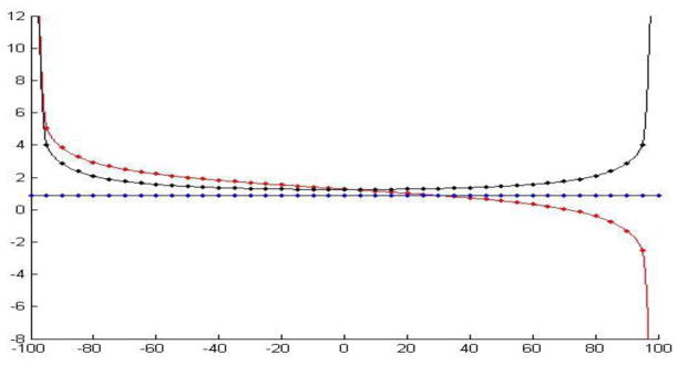
The trajectories of the variation of the estimates of three coefficients, β1, β2 and β3, when the correlation coefficient between X1 and X3 varies from zero to one and minus one by a difference of 5%. X-axis is escalated levels of correlation between two variables X1 and X3 and Y-axis is estimates of three coefficients, β1, β2 and β3. The estimate β1 increases as the correlation coefficient varies from zero to minus one but decreases as the correlation coefficient varies from zero to one goes while the estimate β3 increases as the correlation coefficient varies from zero to one or minus one. The estimate β2 is almost constant regardless of the variation of the correlation coefficient between X1 and X3. (Red line for β1, blue line for β2, and black line for β3).
The 95% confidence intervals for those three coefficients were examined to see how much they were affected by the degree of collinearity. Table 2 shows the width between the lower and upper interval estimates for all three regression coefficients at each level of the correlation coefficient between X1 and X3. Note that the width of the interval estimates for β2 does not change regardless of the variation of the r13 since the variable X2 is not correlated with both X1 and X3. However, the distance for β1 and β3 increase dramatically as the r13 approaches to one or to minus one.
Table 2.
Distance between Lower and Upper Confidence Intervals for Three Coefficients for X1, X2, And X3 from Correlated Data Sets Which Had Been Randomly Generated According to Different Correlation Condition between X1 and X3
| True correlation coefficient between X1 and X3 | Width of confidence interval for |
True correlation coefficient between X1 and X3 | Width of confidence interval for |
||||
|---|---|---|---|---|---|---|---|
| X1 | X2 | X3 | X1 | X2 | X3 | ||
|
| |||||||
| 0.00 | 1.406819 | 0.543092 | 1.394216 | 0.00 | 1.406819 | 0.543092 | 1.394216 |
| −0.05 | 1.385228 | 0.543092 | 1.395961 | 0.05 | 1.430601 | 0.543092 | 1.395961 |
| −0.10 | 1.367213 | 0.543092 | 1.401239 | 0.10 | 1.458000 | 0.543092 | 1.401239 |
| −0.15 | 1.352427 | 0.543092 | 1.410170 | 0.15 | 1.488707 | 0.543092 | 1.410170 |
| −0.20 | 1.341073 | 0.543092 | 1.422965 | 0.20 | 1.522960 | 0.543092 | 1.422965 |
| −0.25 | 1.333464 | 0.543092 | 1.439939 | 0.25 | 1.561106 | 0.543092 | 1.439939 |
| −0.30 | 1.330049 | 0.543092 | 1.461534 | 0.30 | 1.603618 | 0.543092 | 1.461534 |
| −0.35 | 1.331448 | 0.543092 | 1.488354 | 0.35 | 1.651135 | 0.543092 | 1.488354 |
| −0.40 | 1.338510 | 0.543092 | 1.521213 | 0.40 | 1.704511 | 0.543092 | 1.521213 |
| −0.45 | 1.352391 | 0.543092 | 1.561221 | 0.45 | 1.764897 | 0.543092 | 1.561221 |
| −0.50 | 1.374683 | 0.543092 | 1.609901 | 0.50 | 1.833864 | 0.543092 | 1.609901 |
| −0.55 | 1.407616 | 0.543092 | 1.669389 | 0.55 | 1.913601 | 0.543092 | 1.669389 |
| −0.60 | 1.454398 | 0.543092 | 1.742769 | 0.60 | 2.007256 | 0.543092 | 1.742769 |
| −0.65 | 1.519800 | 0.543092 | 1.834652 | 0.65 | 2.119516 | 0.543092 | 1.834652 |
| −0.70 | 1.611279 | 0.543092 | 1.952291 | 0.70 | 2.257728 | 0.543092 | 1.952291 |
| −0.75 | 1.741262 | 0.543092 | 2.107855 | 0.75 | 2.434188 | 0.543092 | 2.107855 |
| −0.80 | 1.932431 | 0.543092 | 2.323692 | 0.80 | 2.671421 | 0.543092 | 2.323692 |
| −0.85 | 2.232095 | 0.543092 | 2.646660 | 0.85 | 3.016562 | 0.543092 | 2.646660 |
| −0.90 | 2.762723 | 0.543092 | 3.198548 | 0.90 | 3.591886 | 0.543092 | 3.198548 |
| −0.95 | 4.011370 | 0.543092 | 4.465061 | 0.95 | 4.884249 | 0.543092 | 4.465061 |
| −1.00 | 30.723340 | 0.543092 | 31.18339 | 1.00 | 31.637910 | 0.543092 | 31.18339 |
The interval differences for both coefficients of β1 and β3 are 1.41 and 1.39 at r13=0 respectively, but the values become more than 20 times larger when they are nearly perfectly positively or negatively correlated (30. 72 for β1 and 31.18 for β3). We also examined variance inflation factors (VIF) for this multivariable model including three explanatory variables. As expected, the VIF of X1 against X2 and X3 and of X3 against X1 and X12 varied according to the degree of correlation between X1 and X3. The results also showed that the VIF of X2 against X1 and X13 did not vary because X12 is uncorrelated with X1 and X3. It’s interesting to note that the VIFs do not vary much until the correlation between X1 and X3 reached over 90%. This result was consistent with the variation of estimates.
Case 2: A Variable Correlated With More Than Two Variables
This scenario depicts that a variable, X1, is assumed to be correlated with both X2 and X3, but no correlation exists between X2 and X3. Let r1 be the correlation coefficient between X1 and X22, and similarly r2 be the correlation coefficient between X1 and X3. Like scenario 1, the correlation coefficients of r1 and r2 vary from 0 to 1 positively and from 0 to −1 negatively, respectively. Then, we investigated how much the estimates of three parameters were biased from the baseline condition of no correlation coefficient (r1=r2=0) as the correlation structures of r1 and r2 increased by 5%. Since X1 was correlated with both X2 and X3, it was of our primary interest to examine how much the estimate of X1 was biased compared as the baseline estimate at no correlation condition (r1=r2=0). Table 3 provides a summary of how the estimates of β1, β2, and β3 vary according to different conditions of two correlation coefficients between r1 and r2. There are two possible correlation combinations: (a) the condition that both r1 and r2 show same signs (positive or negative) and (b) the condition that r1 and r2 have different signs. A closer look at these conditions follows:
Table 3.
The Estimates of Three Regressor Coefficients According To Different Combinations of Correlation Coefficients of Both between X1 and X2 (R1), and between X1 and X3 (R2)
| Condition of r1=c(X1, X2) and r2=c(X1, X3) | Estimates | ||
|---|---|---|---|
| Beta 1 | Beta 2 | Beta 3 | |
| r1 = r2 = 0 | β1 = 1.2897 | β2 = 0.8432 | β3 = 0.7693 |
| r1 = 0 only | (−1.0509, 3.6304) for 95% to −95% |
(0.8432, 2.6998) for 0% to −95/95% |
0.7693 for −95% to 95% |
| r2 = 0 only | (−1.2751, 3.8545) for 95% to −95% |
0.8432 For −95% to 95% |
(0.7693, 2.4639) for 0% to −95/95% |
| r1 > 0 and r2 > 0 | −78.3486 (r1=.6,
r2=.8) −1.1266 (r1=.95, r2=.05) |
64.2119 (r1=.6, r2=.8) 0.9658 (r1=.95, r2=.05) |
62.8196 (r1=.8, r2=.6) 0.7794 (r1=.05, r2=.95) |
| r1 < 0 and r2 < 0 | 80.9281 (r1=−.6,
r2=−.8) 3.7060 (r1=−.95, r2=−.05) |
64.2119 (r1=−.6,
r2=−.8) 0.9658 (r1=−.95, r2=−.05) |
62.8196 (r1=−.8,
r2=−.6) 0.7794 (r1=−.05, r2=−.95) |
| r1 > 0 and r2 < 0 | −7.3261 (r1=.95,
r2=.3) 3.4548 (r1=.05, r2=−.95) |
−5.4416 (r1=.3,
r2=−.95) 0.7253 (r1=.95, r2=−.05) |
8.5068 (r1=.95,
r2=−.3) 0.7794 (r1=−.05, r2=.95) |
| r1 < 0 and r2 > 0 | 9.9055 (r1=−95,
r2=.3) −0.8753 (r1=−.05, r2=.95) |
−5.4416 (r1=−.3,
r2=.95) 0.7253 (r1=−.95, r2=.05) |
8.5068 (r1=−.95,
r2=.3) 0.7794 (r1=.05, r2=−.95) |
(1) Both r1 and r2 are positive or negative
The unbiased estimates of the coefficients are seriously overestimated to −78.3486, 64.2119 and 62.8196 respectively ((i) when both positive) and up to 80.9281, 64.2119, and 62.8196 respectively ((ii) when both negative), from 1.2897, 0.8432, and 0.7693. It is of interest to note that the estimate of X1 became underestimated to −1.1266 which X2 and X3 did not demonstrate on underestimation pattern. When (ii) is compared with condition (i), the maximum magnitudes in overestimation for all three coefficients were very similar, however there was not an underestimation, as seen in condition (i). It is of great interest that the most and least biased values in condition (i) for β2 and β3 are the same as those in condition (ii) for β2 and β3. The only difference between the two correlation combinations is that the correlation sign differ from one another.
(2) r1 is positive and r2 is negative (i) or the reverse (ii)
When r1 is positive and r2 is negative, the estimate of β1 has the most (−7.3261) and least (3.4548) biased value, demonstrating lower collinearity effect when compared to the conditions of (a) and (b). Similarly the estimates of β2 and β3 are overestimated up to −5.4416 and 8.5068, and show the least biased estimation for β2 and β3 with 0.7253 and 0.7794 respectively. The biased effects between β2 and β3 have a symmetrical relation over the no correlation origin. It is highly interesting to observe that the estimate variation of the two coefficients X2 and X3 are exactly the same as those in condition (ii). The only difference between condition (i) and (ii) appears to be an opposite correlation sign from one another as defined above.
Interestingly, the collinearity effects for the estimates of the three coefficients occur more seriously when both r1 and r2 are positive or negative rather than when either r1 or r2 is positive and the other is negative. It might be that positive and negative effects for the variable X1 counteract collinearity effects. Figure 2 shows variation shapes of bias in estimation for the three coefficients X1, X2, and X3 when both r1 and r2 vary from −1 to 1.
Figure 2.

Variation shapes of bias in estimation for the three coefficients X1, X2 and X3 when both r1 and r2 vary from −1 to 1. The figures show how the estimates of β1, β2, and β3 vary according to different conditions of two correlation coefficients between the correlation coefficient between X1 and X2 (r1) and the correlation coefficient between X1 and X3 (r2): (a) for β1, (b) for β2, and (c) for β3. The X-axis represents r1, Y-axis is r2, and Z-axis is the regression coefficient.
Case 3: The 3rd Variable (X3) Is A Function Of Other Two Variables (X1 and X2)
This is a case that incorporates the variable into the model which is functioned by the other existing variables in the model. In medical and health science research, new variables are often created to provide better prediction or diagnosis of specific outcomes. These are usually expressed by a function which includes observational measurements. For example, body mass index (BMI), which is calculated by a function of height and weight (BMI = kg/m2) has mostly been used to guide studies of obesity. Multivariable analysis can be performed to investigate the association between BMI and obese status, which includes several covariates and BMI. What happens when one performs a multivariable analysis that includes weight and height as well as BMI in the analysis model? To answer this question we investigated how much the multivariable analysis (including those three variables of X1, X2, and X3) coincidently affected inference on their parameters. The following mathematical functions were used:
: A third variable is created using the ratio between two variables. The new variable X3 is proportional to the variable X1, but proportional to the inverse of .
X3 = X1×X2: This is very common in the multivariable model as interaction terms are considered into the model when we have more than two variables which might be doubtable for interaction effects.
X3 = 4X1 − 2X2: This case shows any linear combination including the existing independent variables. The linear combinations can be seen easily in lots of multiplication transformation for imputed or calculated medical indices in various medical researches.
: A quadratic term is incorporated into a multivariable model since a covariate and its quadratic term are both incorporated in the model.
This scenario assumes that two covariates X1 and X2 are not correlated, and a transformed variable X3 is correlated with both X1 and X2. Table 4 is the correlation matrix of (1) between X1 and X2, (2) between X1 and X3, and (3) between X2 and X3. The column of C(X3, f) represents the correlation structure between X3 and a function including X1 and X2, which increases from zero to 100 by 5% incraments. Each actual correlation matrix includes four types of functions. Since the variables of X1 and X2 were not correlated, it is understandable to observe correlation coefficients between X1 and X2 indicate values almost equivalent to zero regardless of what type of functions are included. However, the correlation between X1 and X3 becomes increasingly correlated for all four types of functions when the correlation between functions and X3 are gradually increased. Similarly, the correlation between X2 and X3 increases as the correlation between X3 and functions of X1 and X2 increase for only functions of (a) and (b). We also examined the estimates of coefficients of three variables over the correlation structure due to how the functions correlate with X3 as seen in Table 5. The magnitudes in bias of the estimates of regression coefficients are approximately proportional to how much X3 is correlated with the functions – mathematical transformations of X1 and X2. The estimate of the regression coefficient of X2 shows almost constant regardless of the increase of correlation between X3 and the functions while the estimates for X1 and X3 are affected by the correlation structure. The estimate of coefficient of X1 appears mostly biased for all four types of functions. When a transformed variable is added into a model with two related variables, the estimate of a variable of X1 is seriously overestimated, as many as 20 times, compared to the estimate when uncorrelated. Conversely, the estimate of a variable X3 can show an underestimation of up to 50 times. As well known, the interaction variable affects the estimates of both two main effects and the interaction term itself, as does the quadratic term. The linear combination of existing variables may be less biased when compared to other functions. Figure 3 shows the trajectories of estimates of regression coefficients of X1, X2, and X3 with four different types of functions over the increase of correlation between X3 and their functions. For the estimate of the coefficient of X1, the functions of (b), (c), and (d) inflate estimation while the function of (a) decreases the estimation. The estimation of coefficient of X3, however, entirely different. The function (a) only inflates the estimation while the other functions decrease the estimation.
Table 4.
Correlation Matrix of (1) between X1 and X2 (2) between X1 and X3 (3) between X2 And X3 When There Exists a Variable Which is a Function (X3) With the Other Existing Variables (X1, X2) in the Model for Four Different Types of Functions: (A) X3=X1/X22 (B) X3=X1*X2 (C) X3=4X1-2X2 (D) X3=X12
| C(X3,f) | Correlation between X1 and X2 | Correlation between X1 and X3 | Correlation between X2 and X3 | |||||||||
|---|---|---|---|---|---|---|---|---|---|---|---|---|
|
| ||||||||||||
| (a) | (b) | (c) | (d) | (a) | (b) | (c) | (d) | (a) | (b) | (c) | (d) | |
|
| ||||||||||||
| 0 | 0.00298 | 0.00298 | 0.00298 | 0.00298 | 0.04838 | 0.04838 | 0.04838 | 0.04838 | −0.0013 | −0.00132 | −0.00132 | −0.00132 |
| 5 | 0.00298 | 0.00298 | 0.00298 | 0.00298 | 0.10041 | 0.02568 | 0.00790 | 0.03041 | −0.0202 | −0.02371 | −0.03987 | −0.03698 |
| 10 | 0.00298 | 0.00298 | 0.00298 | 0.00298 | 0.13713 | 0.09854 | 0.08746 | 0.12535 | −0.0522 | 0.00339 | −0.01866 | −0.02411 |
| 15 | 0.00298 | 0.00298 | 0.00298 | 0.00298 | 0.18680 | 0.13719 | 0.12691 | 0.17676 | −0.0919 | −0.00492 | −0.03416 | −0.04453 |
| 20 | 0.00298 | 0.00298 | 0.00298 | 0.00298 | 0.22893 | 0.14437 | 0.13189 | 0.19493 | −0.1305 | 0.01085 | −0.02313 | −0.03325 |
| 25 | 0.00298 | 0.00298 | 0.00298 | 0.00298 | 0.28204 | 0.19879 | 0.18380 | 0.25629 | −0.1475 | 0.02895 | −0.01118 | −0.01950 |
| 30 | 0.00298 | 0.00298 | 0.00298 | 0.00298 | 0.33202 | 0.22662 | 0.20797 | 0.28975 | −0.1604 | 0.04778 | 0.00088 | −0.00538 |
| 35 | 0.00298 | 0.00298 | 0.00298 | 0.00298 | 0.36635 | 0.24315 | 0.22261 | 0.31478 | −0.1857 | 0.05223 | −0.00051 | −0.00487 |
| 40 | 0.00298 | 0.00298 | 0.00298 | 0.00298 | 0.41138 | 0.27141 | 0.24869 | 0.34865 | −0.1989 | 0.04868 | −0.00888 | −0.01168 |
| 45 | 0.00298 | 0.00298 | 0.00298 | 0.00298 | 0.45069 | 0.29883 | 0.27535 | 0.38416 | −0.2150 | 0.04617 | −0.01548 | −0.01802 |
| 50 | 0.00298 | 0.00298 | 0.00298 | 0.00298 | 0.49258 | 0.32092 | 0.29426 | 0.41159 | −0.2221 | 0.06741 | 0.00045 | −0.00126 |
| 55 | 0.00298 | 0.00298 | 0.00298 | 0.00298 | 0.55166 | 0.35817 | 0.32937 | 0.45609 | −0.2437 | 0.07456 | 0.00313 | −0.00003 |
| 60 | 0.00298 | 0.00298 | 0.00298 | 0.00298 | 0.58312 | 0.38418 | 0.35817 | 0.48928 | −0.2603 | 0.06910 | −0.01135 | −0.01554 |
| 65 | 0.00298 | 0.00298 | 0.00298 | 0.00298 | 0.63668 | 0.43400 | 0.40221 | 0.54679 | −0.2807 | 0.08554 | −0.00403 | −0.00735 |
| 70 | 0.00298 | 0.00298 | 0.00298 | 0.00298 | 0.69642 | 0.48033 | 0.44730 | 0.59893 | −0.3273 | 0.09827 | 0.00006 | −0.00425 |
| 75 | 0.00298 | 0.00298 | 0.00298 | 0.00298 | 0.72258 | 0.52656 | 0.49347 | 0.64839 | −0.3465 | 0.10630 | −0.00075 | −0.00426 |
| 80 | 0.00298 | 0.00298 | 0.00298 | 0.00298 | 0.75317 | 0.55475 | 0.51985 | 0.68024 | −0.3559 | 0.11748 | −0.00231 | −0.00242 |
| 85 | 0.00298 | 0.00298 | 0.00298 | 0.00298 | 0.77045 | 0.59802 | 0.56452 | 0.72407 | −0.3749 | 0.12476 | −0.01120 | −0.00729 |
| 90 | 0.00298 | 0.00298 | 0.00298 | 0.00298 | 0.80706 | 0.67557 | 0.64710 | 0.79101 | −0.3939 | 0.14762 | −0.00441 | −0.00320 |
| 95 | 0.00298 | 0.00298 | 0.00298 | 0.00298 | 0.84845 | 0.78042 | 0.76070 | 0.86611 | −0.4168 | 0.20241 | 0.02104 | 0.02027 |
| 100 | 0.00298 | 0.00298 | 0.00298 | 0.00298 | 0.89893 | 0.97239 | 1.00000 | 0.98362 | −0.4176 | 0.22761 | 0.00085 | 0.01070 |
“f” stands for function of X1 and X2 to predict X3.
Table 5.
Point Estimates of Three Regressor Coefficients When There Exists a Variable Which is a Function (X3) with the Other Existing Variables (X1, X2) in the Model for Four Different Types af Functions: (A) X3=Y*(1+X1) (B) X3=√Y/X1 (C) X3=X12/√Y (D) X3=Y*(4X1-2X2)
| C(X3,f) | beta 1 |
beta 2 |
beta 3 |
|||||||||
|---|---|---|---|---|---|---|---|---|---|---|---|---|
|
| ||||||||||||
| (a) | (b) | (c) | (d) | (a) | (b) | (c) | (d) | (a) | (b) | (c) | (d) | |
|
| ||||||||||||
| 0 | 0.0741 | 0.0741 | 0.0741 | 0.0741 | 90.9491 | 90.9491 | 90.9491 | 90.9491 | 0.3154 | 0.3154 | 0.3154 | 0.3154 |
| 5 | 0.0660 | 0.0783 | 0.0790 | 0.0802 | 91.1538 | 96.1672 | 96.5858 | 96.5904 | 0.3268 | 0.0242 | 0.0018 | −0.0002 |
| 10 | 0.0580 | 0.0812 | 0.0822 | 0.0827 | 90.6475 | 96.0582 | 96.3016 | 96.3670 | 0.3746 | 0.0187 | 0.0046 | 0.0002 |
| 15 | 0.0529 | 0.0869 | 0.0871 | 0.0880 | 91.4620 | 95.9728 | 96.0907 | 95.1252 | 0.3446 | 0.0092 | 0.0029 | 0.0001 |
| 20 | 0.0413 | 0.0893 | 0.0890 | 0.0916 | 91.2598 | 96.2790 | 96.2107 | 96.0906 | 0.3903 | −0.0051 | −0.0015 | −0.0001 |
| 25 | 0.0339 | 0.0890 | 0.0878 | 0.0932 | 91.5242 | 96.4771 | 96.3687 | 96.1231 | 0.3953 | −0.0100 | −0.0029 | −0.0002 |
| 30 | 0.0315 | 0.0947 | 0.0920 | 0.1007 | 92.2891 | 96.3857 | 96.2279 | 95.8647 | 0.3626 | −0.0143 | −0.0036 | −0.0002 |
| 35 | 0.0238 | 0.0978 | 0.0941 | 0.1052 | 92.3117 | 96.5550 | 96.3461 | 95.8296 | 0.3823 | −0.0206 | −0.0058 | −0.0003 |
| 40 | 0.0189 | 0.0989 | 0.0943 | 0.1053 | 92.7162 | 96.4131 | 96.2535 | 95.7744 | 0.3745 | −0.0172 | −0.0043 | −0.0002 |
| 45 | 0.0069 | 0.1025 | 0.0970 | 0.1086 | 92.7640 | 96.1969 | 96.0476 | 95.5906 | 0.4080 | −0.0149 | −0.0031 | −0.0002 |
| 50 | −0.0109 | 0.1102 | 0.1027 | 0.1173 | 92.6265 | 96.2069 | 95.9946 | 95.3579 | 0.4635 | −0.0218 | −0.0050 | −0.0003 |
| 55 | −0.0457 | 0.1159 | 0.1058 | 0.1222 | 92.8765 | 96.0295 | 95.8641 | 95.1415 | 0.5465 | −0.0227 | −0.0050 | −0.0003 |
| 60 | −0.0597 | 0.1252 | 0.1128 | 0.1357 | 93.2148 | 96.2266 | 95.9862 | 94.8755 | 0.5680 | −0.0326 | −0.0083 | −0.0004 |
| 65 | −0.0806 | 0.1296 | 0.1137 | 0.1417 | 93.6883 | 96.3104 | 96.0772 | 94.7647 | 0.6015 | −0.0361 | −0.0088 | −0.0004 |
| 70 | −0.1470 | 0.1291 | 0.1097 | 0.1379 | 94.2336 | 96.1240 | 95.9616 | 94.8047 | 0.7624 | −0.0309 | −0.0060 | −0.0003 |
| 75 | −0.1802 | 0.1425 | 0.1188 | 0.1552 | 94.7596 | 96.0263 | 95.8224 | 94.3187 | 0.8286 | −0.0377 | −0.0077 | −0.0004 |
| 80 | −0.2633 | 0.1310 | 0.1024 | 0.1340 | 95.1261 | 96.1116 | 95.9654 | 94.9703 | 1.0424 | −0.0290 | −0.0031 | −0.0003 |
| 85 | −0.2971 | 0.1506 | 0.1114 | 0.1603 | 95.7494 | 96.1925 | 95.9414 | 94.3048 | 1.1044 | −0.0421 | −0.0055 | −0.0004 |
| 90 | −0.3506 | 0.1739 | 0.1123 | 0.1856 | 96.6863 | 96.5406 | 96.2119 | 93.8528 | 1.2056 | −0.0596 | −0.0069 | −0.0006 |
| 95 | −0.4991 | 0.2748 | 0.1571 | 0.3009 | 97.8389 | 96.8979 | 96.0896 | 91.0809 | 1.5614 | −0.1233 | −0.0177 | −0.0013 |
| 100 | −0.7804 | 1.6045 | 0.0000 | 1.2067 | 100.7381 | 100.8335 | 96.4607 | 68.5637 | 2.1943 | −0.9530 | −0.0208 | −0.0063 |
“f” stands for function of X1 and X2 to predict X3.
Figure 3.

The trajectories of estimates of regression coefficients of X1, X2 and X3 with four different types of functions over the increase of correlation between X3 and their functions. The X-axis stands for the correlation coefficient between X3 and their four types of functions and the Y-axis is the regression coefficients of three variables. Each figure includes trajectories of the estimates of three regression coefficients correlated with the X3 and four types of function. (Red line for “X3 = X1/X22”, blue for “X1*X2, black for “4X1-2X2”, and green for “X12).
Discussion
A multivariable analysis is the most popular approach when investigating associations between risk factors and disease. Regardless of the type of dependent outcomes or data measured in a model for each subject, multivariable analysis considers more than two risk factors in the analysis model as covariates. Cox proportional hazards models, multiple linear regression, logistic regression, and mixed effect models are commonly used multivariable models in medical research.
In the first example of this work, we considered a collinearity between two covariates. The commonly used cutoffs to diagnose the presence of one or more strong bivariate correlations are 0.7 through 0.9, but there is even a 0.35 as strong linear association, which is consistent with the result of the first example. If multivariate correlations exist among covariates, a rule of thumb should be applied differently from scenario 1. When a variable with two correlation coefficients exist with other variables, the coefficients of 0.8 and 0.6 overestimate the regression coefficients of the three related variables by almost 70 times (if those two correlation coefficients show the same signals). However, if two correlation coefficients are different signals from one another, the overestimation is reduced up to 10 times. For these reasons, it is necessary to concentrate multicollinearity effects if correlation coefficients show the same signs in a correlation matrix. Binary outcome variables are also considered to investigate multicollinearity in all three scenarios. The results are very consistent to that of the continuous outcome variable.
Acknowledgments
This research has been supported by 8U54MD007588 (NIH/NIMHD), 2U54CA118638-06 (NCI), U54MD008149 (NINHD/NIH), and UL1TR000454 (NIH/NCATS)
Footnotes
Conflict of Interest Statement: None declared.
Contributor Information
Wonsuk Yoo, Department of Community Health and Preventive Medicine, Morehouse School of Medicine, Atlanta, USA.
Robert Mayberry, Department of Community Health and Preventive Medicine, Morehouse School of Medicine, Atlanta, USA.
Sejong Bae, Division of Preventive Medicine, University of Alabama at Birmingham, Birmingham, USA.
Karan Singh, Division of Preventive Medicine, University of Alabama at Birmingham, Birmingham, USA.
Qinghua (Peter) He, Chemical Engineering, Tuskegee University, Tuskegee, USA.
James W. Lillard, Jr., Department of Microbiology, Biochemistry & Immunology, Morehouse School of Medicine, Atlanta, USA
References
- Batterham AM, Tolfrey K, George KP. Nevill’s explanation of Kleiber’s 0.75 mass exponent: an artifact of collinearity problems in least squares models? Journal of Applied Physiology. 1997;82:693–697. doi: 10.1152/jappl.1997.82.2.693. [DOI] [PubMed] [Google Scholar]
- Belsley DA. Multicollinearity: Diagnosing its presence and assessing the potential damage it causes least square estimation. NBER Working Paper, No W0154 1976 [Google Scholar]
- Carnes BA, Slade NA. The Use of Regression for Detecting Competition with Multicollinear Data. Ecology. 1988;69(4):1266–1274. [Google Scholar]
- Cavell AC, Lydiate DJ, Parkin IAP. Collinearity between a 30-centimorgan segment of Arabidopsis thaliana chromosome 4 and duplicated regions within the Brassica napus genome. Genome. 1998;41:62–69. [PubMed] [Google Scholar]
- Cohen J, Cohen P, West SG. Applied multiple regression/correlation analysis for behavioral sciences. 3. Hillsdale, NJ: Lawrence Erlbaum; 2003. [Google Scholar]
- Dohoo IR, Ducrot C, Fourichon C. An overview of techniques for dealing with large numbers of independent variables in epidemiologic studies. Preventive Veterinary Medicine. 1996;29:221–239. doi: 10.1016/s0167-5877(96)01074-4. [DOI] [PubMed] [Google Scholar]
- Elmstahl S, Gullberg B. Bias in Diet Assessment Methods-Consequences of Collinearity and Measurement Errors on Power and Observed Relative Risks. International Journal of Epidemiology. 1997;26(5):1071–1079. doi: 10.1093/ije/26.5.1071. [DOI] [PubMed] [Google Scholar]
- Feldstein MS. Multicollinearity and the Mean Square Error of Alternative Estimators. Econometrica. 1973;41(2):337–346. [Google Scholar]
- Fox J, Monette G. Generalized Collinearity Diagnostics. Journal of the American Statistical Association. 1992;87(417):178–183. [Google Scholar]
- Haas CN. On Modeling Correlated Random variables in Risk Assessment. Risk Analysis. 1999;19(6):1205–1214. doi: 10.1023/a:1007047014741. [DOI] [PubMed] [Google Scholar]
- Hair JF, Tatham RL, Anderson RE. Multivariate Data Analysis. 5. Prentice Hall; 1998. [Google Scholar]
- Hurst RL, Knop RE. Algorithm 425: generation of random correlated normal variables [G5] Communications of the ACM. 1972;15(5):355– 357. [Google Scholar]
- Katz MH. Multivariate Analysis: A primer for readers of medical research. Ann Intern Med. 2003;138:644–650. doi: 10.7326/0003-4819-138-8-200304150-00012. [DOI] [PubMed] [Google Scholar]
- Kleinbaum DG, Kupper LL, Muller KE, Nizam A. Applied Regression Analysis and Other Multivariable Methods. 3. Duxbury; 1998. [Google Scholar]
- Kmita M, Fraudeau N, Herault Y. Serial deletions and duplications suggest a mechanism for the collinearity of Hoxd genes in limbs. Nature. 2002;420:145–150. doi: 10.1038/nature01189. [DOI] [PubMed] [Google Scholar]
- Lunn AD, Davies SJ. A note on generating correlated binary variables. Biometrika. 1998;85(2):487–490. [Google Scholar]
- Mason CH, Perreault WD., Jr Collinearity, Power, and Interpretation of Multiple Regression Analysis. Journal of Marketing Research. 1991;28(3):268–280. [Google Scholar]
- Mela CF, Kopalle PK. The impact of collinearity on regression analysis: the asymmetric effect of negative and positive correlations. Applied Ecomonics. 2002;34:667–677. [Google Scholar]
- Mofenson LM, Lambert JS, Stiehm RE. Risk factors for perinatal transmission of human immunodeficiency virus type I in women treated with Zidovudine. The New England Journal of Medicine. 1999;341(6):385–393. doi: 10.1056/NEJM199908053410601. [DOI] [PubMed] [Google Scholar]
- Park CG, Park T, Shin DW. A simple method for generating correlated binary variates. The American Statistician. 1996;50(4):306–310. [Google Scholar]
- Parkin IAP, Lydiate DJ, Trick M. Assessing the level of collinearity between Arabidopsis thaliana and Brassica napus for A. thaliana chromosome 5. Genome. 2002;45:356–366. doi: 10.1139/g01-160. [DOI] [PubMed] [Google Scholar]
- Rawlings JO, Pantula SG, Dickey DA. Applied Regression Analysis: Research Tool. 2. New York, NY: Springer-Verlag New York, Inc; 1998. [Google Scholar]
- Shacham M, Brauner N. Minimizing the effects of collinearity in polynomial regression. Ind Eng Chem Res. 1997;36:4405–4412. [Google Scholar]
- Slinker BK, Stanton AG. Multiple regression for physiological data analysis: the problem of multicollinearity. American Journal of Physiology. 1985;249:1–12. doi: 10.1152/ajpregu.1985.249.1.R1. [DOI] [PubMed] [Google Scholar]
- Stewart GW. Collinearity and Least Square Regression. Statistical Science. 1987;2(1):68–94. [Google Scholar]
- Stine RA. Graphical Interpretation of Variance Inflation Factors. The American Statistician. 1995;49(1):53–56. [Google Scholar]
- Tu YK, Kellett M, Clerehugh V. Problems of correlations between explanatory variables in multiple regression analyses in the dental literature. British Dental Journal. 2005;199(7):457–461. doi: 10.1038/sj.bdj.4812743. [DOI] [PubMed] [Google Scholar]
- Vasilopoulos A. Generating correlated random variables for quality control applications. Annual Simulation Symposium: Proceedings of the 16th annual symposium on Simulation; 1983. pp. 105–119. [Google Scholar]
- Vasu ES, Elmore PB. The Effect of Multicollinearity and the Violation of the Assumption of Normality on the Testing of Hypotheses in Regression Analysis. Presented at the Annual Meeting of the American Educational Research Association; Washington, D.C. March 30–April 3.1975. [Google Scholar]
- Vellman PF, Welsch RE. Efficient Computing of Regression Diagnostics. The American Statistician. 1981;35(4):234–242. [Google Scholar]
- Wax Y. Collinearity diagnosis for a relative risk regression analysis: An application to assessment of diet-cancer relationship in epidemiological studies. Statistics in Medicine. 1992;11(10):1273–1287. doi: 10.1002/sim.4780111003. [DOI] [PubMed] [Google Scholar]
- Yoo W, Ference BA, Cote ML, Schawartz AG. A comparison of logistic regression, classification tree, Random Forest and logic regression to detecting SNP interaction. International Journal of Applied Science and Technology. 2012;2(7):268–284. [PMC free article] [PubMed] [Google Scholar]