BOLD fractional contribution to resting-state functional connectivity above 0.1 Hz

Abstract

Blood oxygen level dependent (BOLD) spontaneous signals from resting-state (RS) brains have typically been characterized by low-pass filtered timeseries at frequencies ≤ 0.1 Hz, and studies of these low-frequency fluctuations have contributed exceptional understanding of the baseline functions of our brain. Very recently, emerging evidence has demonstrated that spontaneous activities may persist in higher frequency bands (even up to 0.8 Hz), while presenting less variable network patterns across the scan duration. However, as an indirect measure of neuronal activity, BOLD signal results from an inherently slow hemodynamic process, which in fact might be too slow to accommodate the observed high-frequency functional connectivity (FC). To examine whether the observed high-frequency spontaneous FC originates from BOLD contrast, we collected RS data as a function of echo time (TE). Here we focus on two specific resting state networks – the default-mode network (DMN) and executive control network (ECN), and the major findings are fourfold: (1) we observed BOLD-like linear TE-dependence in the spontaneous activity at frequency bands up to 0.5 Hz (the maximum frequency that can be resolved with TR = 1s), supporting neural relevance of the RSFC at higher frequency range; (2) Conventional models of hemodynamic response functions must be modified to support resting state BOLD contrast, especially at higher frequencies; (3) there are increased fractions of non-BOLD-like contributions to the RSFC above the conventional 0.1 Hz (non-BOLD/BOLD contrast at 0.4~0.5 Hz is ~ 4 times that at <0.1 Hz); and (4) the spatial patterns of RSFC are frequency-dependent. Possible mechanisms underlying the present findings and technical concerns regarding RSFC above 0.1 Hz are discussed.

1 Introduction

Conventional fMRI investigations of brain resting-state (RS) typically focus on functional connectivity (FC) below 0.1 Hz, and have contributed consistent and significant findings about the baseline brain function (Biswal et al., 1995; Fox et al., 2005; Fransson, 2005; Greicius et al., 2003; Zang et al., 2007). The rationale behind the great interest in the low-frequency fluctuations and the band-pass filtering (0.01~0.08/0.1 Hz) step employed in routine preprocessing of RS data is mainly threefold: (1) spontaneous signals associated with major RS networks have been found to be dominated by frequency components below 0.1 Hz (Damoiseaux et al., 2006; Fransson, 2005); (2) cardiac/respiratory-cycle-locked physiological noise components typically reside in frequency bands above 0.1 Hz, where neural-activity-relevant signal is believed to be minimal; and (3) conventional MR techniques only support whole brain acquisition at the time scale of seconds, which potentially limits the capability to observe spontaneous activity at broader frequency spectrum.

Recent advances in MR techniques have allowed examination of brain FC at faster temporal scales with improved signal to noise ratio (SNR) (Feinberg et al., 2010; Hennig et al., 2007; Larkman et al., 2001; Lin et al., 2006; Moeller et al., 2010; Zahneisen et al., 2011), and emerging evidence has shown that spontaneous activity may persist in frequency bands above 0.1 Hz (Boyacioglu et al., 2013; Gohel and Biswal, 2014; Niazy et al., 2011; Wu et al., 2008) and even up to at least 0.8 Hz (Boubela et al., 2013; Lee et al., 2013). Growing interest in the higher frequency behavior of spontaneous activity has yielded several interesting discoveries regarding RSFC. For instance, some groups reported frequency specificity of the spatial patterns associated with different RS networks, and the preliminary interpretations were linked with similar frequency-dependent behavior of spontaneous activity using electrophysiological recordings (Gohel and Biswal, 2014; Wu et al., 2008). Using a sliding window approach, (Lee et al., 2013) observed more stable FC patterns in the visual/sensorimotor cortex in the 0.5~0.8 Hz band compared to 0.01~0.1 Hz, which may relate to the fact that high-frequency spontaneous activity can equilibrate in shorter time windows while low-frequency components could exhibit spuriously large dynamics if the minute-long window fails to encompass a few complete 2π cycles.

However, cautious optimism should be taken towards the advantages and potential opportunities brought by the observable high-frequency fluctuations: as an indirect measure of neuronal activity, blood-oxygenation-level dependent (BOLD) signal results from an inherently slow hemodynamic process, which in fact might be too slow to accommodate the observed high-frequency FC. Widely adopted models of task-evoked hemodynamic response functions (HRFs) (for instance, (Glover, 1999), canonical HRF in SPM8, Wellcome Trust Centre for Neuroimaging, University College London, UK), have been tacitly assumed to apply equally well to either task-based or RS analyses, for example in de-convolving the true neural activity from RS BOLD responses (Niazy et al., 2011; Tagliazucchi et al., 2012; Wu et al., 2013) or establishing direct links between electrophysiological recordings and BOLD signals (Liu et al., 2012; Sadaghiani et al., 2010). However such HRF models only support the persistence of BOLD contrast at frequencies up to ~0.3 Hz, which thereby seems inconsistent with recent observations. Without questioning the validity of these HRF models, distinctions between task vs. rest have been widely accepted to lie in mental functionality instead of the underlying slow hemodynamic nature, which is thought to be limited by the process of perfusion through the venous compartment. Thus, it has become of critical importance to investigate whether the observed high-frequency FC originates from neural activity (through a BOLD mechanism) or other un-identified sources.

Recently, fMRI acquisitions with multiple echoes have been applied to differentiate between BOLD and non-BOLD components of fMRI datasets (Kruger and Glover, 2001; Kundu et al., 2012; Peltier and Noll, 2002), based on the fact that percent signal change of BOLD signal should be linearly dependent on TE due to R2* (transverse relaxation rate) decay. Similarly, we can utilize the property of TE-dependence to examine whether the observed RSFC above 0.1 Hz also has a BOLD-like origin.

In the present study, we collected RS data at different TEs, attempting to gauge the relative contributions of BOLD and non-BOLD components to RSFC at different frequency scales (with TR = 1s, we were able to resolve spontaneous activity up to 0.5 Hz). Resting-state HRFs were simulated by evaluating Buxton’s balloon model (Buxton et al., 1998; Mildner et al., 2001) in the equilibrium state to heuristically estimate the qualitative changes of HRF waveforms that may accommodate the elevated frequency responses, and possibly the quantitative upper bound of frequency ranges that these changes may promise. Network patterns at two non-overlapping frequency bands (<0.1 Hz) and (0.2~0.4 Hz) were further compared to assess the frequency dependence of the spatial patterns associated with two RS networks: the default-mode network (DMN) and the executive-control network (ECN).

2 Method

2.1 Correlated signal amplitudes as a function of TE

2.1.1 Theory

Assuming mono-exponential decay, fMRI signals can be modeled as:

$$S=S_0{e}^{-TE·R_2^{\ast }}$$ (1)

where S₀ is the initial signal amplitude at TE = 0, R₂^* is the inverse of relaxation time 1/T₂^*. Accordingly, the normalized signal change (the 1^st order derivative of raw fMRI signal divided by the baseline amplitude S) should be an additive mixture of BOLD component – R₂^* change (linearly dependent on TE), and non-BOLD component – small changes in S₀ (Kruger and Glover, 2001, Kundu et al., 2012):

$$\frac{\mathrm{\Delta }S}{S}=\frac{\mathrm{\Delta }{S}_0}{S_0}-TE·\mathrm{\Delta }{R}_2^{\ast }$$ (2)

Hence, if we acquire fMRI data at different TEs, and further assume that $\frac{\mathrm{\Delta }{S}_0}{S_0}$ is a fixed value independent of $\mathrm{\Delta }{R}_2^{\ast }$ changes, we are able to examine whether the signal fluctuations – which contribute to the persisted functional connectivity above 0.1 Hz – come from a BOLD-like origin by fitting signal changes to the linear model in eqn. (2) directly. The ratio between fitted parameter $\frac{\mathrm{\Delta }{S}_0}{S_0}$ (intercept) and $\mathrm{\Delta }{R}_2^{\ast }$ (slope) can further inform the fractional contribution of BOLD and non-BOLD-like components to the observed functional connectivity.

2.1.2 Experiments

Seven healthy subjects (2 females, aged 35±17 years) recruited from the Stanford community participated in the current study, among whom, four subjects were scanned a second time with identical protocols 5~6 months after the first experiment to examine reproducibility. All subjects provided written informed consent, using a protocol approved by the Stanford Institutional Review Board.

FMRI data were collected at a 3T scanner with an 8-channel receive-only radio frequency coil (GE Discovery 750, Milwaukee, WI). Fifteen oblique axial slices were acquired with 4-mm slice thickness, 1mm-skip (covering major regions inside the DMN and ECN). T2-weighted fast spin echo structural images (TR = 3000 ms, TE = 68 ms, ETL = 12, FOV = 22cm, matrix 192×256) were acquired for anatomical reference. A gradient echo spiral-out pulse sequence was used for T2*-weighted functional imaging (TR = 1000 ms, flip angle = 61°, matrix 64×64, FOV = 22 cm, same slice prescription as the anatomical volume). Each subject underwent six 6-min RS scans with TE = 5, 10, 15, 20, 25, 30 ms separately (order was randomized across subjects). Respiration and cardiac (pulse oximetry) data were recorded using the scanner’s built-in physiological monitoring system.

2.1.3 Data preprocessing

Datasets were preprocessed using custom C and Matlab routines. Standard preprocessing included slice-time correction, physiological noise correction with both RETROICOR (Glover et al., 2000) and RVHRCOR (Chang et al., 2009), and nuisance regression of scan drifts (linear and quadratic trends), as well as six head motion parameters. Temporal signals were normalized to percent signal changes. No spatial smoothing was conducted, and all the analyses were performed in subjects’ native spaces.

2.1.4 Correlated signal amplitude

Here, we focused on the RSFC within the DMN and ECN. The correlated signal amplitude (the intensity of sub-component inside a signal that is correlated with the rest of the network, i.e. the ‘true’ signal that contributes to the observed functional correlation) of time series within each network was calculated as follows: For each subject,

1. datasets from scans with TE = 15, 20, 25, 30ms were normalized to z-score (demeaned and normalized by the temporal standard deviation), temporally concatenated, and entered into the GIFT independent component analysis (ICA) toolbox (http://mialab.mrn.org/software/) to extract the topographies of the DMN and ECN (as the fMRI acquisition only covered part of the brain, the # of ICs was set to be 10, and TE = 5 and 10 ms scans were not used due to low BOLD contrast);

2. network masks were generated based on the ICA results (see Appendix A schemes to generate the RS network masks from ICA results for detailed description);

3. square roots of the averaged between-voxel covariance values (see Appendix B Computation of between-voxel covariance across different frequency bands) inside the DMN and ECN masks were calculated across different frequency bands: 0~0.5 Hz (B0), 0.01~0.1 Hz (B1), 0.1~0.2 Hz (B2), 0.2~0.3 Hz (B3), 0.3~0.4 Hz (B4), and 0.4~0.5 Hz (B5) to represent the correlated signal amplitudes.

2.1.5 Correlated signal amplitude vs. TE

Correlated signal amplitude from each subject was normalized (divided by the mean correlated amplitude across different TEs of B0 band), and further taken independently to regress against TEs (i.e. 7 observations for each TE, 42 observations at 6 different TEs in total) to test the linear dependence of spontaneous FC in different frequency bands. For subjects who participated in the study twice, correlated signal amplitudes from the two separate scans were averaged before group fitting.

To test the reproducibility of the results on TE-dependence, the ‘correlated signal amplitude vs. TE’ linear regression was performed for each twice-scanned subject’s scans separately, and the estimated regression parameters from the two scans were quantitatively compared with a paired-t test (see below 3.1 TE-dependence of correlated signal amplitude).

Using the averaged covariance values of all the voxel-pairs within a network mask instead of a single signal per cortical region obtained by averaging all voxels within the region can enhance SNR and data consistency across subjects, but can also raise potential concerns – voxel-pairs within a network mask consist of both inter- and intra-region voxel-pairs. If the former, which are more informative in the sense of ‘correlation’ (synchronized fluctuation between remote cortical regions), are overwhelmed by the latter – which may contain synchronized non-neuronal-activity-related confounds due to closer cortical locations, conclusions on TE-dependence drawn above would become less convincing. To examine such concerns, an alternate analysis was performed by extracting the time series from the voxel with peak ICA z-score in each region of interest (ROI) (see Fig. 1 for atlases of the chosen network ROIs) to represent the overall temporal behavior of that ROI, and the average of the pair-wise correlations between ROIs were computed as the correlated signal amplitudes associated with each network.

Fig. 1.

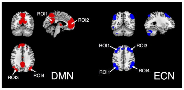
ROI atlases of the DMN and ECN (network templates downloaded from http://findlab.stanford.edu/functional_ROIs.html).

To obtain a more comprehensive view on the frequency characteristic of the correlated BOLD-like components, ‘correlated signal amplitude vs. TE’ linear regression (see section 2.1.5 correlated signal vs. TE above) was further performed at each specific frequency instead of divided bands, and the fitted slope β(f) at each frequency f was taken to reflect the signal amplitude of BOLD-like component. To suppress ill-conditioned estimation of β(f) due to noise, a Tikhonov regularization was applied using eqn. (3):

$${\text{argmin}}_{\mathrm{\alpha },\mathrm{\beta }}\left\{\left({\mathrm{\sum }}_{f\epsilon [00.5]Hz}{\mathrm{\sum }}_{TE=5~30ms}{\Vert S_{c,TE}(f)-\alpha (f)-TE·\beta (f)\Vert }_2^2\right)+\mathrm{\lambda }({\Vert \alpha \Vert }_2^2+{\Vert \beta \Vert }_2^2)\right\}$$ (3)

where S_c,TE(f) denotes the correlated signal amplitude at frequency f and echo time TE, α(f) and β(f) denote the intercept and slope term in eqn. (2). Unlike previous analysis where all the subjects’ data were combined for a single model fitting, this analysis was performed for individual subjects separately. In this analysis we set λ = 1, and the subject mean of the fitted BOLD-like component did not change prominently for λ ∈ [10⁻⁷ 10¹].

2.2 Model of the RS HRF

The HRF in the resting state was modeled based on Buxton’s balloon model (Buxton et al., 1998), with implementation and parameters adapted for 3T (Mildner et al., 2001). To mimic RS, a negligible flow input was entered into the non-linear system (two differential equations charactering the changes of deoxygenated hemoglobin concentration and vessel volumes). The equations are listed in Appendix C Equations for RS HRF simulation, and detailed parameters of the simulation are listed in Table 1. The difference in our calculation therefore lies in assuming only small perturbations from the baseline condition rather than the large in-flow modeled for task-evoked conditions.

Table 1.

Summary of the parameters used to simulate the rest HRF. Balloon model parameters were selected based on the values reported in previous literature – ((Mildner et al., 2001) for α τ₀, τ_v, k1, k2, k3) and ((Buxton et al., 2004) for E₀, V₀).

	Parameters		Values
Inflow (a trapezoid)	Ramp time		0.1 s
	Maximum amplitude		1.05
	Plateau time		1 s
Balloon Model Parameters	α (steady-state flow-volume relation: v = fα)		0.3~0.6
	τv (a viscosity parameter depicting an additional resistance to rapid volume changes during undershoot)		25~35 (s)
	τ0 (mean transit time through the venous compartment at rest)		1.8~2.5 (s)
	E0 (Baseline O2 extraction fraction)		0.4
	V0 (Baseline blood volume)		0.03
	Dimensionless parameters quantifying the BOLD contributions from different components	k1	6.7
		k2	2.73
		k3	0.57

2.3 Seed-based correlation

Pre-processed data were temporally filtered into two distinct frequency bands: (<0.1 Hz) and (0.2~0.4 Hz). The spatial patterns of RS networks within the two frequency bands were derived using seed-based Pearson correlation, and voxels with peak ICA z-scores in the posterior cingulate cortex (PCC) region and amongst all the regions in the ECN map from ICA were chosen as the network seeds for DMN and ECN separately.

3 Results

3.1 TE-dependence of correlated signal amplitude

Fig. 2 plots the correlated signal amplitude as a function of TE in the six different frequency bands: 0~0.5 Hz (B0), 0.01~0.1 Hz (B1), 0.1~0.2 Hz (B2), 0.2~0.3 Hz (B3), 0.3~0.4 Hz (B4), and 0.4~0.5 Hz (B5). Signals across all frequency bands exhibited a significantly linear dependence on TE, demonstrating persisting BOLD-like contributions to RSFC at frequency bands above the conventional 0.1 Hz. However, intercepts of the fitted linear models deviated from the theoretical zero, and were frequency dependent and more prominent in higher frequency bands (see Table 2 for the statistical significance of fitted intercepts, and Fig. 3 for the ratio of fitted intercepts and slopes – the ratio at B5 is ~4 times that of B1), implying increased contributions from non-BOLD-contrast relative to BOLD contrast at higher frequencies.

Fig. 2.

Functional connectivity signal amplitudes vs. TE. Statistics shown here are standard linear model vs. Gaussian noise tests; lack-of-fit tests were also performed and failed to reject the linear hypothesis for all frequency bands (not shown). To account for the inter-subject variability, each subject’s correlated signal amplitudes were first normalized (divided by the mean correlated amplitude across different TEs of B0 band) before group fitting.

Table 2.

Summary of the statistical significance (p-values) of the fitted intercepts (conventional t test of the estimated covariates in a linear regression). ‘Voxel-pairs’: fitted results using between-voxel covariance as correlated signal amplitude; ‘ROI-pairs’: fitted results using covariance between network ROIs as correlated signal amplitude; ‘Reproducibility’: fitted results in the reproducibility test (datasets from four subjects acquired in separate scans) using between-voxel covariance as correlated signal amplitude. ‘Trial 1’: data collection from the 1^st trial of the experiment; ‘Trial 2’: data collection from the 2^nd trial of the experiment.

		0–0.5 Hz	0.01–0.1 Hz	0.1–0.2 Hz	0.2–0.3 Hz	0.3–0.4 Hz	0.4–0.5 Hz
Voxel-pairs	DMN	2.8e-5	9e-4	1.4e-3	4.3e-3	1.1e-6	7e-7
	ECN	1.4e-6	3.1e-4	1.4e-4	4e-3	1.8e-4	1.8e-5
ROI-pairs	DMN	0.051	0.128	4e-3	0.038	1.1e-4	1.2e-4
	ECN	0.030	0.443	8.3e-4	5.1e-4	1.5e-6	8e-6
Reproducibility	Trial1	6.7e-7	1.7e-4	0.039	7.9e-4	4.2e-6	2.9e-8
	Trial2	4e-3	9e-3	0.015	0.36	0.025	8e-3

Fig. 3.

Ratios of fitted intercepts (non-BOLD contrast) over slopes (BOLD contrast), suggesting increased importance of non-BOLD contributions at higher frequencies; see Table 2 for descriptions of ‘Voxel-pairs’, ‘ROI-pairs’, ‘Reproducibility’.

A paired-t test (α = 0.05) revealed no significant difference between the fitted parameters from two separate sets of scans except the fitted slope of (0.1~0.2 Hz) (p = 0.0386, uncorrected). At the group level (correlated signal amplitudes of different subjects were combined and regressed against TE), results turned out to be remarkably reproducible, as revealed by the comparison of two separate scans from subjects who were scanned twice (see Fig. 3, supplementary Fig. S1).

Results estimated using signals from separate ROIs were qualitatively similar – spontaneous FC exhibited linear TE-dependence in all the frequency bands and increasing fractions of non-BOLD-like contributions were present at higher frequencies, although there were quantitative differences in the values of fitted slopes and intercepts (see Table 2, Fig. 3, supplementary Fig. S2).

Figures 4E, 4F show the frequency characteristics of BOLD-like signal amplitudes within DMN and ECN respectively. Consistent with prior RS studies, the power spectrum primarily encompasses frequencies < 0.1 Hz, and signals decay fast at higher frequencies but the amplitude (the slope of the TE-dependence of signal) appears to reach a non-zero asymptote up to 0.5 Hz.

Fig. 4.

(A) Conventional HRFs and (B) frequency responses; (C) Simulated RS-HRFs and (D) frequency responses; (E, F) BOLD signal amplitudes (fitted slopes, BOLD-like contrast only) vs. frequency estimated from experimental data for DMN and ECN, respectively, normalized by the maximum amplitude of subject mean. As predicted, BOLD signal amplitudes dropped dramatically with frequency, but were still nonzero at the highest frequency (0.5 Hz).

3.2 HRF at rest

The simulated RS HRFs (see section 2.2 Model of the RS HRF) and their corresponding frequency responses for the range of parameters in Table 1 are shown in Figs. 4C and 4D, respectively. Compared with the HRF models during task conditions where large changes in capillary flow into the venous outflow tract are assumed (Figs. 4A, 4B), the RS waveforms have accelerated signal rise and recovery as well as diminished undershoot – resulting in elevated frequency responses at 0.3 Hz (and beyond to ~1 Hz). If we further contrast modeled frequency characteristics of HRFs at task and rest conditions (Figs. 4B, 4D) with measured BOLD spectral characteristics (Figs. 4E, 4F), we note that the RS HRF model more reasonably supports the BOLD spectra estimated from experimental data than does the task HRF (Figs. 4A, 4B) : Under the roughly linear assumptions of the hemodynamic process (Boynton et al., 1996; Dale and Buckner, 1997), non-zero system outputs (Figs. 4E, 4F) above 0.3 Hz requires non-zero response of the system transfer function (HRF in the stable hemodynamic system) in the corresponding frequency range. It is important to note that without changing the fundamental Balloon model design, but simply running the model at baseline conditions rather than elevated RCBF, the frequency response is elevated enough to support the measured BOLD fluctuations at high frequencies. These results suggest the need to utilize different HRF models under task and RS conditions.

3.3 Seed-based RS functional connectivity

Fig. 5 shows the RS connectivity patterns from the seed-based correlation analysis (see section 2.3 above) in representative subjects at two non-overlapping frequency bands (<0.1 Hz) and (0.2~0.4 Hz); correlation maps were smoothed by a Gaussian kernel (FWHM = 4 mm) before display. Results of the remaining subjects are displayed in supplementary Figs. S3, S4. FC <0.1 Hz exhibited robust RSN patterns as reported in previous literature (Greicius et al., 2003; Shirer et al., 2012) in all the examined subjects, while connectivity patterns between 0.2~0.4 Hz were observable in a subset of subjects, as shown in Fig. 2 and supplementary Figs. S3, S4. Notably, although RSFC persisted at higher frequency range in certain subjects, the spatial patterns were frequency dependent: for instance, in the DMN of sub02, the correlation of dorsolateral prefrontal cortex and the PCC seed was significantly negative at frequency bands below 0.1 Hz, but became significantly positive between 0.2~0.4 Hz, as indicated by white circles (Fig. 5A).

Fig. 5.

DMN/ECN patterns of representative subjects at <0.1 Hz (upper rows) and 0.2~0.4 Hz (bottom rows) (|r|>0.2, p<0.002, uncorrected). The power spectra of the chosen network seed signals at (<0.1 Hz) and (0.2~0.4 Hz) are highlighted in blue and red separately. Numbers in the parenthesis indicate the scan trial for subjects who participated twice.

To further quantify the similarity of RS network patterns at different frequency bands, we introduced a similarity measure POV as follows:

$$\text{Percentage}\text{of}\text{overlapped}\text{voxels}(\text{POV})=\frac{({\mathit{CorrMap}}_{<\mathit{0.1}Hz})\cap ({\mathit{CorrMap}}_{\mathit{0.2}~\mathit{0.4}Hz})}{({\mathit{CorrMap}}_{<\mathit{0.1}Hz})\cup ({\mathit{CorrMap}}_{\mathit{0.2}~\mathit{0.4}Hz})}$$

where CorrMap refers to the thresholded correlation map. The POV similarity between network patterns derived at different frequencies is shown in Fig. 6A. Among all the results associated with DMN and ECN, the maximum POV is only ~ 50%, reflecting inconsistent spectral behaviors of spontaneous activity in general. Moreover, the curves of ‘POV vs. thresholds’ (dashed blue lines) vary largely across subjects, implying non-negligible inter-subject variability in frequency specificity of spontaneous FC.

Fig. 6.

(A) The POV (percentage of overlapped voxels) similarity index between the high-frequency RSFC pattern (0.2~0.4 Hz, thresholded at r = 0.15) and the low-frequency RSFC pattern (<0.1 Hz, thresholds were varied from 0 to 0.8). Each dashed blue line represents the result of one single scan. Dark line presents the mean; (B) The number of voxels with significant positive/negative correlations with PCC (p < 0.05, |r|>0.13, uncorrected) at different frequency bands, the numbers of voxels significantly anti-correlated with PCC (blue) are multiplied by ten to contrast those associated with positive correlations (red) on the same legend scale; error bars are the standard deviations across subjects.

We also counted the number of voxels with significant positive/negative correlations within DMN (p < 0.05, |r| > 0.13, uncorrected) for each subject, as shown in Fig. 6B. Compared to correlations estimated utilizing the whole frequency band, both positive and negative correlations were amplified in the restricted band <0.1 Hz, and diminished at 0.2~0.4 Hz. In particular, anti-correlations were strongly attenuated in higher frequency bands for all the examined subjects.

3.4 Noise and SNR as a function of frequency

Results presented above (Figs. 2, 4E, 4F) suggest that although spontaneous activity persisted at frequencies above 0.1 Hz, the amplitude still decays quickly as a function of frequency. Hence, to support the observed functional connectivity at higher frequency bands, residual noise must also decay as a function of frequency to compensate. Fig. 7A shows the amplitudes of signals (the correlated part of the raw signals) and noise (uncorrelated residuals) across different frequency bands estimated from ROI signal pairs (see Fig. 1), and both decrease quickly as frequency increases. As a result, the SNR, which is tightly coupled to correlation amplitude, exhibits a milder decay compared to BOLD amplitudes themselves (Fig. 7B). Indeed, the SNR at B5 (0.4–0.5 Hz) is ~50% that at B1 (0.01~0.1 Hz), while the corresponding signal ratio is only ~ 13%.

Fig. 7.

(A) Correlated signal amplitudes (averaged across ROI signal pairs) and noise amplitudes (root mean square of the uncorrelated residuals, also estimated from ROI signal pairs) at different frequency bands; each dot represents the result from a single scan (scans with TE = 25 and 30ms are displayed). (B) SNR as a function of frequency bands.

3.5 Influences of distinct HRF spectral characteristics on the spatial pattern of functional connectivity

If regions within the same RS network are characterized by different HRFs (both amplitudes and the frequency responses), the evoked responses across brain regions will naturally exhibit distinct intensity patterns at different frequencies even though the underlying neuronal mechanisms (system input) may be spatially-invariant, and may further result in frequency-dependent correlation patterns when contaminated by noise with disproportional spectral characteristics.

To examine the potential confounds from inconsistent HRF shapes (frequency characteristics) inside a RS network on the exhibited network pattern, we take signals inside the DMN 0f sub01(2) (Fig. 8B) as an example for further analysis. The recently proposed blind de-convolution approach (Wu et al., 2013) was employed to estimate the rest HRFs of each ROI (HRFs were fitted with bases shown in Fig. 8A). De-convolution resulted in heterogeneous HRFs across ROIs (Fig. 8C) and differences in intensity patterns across frequency bands (shown in Fig. 8D, where the intensity of ROI1 was nearly identical with ROI4 < 0.1 Hz, while prominently higher than ROI4 within 0.2~0.4 Hz, as indicated by red arrows). We therefore performed further simulations to examine the influence of HRF inconsistency across regions on the frequency characteristics of the overall networks. In the simulation, we assumed periodic autonomic neuronal stimuli at two distinct periods — 3s (‘Event1’) and 15s (‘Event2’) (Fig. 8 E ‘events’), and signals from different ROIs were simulated by convolving the stimulus with the estimated HRFs (Fig. 8E, ‘Simulated signals’) and temporally filtered (0.2~0.4 Hz for ‘Event1’, < 0.1 Hz for ‘Event2’) to remove higher order harmonics. Raw noise terms were generated from randomly permuted versions of the fitted residuals from the HRF estimation. To mimic the frequency-dependence of SNR in real data (Fig. 7), the raw noise was temporally filtered into two bands (<0.1 Hz, SNR ~1.40 and 0.2~0.4 Hz, SNR ~ 0.74) and scaled separately based on the mean standard deviation of the simulated signal amplitudes across ROIs (i.e. noise levels of different ROIs were identical) and SNR at the corresponding band. Contrasting the correlation matrixes of the ROIs under different stimulus conditions (Fig. 8E Correlation matrix, top, 0.2~0.4 Hz, bottom, <0.1 Hz) clearly demonstrates differences in the patterns. For instance, correlation between ROI 4–5 was higher than ROI 1–5 below 0.1 Hz, but the comparison was inverted in 0.2~0.4 Hz band (indicated with red arrows), which was attributable to the changes of intensity patterns shown in Fig. 8D. Imagining the simulated neuronal stimulus being an additive mixture of ‘Event1’ and ‘Event2’, data correlation at filtered bands would therefore exhibit distinct correlation structure as shown here.

Fig. 8.

The influence of heterogeneous HRFs within a RS network on the frequency specificity of the exhibited network patterns. (A) Basis functions employed in HRF fitting: canonical HRF (blue), temporal derivative (green), dispersive derivative (red); (B) ROIs within the DMN (sub01 (2)) chosen for simulations; (C) Estimated HRFs and the normalized frequency responses; (D) Frequency specificity of signal intensity patterns (un-normalized response power of estimated HRFs in (C) integrated within the corresponding frequency bands); (E) Disparate correlation patterns of simulated signals (‘Simulated signals‘) (shown by ‘Correlation matrix’) with stimulus input (‘Events’) given at different frequency scales.

It may appear contradictory that we have suggested modifications of hemodynamic models at rest, but still adopted the bases from task models (Fig. 8A) to de-convolve RSFC data to generate rest HRFs (Fig. 8C). However, for task models, the coefficients fit for the amplitude of the three bases in the general linear model must have a specific relationship so that the linear approximation of 1^st order derivative can hold. Here, we relaxed such constraints, and only set |β_dispersion | ≤ 0.5β_canonical to enforce reasonable shapes of fitted HRFs (no double overshoots), which resulted in more flexible waveforms and extended frequencies beyond 0.3 Hz (Fig. 8C). Of note, the simulations performed here do not aim to justify the validity of the blind de-convolution approach (the fitted HRFs indeed deviate from the shapes simulated with Buxton’s model (cf. Fig. 4C)), but rather to generate versatile HRFs within a RS network in order to demonstrate that frequency specificity of RSFC may also source from a non-stationary vascular origin.

4 Discussion

4.1 BOLD-like contributions to RSFC above 0.1 Hz

With TR = 1s, we observed salient linear dependence of correlated signal amplitudes on TE at frequency bands up to 0.5 Hz within the DMN/ECN, demonstrating persistence of BOLD-like RSFC at frequencies above 0.1 Hz.

The apparent contradiction between predictions from the conventional HRF model (Fig. 4B) and BOLD-like signals at frequency bands up to 0.5 Hz (Figs. 4E, 4F) implies that canonical task HRFs may not be applicable to rest conditions, where the cerebral blood flow exhibits only small fluctuations about equilibrium. Simulations using Buxton’s balloon model at equilibrium extends the limit of observable BOLD responses to nearly 1 Hz (Fig. 4D), and the simulated HRFs (system transfer functions) qualitatively support the experimental results in Figs. 4E,F (fitted slope of correlated signal amplitudes as a function of frequency, viewed as system outputs). To our knowledge, a distinction between the HRF during task and in RS has not been proposed before. While our extension of Buxton’s balloon model to RS conditions may need further refinement, these simulations demonstrate that higher frequency BOLD signal changes can be predicted than is expected from current models as the strength of stimulus input approaches equilibrium. Qualitatively, because the outflow tract —balloon is in equilibrium rather than distended by a bolus of deoxygenated blood from an evoked metabolic response, there is negligible signal undershoot and a more rapid response to small perturbations in blood flow.

Of note, although the modified RS HRF apparently supports BOLD responses in frequency bands up to 1 Hz, the BOLD spectrum still decays quickly due to the inherently sluggish nature of perfusion through the capillary bed. Despite this decrease in signal at higher frequencies, the persistence of significant functional connectivity in the high frequency correlation patterns (Fig. 5 and supplementary Figs. S3, S4) suggest that residual noise must also decay as a function of frequency to compensate, as was proposed by (Lee et al., 2013) and demonstrated in Fig. 7 of the present datasets.

Although the spectral behavior of the uncorrelated noise residuals (Fig. 7A noise) is in accordance with the wide prevalence of ‘1/f’-like noise found in nature, and specifically in fMRI signals (Bullmore et al., 2001; He, 2011), further exploration into the confounding sources of noise may provide additional insights into the mechanisms underlying FC structures at different frequency scales. For instance, it is possible that RSFC at the lower frequency range meditates the general excitability (Raichle, 2011) and distinct RS networks that are spatially overlapped (Smith et al., 2012), while RSFC at the higher frequency ranges may be confined to focal functions. Thus, an ROI in one RS network (RSN1 for instance) may contain slow fluctuations synchronized with the principal activity associated with a different network (say RSN2) but uncorrelated with the temporal behavior of the other ROIs inside RSN1. It is also possible that fluctuations and FC at low-frequency may derive largely from the maintenance of basic hemodynamic stasis that is controlled by the parasympathetic nerve system rather than by fluctuations in neural metabolism. If that is so, then higher frequency FC may offer a more direct and precise characterization of cognitive processes than the typical low-pass filtered FC analyses.

4.2 non BOLD-like contributions to RSFC above 0.1 Hz

As demonstrated in Fig. 2, the correlated signal amplitude remains positive as TE approaches zero at all frequencies, which deviates from the theoretical BOLD model. The ratio of the fitted intercepts to the slopes further suggests more prominent fractional contributions from the non-BOLD-like components to RSFC at higher frequency ranges (see Fig. 3). One possible mechanism is blood inflow (Gao and Liu, 2012), however this contribution is most prominent with heavy T1 weighting and not likely to be appreciable at the 1s TR employed here. An alternate contrast mechanism that is most important as TE approaches 0, that of proton density weighted imaging is Signal Enhancement by Extravascular water Protons (SEEP), which reflects endogenous proton-density changes associated with astrocyte swelling and increased tissue water content in active neural tissue (Figley et al., 2010). This alternative mechanism underlying fMRI changes was first identified in spinal cord imaging (Stroman et al., 1999) and extended to brain areas later (Stroman et al., 2001). It has been postulated to account for the non-zero extrapolates at TE = 0 in multi-TE experimental results resembling current observations (Stroman et al., 2001). Moreover, as a direct measure of the endogenous change of proton density (signals may exhibit no clear favor in specific frequency bands), it is in good accordance with the extended correlations in higher frequency range (see Figs. 4E, F). However, due to the long TR required for acquisition of proton-density weighted images, resolving SEEP contrast at higher temporal scales is challenging. Accordingly, without further experimental evidence, the interpretation proposed here is speculative.

Another potential source for non-BOLD functional connectivity relates to the physiological noise, which has been demonstrated by (Kruger and Glover, 2001) to contain both BOLD-like components (caused by the same mechanism that induces changes in R₂*) and non-BOLD-like image-to-image signal fluctuations due to cardiac/respiratory functions. Although physiological corrections (Glover et al., 2000; Chang et al., 2009) were applied to the datasets, residuals may still persist and contribute to the non-TE dependency of the RS functional connectivity. There are two arguments against this hypothesis: (1) as revealed by the spatial patterns of DMN/ECN at higher frequency bands (Figs. 5, S3, S4), functional connectivity is mainly confined to standard DMN/ECN regions, whereas cardiac noise manifests primarily near large vessels and respiratory noise is more global; (2) it is unclear how non-BOLD physiological contributions can become more prominent at higher frequencies. Similarly, we exclude potential confounds from subjects’ motion because: (1) the motion was small (root-mean-square of translational movements = 0.26±0.11mm across all 66 scans), and (2) motion regressors were employed as nuisance covariates. Thus, head motion is unlikely to contribute greatly to the observed non-BOLD functional connectivity.

4.3 Inconsistent network patterns across frequency bands

The spatial patterns of RSFC were found to be frequency-dependent (Figs. 5, 6, supplementary Figs. S3, S4), which is in line with the results reported by other groups (Boubela et al., 2013; Gohel and Biswal, 2014; Niazy et al., 2011; Wu et al., 2008). If such frequency specificity relates to different aspects of neural activity, as has been hypothesized here and by others, promising avenues for future analysis may involve characterizing the correspondence of distinct frequency bands of fMRI data and different rhythms of electrophysiological recordings (Buzsaki and Draguhn, 2004; Chang et al., 2013; Laufs et al., 2006; Mantini et al., 2007; Raichle, 2011; Yuan et al., 2012).

However, it has been demonstrated that the shapes of HRF, which depend on vessel diameters and structures, are heterogeneous across different brain areas even though these areas are functionally coupled (see (Buxton, 2012; Handwerker et al., 2012; Menon, 2012) for reviews). Such inconsistency of HRF shapes may likely contribute to the observed frequency specificity of RSFC, as demonstrated in Fig. 8.

Given that regional HRFs may plausibly have disparate spectral responses, our observation of inter-subject variability in the spatial patterns of RS networks (Figs. 5, 6A, supplementary Figs. S3, S4) may relate to these regional HRF differences rather than the more commonly assumed inconsistent functional organizations across subjects. This suggests that more careful analyses of RSFC should include consideration of latency (Chang et al., 2008) and shape changes in the HRF across nodes of the networks.

Another study finding is that negative correlations were barely observable at 0.2~0.4 Hz (Figs. 5 and 6B), which may require positing a distinct neuronal mechanism at higher frequency, or by the possibility that negative interactions may undergo inherently slower hemodynamic processes.

We further note that while the temporal resolution of fMRI acquisitions may continue to increase through technical improvements, the spatial- and subject-variable nature of HRFs may act as a ‘frequency domain smoother’, and limit our capability to generalize quantitative results at very finely divided frequency intervals, say average bandwidth of 0.05 Hz or even narrower (Wu et al., 2008).

4.4 Further technical considerations

Unlike multi-echo acquisition as performed by (Kundu et al., 2012; Peltier and Noll, 2002), we collected RS datasets with different TEs in separate scans, overlooking the fact that subjects’ states may vary over time. To assess the data consistency across scans, an additional 6-min RS scan with a randomly chosen TE was performed at the end of the 6 RS scans in a subset of experiments: sub04(1) 20ms, sub05 25ms, sub06(1) 5ms. For all the examined cases, the correlated amplitude estimated from the additional scan agreed well with that of a prior scan with identical TE parameter (data not shown).

With TR = 1s, our data acquisition only supported the examination of spontaneous activity up to 0.5 Hz. However, both the simulated RS HRF (Figs. 4C, 4D) and the observed BOLD spectra (Figs. 4E, 4F) imply the presence of functional connectivity at even higher frequency range (Boubela et al., 2013; Lee et al., 2013), which inspires the potential concern that these observations may contain aliased components from frequencies above 0.5 Hz. Although the major discoveries and questions inspired by the study are not violated, the quantitative results presented here may require cautious interpretation and warrant further examination with data acquisition at much faster sampling rate.

Of note, most analyses herein focused on the intra-scan comparison of functional connectivity across different frequency bands (Figs. 2, 4, 5A), and a 6-min scan (360 time points with TR = 1s) should be long enough to provide adequate degrees of freedom (even considering temporal autocorrelation) to yield reliable conclusions on functional correlation/covariance. However, for studies attempting to generate reliable measures of the spatial patterns of RS functional connectivity across different frequency bands, longer scan durations (9~13 min as suggested by (Birn et al., 2013)) may be needed to encompass enough cycles of slow frequency network dynamics.

To resolve RSFC at higher frequency bands, fMRI protocols with faster sampling rates are needed. However, accompanying the increased number of sample points acquired and increase in degrees of freedom in a fixed scan duration is the decreased correlation threshold for a given p-value (assuming the null distribution unaltered): the lower bound of significant correlation r (p<0.05, uncorrected) drops from 0.15 at TR = 2s to 0.055 at TR = 0.1s for a 6-min long scan (using an AR(1) autocorrelation model). An effect of the lowered threshold is that the results become more sensitive to non-neural-activity-relevant correlations incurred by non-random sources, say motion at sub-periods of a scan etc. Also noteworthy is the ‘expansion’ of actual correlation introduced by spatial smoothing may become more prominent given the lowered statistical threshold. Although smoothing has been widely adopted to enhance local SNR and mitigate the bias between inherent noise structure of real data and the assumed model in conventional RS analysis (Friston et al., 2000), it is worthwhile to reconsider the feasibility to extend identical preprocessing to RS data collected at higher frequencies, which may be of particular relevance for studies attempting to examine persisted RSFC within a focal region (say visual cortex in (Lee et al., 2013; Wu et al., 2008)) instead of between remote brain areas.

Another technical concern involves the approach employed to extract the RS networks across different frequency bands – the majority of studies looking at RSFC have been relying on the results generated by either ICA (Beckmann et al., 2005; Smith et al., 2009) or seed-based correlation (Biswal et al., 1995). Although prior studies have demonstrated that, with ICA, one is able to produce similar network patterns generated by conventional seed-based correlation approach (Greicius et al., 2004), it is worth noting that ICA differs fundamentally from linear correlation – various ICA algorithms only enforce the output spatial maps to be sparse and statistically independent (see (Beckmann, 2012) for different algorithms defining independence). Therefore, it is possible to observe disparate network patterns using different analysis approaches, which may likely be the case especially in higher frequency bands: in the case for ICA, with the drop of SNR (see Fig. 7) and possibly more complicated mixture of un-identified signal sources as proposed hereby, the performance of ICA is yet unclear; moreover, in the case of seed-based correlation, locations of network hubs (seeds) may be frequency dependent as well (Lee, 2014), and optimum seed location across frequency bands may vary. Indeed, in (Gohel and Biswal, 2014), the authors observed certain discrepancies between these two approaches: for instance, networks resolved by ICA exhibited more variable spatial patterns across frequency compared to the seed-based correlation approach.

5 Conclusion

This fMRI study provides further evidence supporting the persistence of RSFC at frequency bands higher than 0.1 Hz and the differences in network patterns across different frequencies. With acquisition at different TEs, we have observed BOLD-like linear dependence of spontaneous activity on TE, supporting neural relevance of the RSFC in extended frequency bands and implying that HRF models should be modified for rest compared to traditional task-based models. We have also demonstrated considerable contributions to the FC signals, particularly in higher frequency bands, from TE-independent components in the examined two networks, although whether these signals originate from neural activity instead of confounding noise sources remain unclear. Given the very limited knowledge of spontaneous activity above 0.1 Hz at the current stage, mechanisms underlying the present observations are not yet conclusive, which may be of great interest to query in future studies.

Highlights.

• Resting-state functional connectivity (RSFC) persist above 0.1 Hz

• Observe BOLD-like linear TE-dependence in spontaneous activity up to 0.5 Hz

• Increased fractions of non-BOLD-like signal contributions to RSFC above 0.1 Hz

• HRF models at task conditions must be modified at rest

• Spatial patterns of RSFC are frequency-dependent

Appendix A Schemes to generate the RS network masks from ICA results (for each subject separately)

1. Identify the independent components (IC) resembling the spatial patterns of DMN/ECN by visual inspection. In cases where ECN was separated into left ECN (LECN) and right ECN (RECN), both ICs were selected;

2. Threshold the IC maps to generate a preliminary mask of each network, thresholds were tuned so that 300~500 voxels remained in the mask (LECN and RECN were thresholded separately and combined as a unified mask);

3. Average fMRI time series within each preliminary network mask and linearly correlate the averaged signal to voxels across the brain for all the six scans with different TEs;

4. Joint voxels of thresholded correlation maps (correlation coefficient r > 0.2, and 0.15 for subjects with generally weaker correlations) from scans with TE = 15, 20, 25, 30 ms were taken as the final network mask. Thresholds of correlation coefficients ranging from 0.1 to 0.25 resulted in very minor effects on the results, because the results associated with each subject were first normalized before ensuing group analysis (section 2.1.5 Correlated signal amplitude vs. TE).

Appendix B Computation of between-voxel covariance across different frequency bands

Let {x_i}_1≤i≤N, {y_i}_1≤i≤N, denote two demeaned time series, and ${\{x_i^B\}}_{1\le i\le N},{\{y_i^B\}}_{1\le i\le N}$ denote the filtered time series within frequency band B.

Based on the Plancherel theorem, the covariance of ${\{x_i^B\}}_{1\le i\le N}$ and ${\{y_i^B\}}_{1\le i\le N}$

$$\mathit{Cov}(x^B,y^B)=\frac{\mathit{1}}{N-\mathit{1}}{\sum }_{i=1}^N{x}_i^B·y_i^B$$ [B.1]

equals to

$$\frac{1}{N-1}·\frac{1}{N}{\sum }_{k=1}^N{X}_k^B·\overline{Y_k^B}=\frac{1}{N-1}·\frac{2}{N}{R}_e\left({\sum }_{1\le l\le N,\frac{l}{N}{f}_s\in B}{X}_l·{\overline{Y}}_l\right)$$ [B.2]

where f_s is the sampling rate (1/TR), {X_k}_1≤k≤N, {Y_k}_1≤k≤N, ${\{X_k^B\}}_{1\le k\le N},{\{Y_k^B\}}_{1\le k\le N}$ correspond to the DFT series of {x_i}_1≤i≤N, {y_i}_1≤i≤N ${\{x_i^B\}}_{1\le i\le N},{\{y_i^B\}}_{1\le i\le N}$ respectively, R_e refers to the real part of a complex number.

Appendix C Equations for RS HRF simulation

The simulation was conducted using equations presented in (Mildner et al., 2001), which provided a modified version of Buxon’s balloon model (eqn. C1):

$$\begin{array}{c}\stackrel{.}{q}(t)=\frac{\mathit{1}}{{\tau }_{\mathit{0}}}\left\{f_{in}(t)\frac{E(t)}{E_{\mathit{0}}}-f_{\mathit{out}}(v)\frac{q(t)}{v(t)}\right\}\\ \stackrel{.}{v}(t)=\frac{\mathit{1}}{{\tau }_{\mathit{0}}}\left\{f_{in}(t)-f_{\mathit{out}}(v)\right\}\end{array}$$ [C1]

where the total deoxyhemoglobin content q(t), the blood volume v(t), inflow function f_in(t) and outflow function f_out(v) are scaled by their values at rest. q̇(t) and v̇(t) denote the temporal derivative of q(t) and v(t) separately. τ₀ denotes the mean transit time estimated by the ratio of the blood volume to blood flow at rest, E₀ denotes the baseline O₂ extraction fraction, and E(t) = 1−(1−E₀)^1−f_in(t).

The relationship between f_out and ν is modeled as:

$$f_{\mathit{out}}(v)=v^{\mathit{1}/\alpha }+{\tau }_v\frac{dv}{dt}$$ [C2]

where τ_v is an additional resistance to the rapid volume change.

Assuming τ₀ ≤ τ_v, eqn. [C1] can be approximated by:

$$\begin{array}{c}\stackrel{.}{q}(t)=\frac{f_{in}(t)}{{\tau }_{\mathit{0}}}\left\{\frac{E(t)}{E_{\mathit{0}}}-\frac{q(t)}{v(t)}\right\}+\frac{\mathit{1}}{{\tau }_v}\left\{f_{in}(t)-v^{\mathit{1}/\alpha }\right\}\frac{q(t)}{v(t)}\\ \stackrel{.}{v}(t)=\frac{\mathit{1}}{{\tau }_v}\left\{f_{in}(t)-v^{\mathit{1}/\alpha }\right\}\end{array}$$ [C3]

References

- Beckmann CF. Modelling with independent components. NeuroImage. 2012;62:891–901. doi: 10.1016/j.neuroimage.2012.02.020. [DOI] [PubMed] [Google Scholar]
- Beckmann CF, DeLuca M, Devlin JT, Smith SM. Investigations into resting-state connectivity using independent component analysis. Philosophical Transactions of the Royal Society B-Biological Sciences. 2005;360:1001–1013. doi: 10.1098/rstb.2005.1634. [DOI] [PMC free article] [PubMed] [Google Scholar]
- Birn RM, Molloy EK, Patriat R, Parker T, Meier TB, Kirk GR, Nair VA, Meyerand ME, Prabhakaran V. The effect of scan length on the reliability of resting-state fMRI connectivity estimates. Neuroimage. 2013;83:550–558. doi: 10.1016/j.neuroimage.2013.05.099. [DOI] [PMC free article] [PubMed] [Google Scholar]
- Biswal B, Yetkin FZ, Haughton VM, Hyde JS. Functional connectivity in the motor cortex of resting human brain using echo-planar MRI. Magn Reson Med. 1995;34:537–541. doi: 10.1002/mrm.1910340409. [DOI] [PubMed] [Google Scholar]
- Boubela RN, Kalcher K, Huf W, Kronnerwetter C, Filzmoser P, Moser E. Beyond Noise: Using Temporal ICA to Extract Meaningful Information from High-Frequency fMRI Signal Fluctuations during Rest. Front Hum Neurosci. 2013;7:168. doi: 10.3389/fnhum.2013.00168. [DOI] [PMC free article] [PubMed] [Google Scholar]
- Boyacioglu R, Beckmann CF, Barth M. An Investigation of RSN Frequency Spectra Using Ultra-Fast Generalized Inverse Imaging. Front Hum Neurosci. 2013;7:156. doi: 10.3389/fnhum.2013.00156. [DOI] [PMC free article] [PubMed] [Google Scholar]
- Boynton GM, Engel SA, Glover GH, Heeger DJ. Linear systems analysis of functional magnetic resonance imaging in human V1. J Neurosci. 1996;16:4207–4221. doi: 10.1523/JNEUROSCI.16-13-04207.1996. [DOI] [PMC free article] [PubMed] [Google Scholar]
- Bullmore E, Long C, Suckling J, Fadili J, Calvert G, Zelaya F, Carpenter TA, Brammer M. Colored noise and computational inference in neurophysiological (fMRI) time series analysis: resampling methods in time and wavelet domains. Hum Brain Mapp. 2001;12:61–78. doi: 10.1002/1097-0193(200102)12:2<61::AID-HBM1004>3.0.CO;2-W. [DOI] [PMC free article] [PubMed] [Google Scholar]
- Buxton RB. Dynamic models of BOLD contrast. NeuroImage. 2012;62:953–961. doi: 10.1016/j.neuroimage.2012.01.012. [DOI] [PMC free article] [PubMed] [Google Scholar]
- Buxton RB, Wong EC, Frank LR. Dynamics of blood flow and oxygenation changes during brain activation: the balloon model. Magn Reson Med. 1998;39:855–864. doi: 10.1002/mrm.1910390602. [DOI] [PubMed] [Google Scholar]
- Buxton RB, Uluda K, Dubowitz DJ, Liu TT. Modeling the hemodynamic response to brain activation. NeuroImage. 2004;23:220–233. doi: 10.1016/j.neuroimage.2004.07.013. [DOI] [PubMed] [Google Scholar]
- Buzsaki G, Draguhn A. Neuronal oscillations in cortical networks. Science. 2004;304:1926–1929. doi: 10.1126/science.1099745. [DOI] [PubMed] [Google Scholar]
- Chang C, Cunningham JP, Glover GH. Influence of heart rate on the BOLD signal: the cardiac response function. NeuroImage. 2009;44:857–869. doi: 10.1016/j.neuroimage.2008.09.029. [DOI] [PMC free article] [PubMed] [Google Scholar]
- Chang C, Liu Z, Chen MC, Liu X, Duyn JH. EEG correlates of time-varying BOLD functional connectivity. NeuroImage. 2013;72:227–236. doi: 10.1016/j.neuroimage.2013.01.049. [DOI] [PMC free article] [PubMed] [Google Scholar]
- Chang C, Thomason ME, Glover GH. Mapping and correction of vascular hemodynamic latency in the BOLD signal. NeuroImage. 2008;43:90–102. doi: 10.1016/j.neuroimage.2008.06.030. [DOI] [PMC free article] [PubMed] [Google Scholar]
- Dale AM, Buckner RL. Selective averaging of rapidly presented individual trials using fMRI. Hum Brain Mapp. 1997;5:329–340. doi: 10.1002/(SICI)1097-0193(1997)5:5<329::AID-HBM1>3.0.CO;2-5. [DOI] [PubMed] [Google Scholar]
- Damoiseaux JS, Rombouts SA, Barkhof F, Scheltens P, Stam CJ, Smith SM, Beckmann CF. Consistent resting-state networks across healthy subjects. Proc Natl Acad Sci U S A. 2006;103:13848–13853. doi: 10.1073/pnas.0601417103. [DOI] [PMC free article] [PubMed] [Google Scholar]
- Feinberg DA, Moeller S, Smith SM, Auerbach E, Ramanna S, Gunther M, Glasser MF, Miller KL, Ugurbil K, Yacoub E. Multiplexed echo planar imaging for sub-second whole brain FMRI and fast diffusion imaging. PLoS One. 2010;5:e15710. doi: 10.1371/journal.pone.0015710. [DOI] [PMC free article] [PubMed] [Google Scholar]
- Figley CR, Leitch JK, Stroman PW. In contrast to BOLD: signal enhancement by extravascular water protons as an alternative mechanism of endogenous fMRI signal change. Magn Reson Imaging. 2010;28:1234–1243. doi: 10.1016/j.mri.2010.01.005. [DOI] [PubMed] [Google Scholar]
- Fox MD, Snyder AZ, Vincent JL, Corbetta M, Van Essen DC, Raichle ME. The human brain is intrinsically organized into dynamic, anticorrelated functional networks. Proc Natl Acad Sci U S A. 2005;102:9673–9678. doi: 10.1073/pnas.0504136102. [DOI] [PMC free article] [PubMed] [Google Scholar]
- Fransson P. Spontaneous low-frequency BOLD signal fluctuations: an fMRI investigation of the resting-state default mode of brain function hypothesis. Hum Brain Mapp. 2005;26:15–29. doi: 10.1002/hbm.20113. [DOI] [PMC free article] [PubMed] [Google Scholar]
- Friston KJ, Josephs O, Zarahn E, Holmes AP, Rouquette S, Poline J. To smooth or not to smooth? Bias and efficiency in fMRI time-series analysis. NeuroImage. 2000;12:196–208. doi: 10.1006/nimg.2000.0609. [DOI] [PubMed] [Google Scholar]
- Gao JH, Liu HL. Inflow effects on functional MRI. NeuroImage. 2012;62:1035–1039. doi: 10.1016/j.neuroimage.2011.09.088. [DOI] [PubMed] [Google Scholar]
- Glover GH. Deconvolution of impulse response in event-related BOLD fMRI. NeuroImage. 1999;9:416–429. doi: 10.1006/nimg.1998.0419. [DOI] [PubMed] [Google Scholar]
- Glover GH, Li TQ, Ress D. Image-based method for retrospective correction of physiological motion effects in fMRI: RETROICOR. Magn Reson Med. 2000;44:162–167. doi: 10.1002/1522-2594(200007)44:1<162::aid-mrm23>3.0.co;2-e. [DOI] [PubMed] [Google Scholar]
- Gohel SR, Biswal BB. Functional Integration Between Brain Regions at Rest Occurs in Multiple-Frequency Bands. Brain Connect. 2014 doi: 10.1089/brain.2013.0210. [DOI] [PMC free article] [PubMed] [Google Scholar]
- Greicius MD, Krasnow B, Reiss AL, Menon V. Functional connectivity in the resting brain: a network analysis of the default mode hypothesis. Proc Natl Acad Sci U S A. 2003;100:253–258. doi: 10.1073/pnas.0135058100. [DOI] [PMC free article] [PubMed] [Google Scholar]
- Greicius MD, Srivastava G, Reiss AL, Menon V. Default-mode network activity distinguishes Alzheimer’s disease from healthy aging: evidence from functional MRI. Proc Natl Acad Sci U S A. 2004;101:4637–4642. doi: 10.1073/pnas.0308627101. [DOI] [PMC free article] [PubMed] [Google Scholar]
- Handwerker DA, Gonzalez-Castillo J, D’Esposito M, Bandettini PA. The continuing challenge of understanding and modeling hemodynamic variation in fMRI. NeuroImage. 2012;62:1017–1023. doi: 10.1016/j.neuroimage.2012.02.015. [DOI] [PMC free article] [PubMed] [Google Scholar]
- He BJ. Scale-free properties of the functional magnetic resonance imaging signal during rest and task. J Neurosci. 2011;31:13786–13795. doi: 10.1523/JNEUROSCI.2111-11.2011. [DOI] [PMC free article] [PubMed] [Google Scholar]
- Hennig J, Zhong K, Speck O. MR-Encephalography: Fast multi-channel monitoring of brain physiology with magnetic resonance. NeuroImage. 2007;34:212–219. doi: 10.1016/j.neuroimage.2006.08.036. [DOI] [PubMed] [Google Scholar]
- Kruger G, Glover GH. Physiological noise in oxygenation-sensitive magnetic resonance imaging. Magn Reson Med. 2001;46:631–637. doi: 10.1002/mrm.1240. [DOI] [PubMed] [Google Scholar]
- Kundu P, Inati SJ, Evans JW, Luh WM, Bandettini PA. Differentiating BOLD and non-BOLD signals in fMRI time series using multi-echo EPI. NeuroImage. 2012;60:1759–1770. doi: 10.1016/j.neuroimage.2011.12.028. [DOI] [PMC free article] [PubMed] [Google Scholar]
- Larkman DJ, Hajnal JV, Herlihy AH, Coutts GA, Young IR, Ehnholm G. Use of multicoil arrays for separation of signal from multiple slices simultaneously excited. J Magn Reson Imaging. 2001;13:313–317. doi: 10.1002/1522-2586(200102)13:2<313::aid-jmri1045>3.0.co;2-w. [DOI] [PubMed] [Google Scholar]
- Laufs H, Holt JL, Elfont R, Krams M, Paul JS, Krakow K, Kleinschmidt A. Where the BOLD signal goes when alpha EEG leaves. NeuroImage. 2006;31:1408–1418. doi: 10.1016/j.neuroimage.2006.02.002. [DOI] [PubMed] [Google Scholar]
- Lee HL, Asslander J, LeVan P, Hennig J. Resting-State Functional Hubs at Multiple Frequencies Revealed by MR-Encephalography. International Societey of Magentic Resonance in Medicine; Milan: 2014. p. 4184. [Google Scholar]
- Lee HL, Zahneisen B, Hugger T, LeVan P, Hennig J. Tracking dynamic resting-state networks at higher frequencies using MR-encephalography. NeuroImage. 2013;65:216–222. doi: 10.1016/j.neuroimage.2012.10.015. [DOI] [PubMed] [Google Scholar]
- Lin FH, Wald LL, Ahlfors SP, Hamalainen MS, Kwong KK, Belliveau JW. Dynamic magnetic resonance inverse imaging of human brain function. Magn Reson Med. 2006;56:787–802. doi: 10.1002/mrm.20997. [DOI] [PubMed] [Google Scholar]
- Liu Z, de Zwart JA, Yao B, van Gelderen P, Kuo LW, Duyn JH. Finding thalamic BOLD correlates to posterior alpha EEG. NeuroImage. 2012;63:1060–1069. doi: 10.1016/j.neuroimage.2012.08.025. [DOI] [PMC free article] [PubMed] [Google Scholar]
- Mantini D, Perrucci MG, Del Gratta C, Romani GL, Corbetta M. Electrophysiological signatures of resting state networks in the human brain. Proc Natl Acad Sci U S A. 2007;104:13170–13175. doi: 10.1073/pnas.0700668104. [DOI] [PMC free article] [PubMed] [Google Scholar]
- Menon RS. The great brain versus vein debate. NeuroImage. 2012;62:970–974. doi: 10.1016/j.neuroimage.2011.09.005. [DOI] [PubMed] [Google Scholar]
- Mildner T, Norris DG, Schwarzbauer C, Wiggins CJ. A qualitative test of the balloon model for BOLD-based MR signal changes at 3T. Magn Reson Med. 2001;46:891–899. doi: 10.1002/mrm.1274. [DOI] [PubMed] [Google Scholar]
- Moeller S, Yacoub E, Olman CA, Auerbach E, Strupp J, Harel N, Ugurbil K. Multiband multislice GE-EPI at 7 tesla, with 16-fold acceleration using partial parallel imaging with application to high spatial and temporal whole-brain fMRI. Magn Reson Med. 2010;63:1144–1153. doi: 10.1002/mrm.22361. [DOI] [PMC free article] [PubMed] [Google Scholar]
- Niazy RK, Xie J, Miller K, Beckmann CF, Smith SM. Spectral characteristics of resting state networks. Prog Brain Res. 2011;193:259–276. doi: 10.1016/B978-0-444-53839-0.00017-X. [DOI] [PubMed] [Google Scholar]
- Peltier SJ, Noll DC. T(2)(*) dependence of low frequency functional connectivity. NeuroImage. 2002;16:985–992. doi: 10.1006/nimg.2002.1141. [DOI] [PubMed] [Google Scholar]
- Raichle ME. The restless brain. Brain Connect. 2011;1:3–12. doi: 10.1089/brain.2011.0019. [DOI] [PMC free article] [PubMed] [Google Scholar]
- Sadaghiani S, Scheeringa R, Lehongre K, Morillon B, Giraud AL, Kleinschmidt A. Intrinsic connectivity networks, alpha oscillations, and tonic alertness: a simultaneous electroencephalography/functional magnetic resonance imaging study. J Neurosci. 2010;30:10243–10250. doi: 10.1523/JNEUROSCI.1004-10.2010. [DOI] [PMC free article] [PubMed] [Google Scholar]
- Shirer WR, Ryali S, Rykhlevskaia E, Menon V, Greicius MD. Decoding subject-driven cognitive states with whole-brain connectivity patterns. Cereb Cortex. 2012;22:158–165. doi: 10.1093/cercor/bhr099. [DOI] [PMC free article] [PubMed] [Google Scholar]
- Smith SM, Fox PT, Miller KL, Glahn DC, Fox PM, Mackay CE, Filippini N, Watkins KE, Toro R, Laird AR, Beckmann CF. Correspondence of the brain’s functional architecture during activation and rest. Proc Natl Acad Sci U S A. 2009;106:13040–13045. doi: 10.1073/pnas.0905267106. [DOI] [PMC free article] [PubMed] [Google Scholar]
- Smith SM, Miller KL, Moeller S, Xu J, Auerbach EJ, Woolrich MW, Beckmann CF, Jenkinson M, Andersson J, Glasser MF, Van Essen DC, Feinberg DA, Yacoub ES, Ugurbil K. Temporally-independent functional modes of spontaneous brain activity. Proc Natl Acad Sci U S A. 2012;109:3131–3136. doi: 10.1073/pnas.1121329109. [DOI] [PMC free article] [PubMed] [Google Scholar]
- Stroman PW, Krause V, Frankenstein UN, Malisza KL, Tomanek B. Spin-echo versus gradient-echo fMRI with short echo times. Magn Reson Imaging. 2001;19:827–831. doi: 10.1016/s0730-725x(01)00392-7. [DOI] [PubMed] [Google Scholar]
- Stroman PW, Nance PW, Ryner LN. BOLD MRI of the human cervical spinal cord at 3 tesla. Magn Reson Med. 1999;42:571–576. doi: 10.1002/(sici)1522-2594(199909)42:3<571::aid-mrm20>3.0.co;2-n. [DOI] [PubMed] [Google Scholar]
- Tagliazucchi E, Balenzuela P, Fraiman D, Chialvo DR. Criticality in large-scale brain FMRI dynamics unveiled by a novel point process analysis. Front Physiol. 2012;3:15. doi: 10.3389/fphys.2012.00015. [DOI] [PMC free article] [PubMed] [Google Scholar]
- Wu CW, Gu H, Lu H, Stein EA, Chen JH, Yang Y. Frequency specificity of functional connectivity in brain networks. NeuroImage. 2008;42:1047–1055. doi: 10.1016/j.neuroimage.2008.05.035. [DOI] [PMC free article] [PubMed] [Google Scholar]
- Wu GR, Liao W, Stramaglia S, Ding JR, Chen H, Marinazzo D. A blind deconvolution approach to recover effective connectivity brain networks from resting state fMRI data. Med Image Anal. 2013;17:365–374. doi: 10.1016/j.media.2013.01.003. [DOI] [PubMed] [Google Scholar]
- Yuan H, Zotev V, Phillips R, Drevets WC, Bodurka J. Spatiotemporal dynamics of the brain at rest--exploring EEG microstates as electrophysiological signatures of BOLD resting state networks. NeuroImage. 2012;60:2062–2072. doi: 10.1016/j.neuroimage.2012.02.031. [DOI] [PubMed] [Google Scholar]
- Zahneisen B, Grotz T, Lee KJ, Ohlendorf S, Reisert M, Zaitsev M, Hennig J. Three-dimensional MR-encephalography: fast volumetric brain imaging using rosette trajectories. Magn Reson Med. 2011;65:1260–1268. doi: 10.1002/mrm.22711. [DOI] [PubMed] [Google Scholar]
- Zang YF, He Y, Zhu CZ, Cao QJ, Sui MQ, Liang M, Tian LX, Jiang TZ, Wang YF. Altered baseline brain activity in children with ADHD revealed by resting-state functional MRI. Brain Dev. 2007;29:83–91. doi: 10.1016/j.braindev.2006.07.002. [DOI] [PubMed] [Google Scholar]
Associated Data
This section collects any data citations, data availability statements, or supplementary materials included in this article.