A coupled deformable model for tracking myocardial borders from real-time echocardiography using an incompressibility constraint

Abstract

Real-time three-dimensional (RT3D) echocardiography is a new image acquisition technique that allows instantaneous acquisition of volumetric images for quantitative assessment of cardiac morphology and function. To quantify many important diagnostic parameters, such as ventricular volume, ejection fraction, and cardiac output, an automatic algorithm to delineate the left ventricle (LV) from RT3D echocardiographic images is essential. While a number of efforts have been made towards segmentation of the LV endocardial (ENDO) boundaries, the segmentation of epicardial (EPI) boundaries remains problematic. In this paper, we present a coupled deformable model that addresses this problem. The idea behind our method is that the volume of the myocardium is close to being constant during a cardiac cycle and our model uses this coupling as an important constraint. We employ two surfaces, each driven by the image-derived information that takes into account ultrasound physics by modeling the speckle statistics using the Nakagami distribution while maintaining the coupling. By simultaneously evolving two surfaces, the final segmentation of the myocardium is thus achieved. Results from 80 sets of synthetic data and 286 sets of real canine data were evaluated against the ground truth and against outlines from three independent observers, respectively. We show that results obtained with our incompressibility constraint were more accurate than those obtained without constraint or with a wall thickness constraint, and were comparable to those from manual segmentation.

1. Introduction

Two-dimensional (2-D) echocardiography is routinely used in clinical practice to measure left ventricular (LV) morphology and function. However, the examination of the three-dimensional (3-D) heart structure using two-dimensional (2-D) images is inherently problematic due to the dynamic nature of the heart. To circumvent the shortcomings of two-dimensional (2-D) echocardiography, real-time 3-D (RT3D) echocardiography has recently been developed based on the design of an ultrasound transducer with a matrix array that instantaneously acquires volumetric images of the heart, allowing more reliable evaluation of cardiac anatomy and function. To acquire the cardiac geometry and function parameters, such as left ventricular (LV) volume, cardiac output, and ejection fraction, one needs to retrieve the left ventricular (LV) shape for a complete cardiac cycle. Nevertheless, manual segmentation of large data sets, such as those produced by real-time 3-D (RT3D) echocardiography, is tedious and time consuming. Therefore, the development of a robust and accurate automatic segmentation algorithm is essential.

Most research on echocardiographic segmentation has been focused on endocardial (ENDO) border detection. The available methods include use of texture (Binder et al., 1999), local phase (Mulet-Parada and Noble, 2000), a gradient-based deformable model (Coppini et al., 1995), a region-based deformable model (Lin et al., 2003; Mignotte et al., 2001), and pixel-wise clustering (Boukerroui et al., 2003). Shape and time information have also been incorporated in an Active Appearance Motion Model (AAMM) (Bosch et al., 2002), an extended Kalman filter (Orderud et al., 2007), or a manifold learning-based framework (Yang et al., 2008). A more comprehensive overview is given in Noble et al. (2006).

Compared with endocardial (ENDO) segmentation, the automation of epicardial (EPI) segmentation is inherently more challenging due to the severe imaging and anatomical factors. First, the speckle pattern, caused by the interference of energy from randomly distributed scatters too small to be resolved by ultrasound systems, creates a characteristic granular appearance of the ultrasound image. Speckle can be taken as signal carrying useful information or as noise to be reduced, depending on the application. In ultrasound elasticity imaging, some researchers (Dickinson and Hill, 1982; Ledesma-Carbayo et al., 2005; Chen et al., 2005; Duan et al., 2009) and companies (e.g. Philips) have developed correlation-based speckle tracking methods that allow estimation of myocardial deformation. However, from a segmentation perspective, speckle is undesirable, because it largely degrades the quality of the ultrasound image. At clinical frequencies of 2.5–5 MHz, there exist significantly more scatters from myocardial tissues than from the blood pool, and thus reduces the distinction of epicardial (EPI) boundaries in tissue structure, as shown in Fig. 1.

Fig. 1.

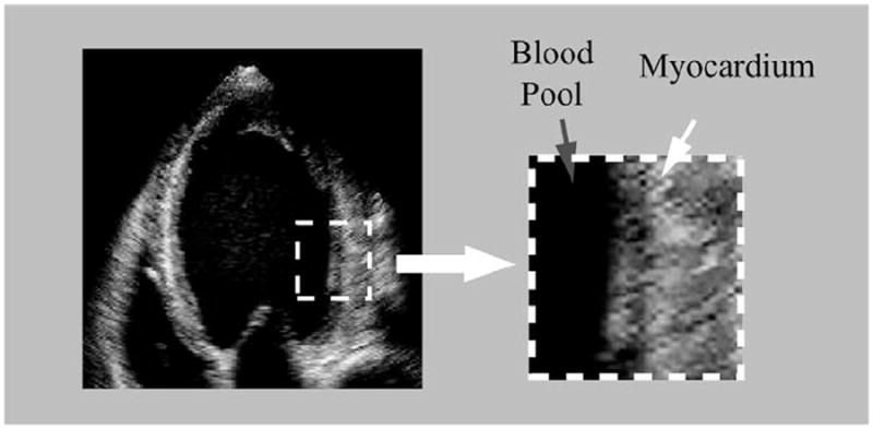
Left ventricular (LV) myocardium has more speckles than the blood pool.

Second, the myocardium/background contrast is lower than the myocardium/blood pool contrast. This is because the myocardium and its adjacent tissues (such as liver) have similar echogenicities, and therefore yield very similar intensity values in ultrasound images. It makes the inferior and lateral sectors of the epicardial (EPI) boundary very ambiguous, as shown in Fig. 2a.

Fig. 2.

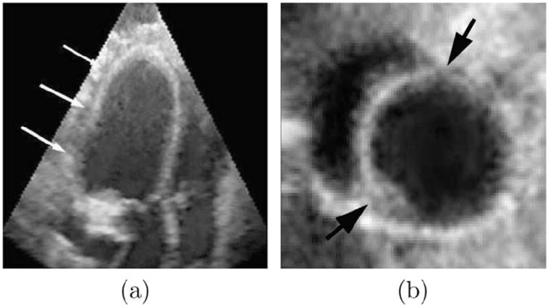
(a) The low myocardium/background contrast makes epicardial (EPI) contour ambiguous, while the endocardial (ENDO) contour is still clear. (b) It is hard to separate left ventricular (LV) myocardium from right ventricular (RV) myocardium at their junctures.

Third, the left ventricular (LV)/right ventricular (RV) junctures pose additional challenges for epicardial (EPI) segmentation. Since the left ventricular (LV) myocardium and right ventricular (RV) myocardium are similar in appearance, separation of one from the other at the juncture point is difficult, as shown in Fig. 2b.

Less extensive information is available on segmentation of the epicardial (EPI) contour compared to endocardial (ENDO) segmentation. Much of the early work focused on two-dimensional (2-D) epicardial (EPI) segmentation. For example, Jacob et al. presented a Kalman filter-based algorithm to track two-dimensional (2-D) endocardial (ENDO) and epicardial (EPI) borders (Jacob et al., 2002). Malassiotis et al. used a temporal learning–filtering approach to identify the two-dimensional (2-D) epicardial (EPI) boundary from ultrasound imaged (Malassiotis and Strintzis, 1999). Chalana et al. developed a multiple active contour based on the extension of two-dimensional (2-D) active contour model to find endocardial (ENDO) and epicardial (EPI) boundaries from a sequence of ultrasound images (Chalana et al., 1996). Setarehdan et al. developed a fuzzy edge detection method to detect and track two-dimensional (2-D) endocardial (ENDO) and epicardial (EPI) contours from a sequence of short-axis echocardiographic data (Setarehdan and Soraghan, 1999).

As three-dimensional (3-D) echocardiography becomes more available, some recent efforts have now been directed towards investigating techniques for three-dimensional (3-D) epicardial (EPI) segmentation. Song et al. treated the segmentation problem as a three-dimensional (3-D) surface fitting problem based on the integration of both low-level image information and a high-level shape prior, through a pixel class prediction mechanism (Song et al., 2002). Yan et al. proposed a multilevel free-form deformation (FFD), driven by fuzzy feature information, to segment the three-dimensional (3-D) endocardial (ENDO) and epicardial (EPI) contours (Yan et al., 2007). Myronenko et al. combined image textual and gradient information to detect endocardial (ENDO) and epicardial (EPI) contours from real-time 3-D (RT3D) echocardiography (Myronenko et al., 2007).

Most of the above methods do not explicitly use constraints due to the spatial relationship between the endocardial (ENDO) and epicardial (EPI) contours, and therefore are limited for the purpose of myocardial segmentation. However, some effort has been made in this direction. Lynch et al. proposed a coupled deformable model with a wall thickness constraint to simultaneously segment the endocardial (ENDO) and epicardial (EPI) contours from cardiac magnetic resonance (MR) images (Lynch et al., 2006). In this approach, the authors assumed that the distance between the endocardial (ENDO) and epicardial (EPI) surfaces were nearly constant throughout the heart cycle, and took this important constraint into consideration in the segmentation process.

This paper is an extended version of our two conference papers (Zhu et al., 2007a,b). It presents an alternative coupled deformable model for tracking and segmentation of left ventricular (LV) myocardial borders from real-time 3-D (RT3D) echocardiographic images. Rather than imposing a constraint on the myocardial wall thickness, we instead assume that the myocardial volume (MV) is nearly constant during a cardiac cycle. This incompressibility constraint is incorporated into the segmentation process in a probabilistic framework, which maximizes the regional inhomogeneities of a cardiac image, while maintaining myocardial volume (MV) during the cycle. By simultaneously evolving the endocardial (ENDO) and epicardial (EPI) surfaces, we are thus able to achieve an automatic segmentation of the full myocardium and concomitantly obtain a representation of the endocardial (ENDO) and epicardial (EPI) surfaces from the cardiac image.

This paper is organized as follows. In Section 2, we discuss the speckle statistics for ultrasound images. In Section 3, we describe the incompressibility property of the myocardium. The speckle statistics discussed in Section 2 and the incompressibility constraint discussed in Section 3 are then incorporated in a maximum a posteriori (MAP) framework presented in Section 4. In Section 5, we discuss the implementation of this framework. Section 6 is the experimental setup and Section 7 shows qualitative and quantitative experimental results on both synthetic and real data. Section 8 provides a discussion of the proposed method, and Section 9 is the conclusion.

2. Statistical modeling of ultrasound speckle

Ultrasound imaging involves receiving acoustic pulse reflected off a scatter medium. The received signal is the sum of signals received from a large number of scattering points located within a resolution cell, giving rise to the speckle pattern. These scatters are randomly or coherently distributed in the tissue, so the speckle has a statistical nature.

Speckle statistics can be initially classified as pre-Rayleigh, Rayleigh, and post-Rayleigh, depending on the density and spatial distribution of the scatter (Shankar, 2000). The simplest model assumes a large number of randomly located scatters and treats the backscattered echo as a random walk. Under these conditions, the echo envelope has a Rayleigh distribution (Wagner et al., 1983), a pattern which is normally referred to as “fully developed” speckle. However, Rayleigh distribution is not necessarily the norm in ultrasound imaging. First, when the number of scatters is not large enough, the envelope statistics are pre-Rayleigh. Second, the scatters may not be randomly located, that is, there may be periodicity in the spatial distribution of scatters, giving rise to post-Rayleigh statistics.

To model the pre-Rayleigh condition, the K-distribution (Jakeman, 1999) has been proposed to account for the low effective scatter density. The K-distribution has two parameters, namely the effective number of scatters and the scaling parameter. These two parameters provide information about the density of scatters, the variation in the scattering amplitude within the resolution cell, and the mean scattering amplitude. To model the post-Rayleigh condition, the Rice distribution (Wagner et al., 1983) has been used to account for a coherent component due to the presence of a regular structure of scatters. Some even more complicated distributions were proposed to handle both pre-Rayleigh and post-Rayleigh distributions, such as generalized K-distribution (Jakeman, 1999) and homodyned K-distribution (Dutt and Greenleaf, 1994).

Unfortunately, the computational complexity of these models is significant (Shankar, 2000), making them inappropriate for segmentation purposes. To address this issue, Shankar et al. proposed modeling speckles using the Nakagami distribution (Shankar, 2000). There are two advantages of the Nakagami distribution. First, it is a general model that can collectively represent the pre-Rayleigh, Rayleigh, and post-Rayleigh conditions that exist in ultrasound images. Second, it is a two-parameter distribution with analytical simplicity. These advantages make the Nakagami distribution useful in ultrasound segmentation. For example, Davignon et al. incorporated the Nakagami distribution in the segmentation process, and formulated the segmentation problem in a multi-resolution Markov random field framework (Davignon et al., 2005).

In (Shankar, 2000), the probability density function (pdf) of the Nakagami distribution is given as:

$$P(x)=\frac{2{\mu }^{\mu }{x}^{2\mu -1}}{\Gamma (\mu ){\omega }^{\mu }}\exp (-\frac{\mu }{\omega }{x}^2)$$ (1)

where μ is a shape parameter conveying information about the envelope statistics, ω is a scaling parameter, and Γ(·) is a Gamma function. Eq. (1) models pre-Rayleigh statistics when μ < 1, post-Rayleigh statistics when μ > 1, and reduces to Rayleigh statistics when μ = 1. Thus, the Nakagami distribution is inclusive of all three cases by appropriate choices of parameter μ.

In Shankar (2000), provides an efficient approach for estimating the shape parameter μ and scaling factor ω, as follows:

$$\mu =\frac{E^2(x^2)}{\mathrm{var}(x^2)}$$ (2)

and

$$\omega =E(x^2)$$ (3)

In this work, we fit the histograms of the blood pool and the myocardium with four distributions (Rayleigh, K, Rice, and Nakagami). Fig. 3 shows two example histograms with fitted distributions, which correspond to the blood pool and myocardium, respectively.

Fig. 3.

The example histograms with fitted distributions. (a) Blood pool, (b) myocardium. Green: Rayleigh, blue: K, red: Rician, black: Nakagami. (For interpretation of the references to colour in this figure legend, the reader is referred to the web version of this article.)

To further quantitatively compare how well the histograms fit the different distribution families, we performed a Pearson chi-squared goodness-of-fit test (see Appendix A). Table 1 shows the average significance values of fit for the blood pool and the myocardium. For the blood pool, the scattering mainly arises from the red blood cells (Angelsen, 1980), which normally have the shape of biconcave disc with a diameter of 8 μm, a maximum thickness of 2.8 μm, and an average volume of 90 μm (Shung and Thieme, 1992). The ultrasound wavelength at 3.5 MHz was 440 μm, which is much larger than the size of the red blood cells. Unlike the blood pool, which has randomly distributed scatters, the myocardium consists of predominantly cardiac muscle fibers, blood vessels, and bile ducts (Shung and Thieme, 1992). The myocardial fibers are more or less cylindrical in shape with a diameter between 10 μm and 20 μm, and occupy approximately 90% volume of the myocardium. As the Nakagami distribution can collectively model pre-Rayleigh, Rayleigh, and post-Rayleigh situations, it has a significance value similar to the K-distribution in the blood pool, and to the Rice distribution in the myocardium. In this paper, we chose the Nakagami distribution to model the intensity of the blood pool and the myocardium.

Table 1.

The significance values of model fits for blood pool and myocardium.

	Rayleigh	K	Rice	Nakagami
Blood pool	0.12	0.59	0.13	0.60
Myocardium	0.15	0.20	0.45	0.57

3. Incompressibility of the Myocardium

The heart is a remarkably efficient and durable mechanical pump composed of complex biological materials. The main structural elements of the myocardium are inter-connected networks of muscle fibers and collagen fibers, as well as matrix that embeds them. The fibers are generally tangential to the endocardial (ENDO) and epicardial (EPI) surfaces, following a path that has a right-handed helical geometry. The interstitial fluid carries only hydrostatic pressure, which, in turn, is affected by the length and configuration changes of the fibers. These cause pressure gradients, which may result in a flow of the matrix. However, since the permeability of the myocardium is low, the fluid flow within the tissue is negligible for the duration of a cardiac cycle. Consequently, the myocardium can be assumed to be nearly incompressible (Glass et al., 1990).

A few independent studies have quantitatively evaluated the changes in myocardial volume (MV) over an entire cardiac cycle. For example, Hamilton et al. performed experiments on frogs, turtles, and dogs (Hamilton and Rompf, 1932). They found the total myocardial volume (MV) to be relatively constant during a cardiac cycle. Hoffman et al. used Dynamic Spatial Reconstructor (DSR) to study the change of myocardial volume (MV) in dogs, and obtained a relatively constant volume that was consistent with Hamilton’s findings (Hoffman and Ritman, 1987, 1985). Bowman et al. using high-resolution magnetic resonance (MR) imaging found a variation of around 5% between end-diastole (ED) and end-systole (ES) (Bowman and Kovacs, 2003). O’Donnell also analyzed the myocardial volume (MV) using magnetic resonance (MR) imaging, and found a difference of about 2.5% between end-diastole (ED) and end-systole (ES) (O’Donnell and Funka-Lea, 1998). The common conclusion of these studies is that the myocardial volume (MV) is nearly constant and its variation is less than 5% during a cardiac cycle. The incompressibility property of the myocardium is used as an important constraint that is taken into account in our approach, as will be detailed in Section 4.3.

4. Cardiac segmentation

4.1. General framework

In Section 2, we discuss the statistical modeling of ultrasound speckle. In Section 3, we describe the incompressibility property of the myocardium. Here, we propose a maximum a posteriori (MAP) framework for segmenting real-time 3-D (RT3D) echocardiographic images by combining image information with a incompressibility constraint.

Let I be a volumetric cardiac image, ϕ_in be the level set representation of the endocardial (ENDO) surface, and ϕ_out be the level set representation of the epicardial (EPI) surface. The maximum a posteriori (MAP) framework that realizes coupled segmentation of the endocardial (ENDO) and epicardial (EPI) surfaces with the incompressibility constraint can be expressed as:

$$\begin{array}{l}({\widehat{\varphi }}_{\mathrm{in}},{\widehat{\varphi }}_{\mathrm{out}})=\arg {\max }_{{\varphi }_{\mathrm{in}},{\varphi }_{\mathrm{out}}}P({\varphi }_{\mathrm{in}},{\varphi }_{\mathrm{out}}\mid I)\\ =\arg {\max }_{{\varphi }_{\mathrm{in}},{\varphi }_{\mathrm{out}}}P(I\mid {\varphi }_{\mathrm{in}},{\varphi }_{\mathrm{out}})p({\varphi }_{\mathrm{in}},{\varphi }_{\mathrm{out}})\\ =\arg {\max }_{{\varphi }_{\mathrm{in}},{\varphi }_{\mathrm{out}}}\left\{\underset{\mathrm{data\; adherence}}{\underbrace{\log P(I\mid {\varphi }_{\mathrm{in}},{\varphi }_{\mathrm{out}})}}+\underset{\mathrm{incompressibility\; constraint}}{\underbrace{\log p({\varphi }_{\mathrm{in}},{\varphi }_{\mathrm{out}})}}\right\}\end{array}$$ (4)

Eq. (4) can be interpreted as a probability function that adheres to image data, modulated by the prior knowledge of the near incompressibility property of the myocardium. In this work, we define the incompressibility constraint within a probabilistic framework, although it is also possible to define it in a deterministic framework (Bistoquet et al., 2008; Saddi et al., 2007; Mansi et al., 2009).

4.2. Data adherence

In echocardiography, the strength of the signal due to the myocardial boundaries depends on the relative orientation of the border to transducer direction. For this reason, conventional intensity gradient-based methods have limited success in ultrasound image segmentation. Region-based methods, however, have been successfully applied to segment images with weak edges (Sarti et al., 2005). In this paper, we develop a region-based deformable model based on the speckle statistics of ultrasound images.

Suppose the entire image is partitioned by the endocardial (ENDO) and epicardial (EPI) surfaces into three regions: left ventricular (LV) blood pool, left ventricular (LV) myocardium, and background (see Fig. 4). The left ventricular (LV) blood pool and the myocardium are homogeneous, and therefore can be modeled with a single probability density function (pdf). In this paper, we use the Nakagami distribution as a probability density function (pdf) for speckles.

$$\begin{array}{l}{p}_1(I)=\frac{2{\mu }_1^{{\mu }_1}{I}^{2{\mu }_1-1}}{\Gamma ({\mu }_1){\omega }_1^{{\mu }_1}}\exp \left(-\frac{{\mu }_1}{{\omega }_1}{I}^2\right)\left(\begin{array}{c}\mathrm{LV}\\ \mathrm{Blood\; Pool}\end{array}\right)\\ p_2(I)=\frac{2{\mu }_2^{{\mu }_2}{I}^{2{\mu }_2-1}}{\Gamma ({\mu }_2){\omega }_2^{{\mu }_2}}\exp \left(-\frac{{\mu }_2}{{\omega }_2}{I}^2\right)\left(\begin{array}{c}\mathrm{LV}\\ \mathrm{Myocardium}\end{array}\right)\end{array}$$

While the histograms of speckle in the blood pool and the myocardium are unimodal, the histogram of the background is not. It is so because the background includes more than one tissue type (e.g. right ventricular (RV) blood pool, right ventricular (RV) myocardium, and other tissues) (as shown in Fig. 4), and therefore modeling it with a single distribution would be insufficient because it contains a wide range of intensity. To circumvent this problem, we use a mixture model to fit the background histogram.

Fig. 4.

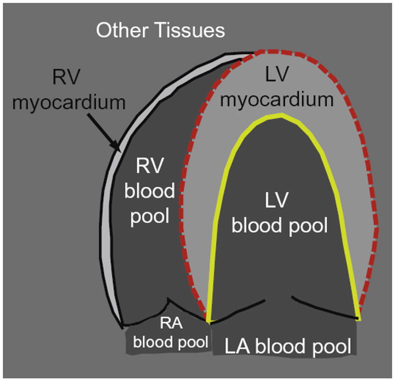
The entire image is partitioned by the endocardial (ENDO) (yellow solid line) and epicardial (EPI) (red dashed line) contours into left ventricular (LV) blood pool, left ventricular (LV) myocardium, and background (outside the dashed red line). While left ventricular (LV) blood pool and myocardium are homogeneous, the background is inhomogeneous because it includes right ventricular (RV) blood pool, right ventricular (RV) myocardium, and other tissues. (For interpretation of the references to colour in this figure legend, the reader is referred to the web version of this article.)

Under the mixture model, the background intensity distribution is given as

$$P_3(I)=\sum _{k=1}^M{\alpha }_k{P}_{3,k}(I;{\mu }_{3,k},{\omega }_{3,k})$$

where M is the number of components, α_k is the mixture proportion of component k that satisfies ${\sum }_{k=1}^M{\alpha }_k=1$, P_3,k(I; μ_3,k, ω_3,k) is the component Nakagami distribution, and μ_3,k and ω_3,k are its shape and scaling parameters. In this paper, we use M = 2 because there are two peaks in the histograms of the background (see Fig. 6c). While the first peak corresponds to the right ventricular (RV) blood pool, the second corresponds to the right ventricular (RV) myocardium and liver.

Fig. 6.

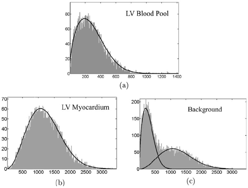
The histograms of left ventricular (LV) blood pool, left ventricular (LV) myocardium, and background from one example cardiac image with estimated intensity distributions superimposed on them. (a) μ₁ = 0.71 and ω₁ = 1.24 × 10⁵; (b) μ₂ = 1.47 and ω₂ = 1.32 × 10⁶; (c) α₁ = 0.42, α₂ = 0.58, μ_3,1 = 0.75, μ_3,2 = 1.43, ω_3,1 = 1.11 × 10⁵, and ω_3,2 = 1.29 × 10⁶.

Let Ω₁ = {x∣ϕ_in(x) ≤ 0} be the left ventricular (LV) blood pool, Ω₂ = {x∣ϕ_in(x) > 0 and ϕ_out (x) ≤ 0} be the left ventricular (LV) myocardium, and Ω₃ = {x∣ϕ_out(x) > 0} be the background.

Thus, the data adherence term can be defined as

$$\log P(I\mid {\varphi }_{\mathrm{in}},{\varphi }_{\mathrm{out}})=\sum _{l=1}^3{\mathit{\int }}_{{\Omega }_l}\log P_l(I)d\mathbf{x}$$ (5)

The maximization of Eq. (5) can be interpreted as the propagation of ϕ_in and ϕ_out that maximizes the piecewise homogeneities of three regions.

4.3. Incompressibility constraint

As explained in Section 3, the myocardium is nearly incompressible and the myocardial volume (MV) changes less than 5% during a cardiac cycle. Thus, the myocardial volume (MV) at a particular frame can be modeled by a Gaussian distribution N(V₀, ${\sigma }_0^2$)

$$P({\varphi }_{\mathrm{in}},{\varphi }_{\mathrm{out}})=\frac{1}{\sqrt{2\pi }{\sigma }_0}\exp \left\{-\frac{{(V-V_0)}^2}{2{\sigma }_0^2}\right\}$$ (6)

where V = ∫_Ω2 dx is the myocardial volume (MV). By invoking the three-sigma rule,¹ we have the following relationship

$$\begin{array}{l}3{\sigma }_0=0.025V_0\\ {\sigma }_0=\frac{1}{120}{V}_0\end{array}$$

Eq. (6) defines a probability function that favors consistent myocardial volume (MV) during a cardiac cycle, while allowing a small variation of around 5%.

4.4. Optimization

Combining Eqs. (4)-(6), the maximization of posterior likelihood is equivalent to the maximization of the following equation

$$\begin{array}{lll}({\widehat{\varphi }}_{\mathrm{in}},{\widehat{\varphi }}_{\mathrm{out}})& =& \arg {\max }_{{\varphi }_{\mathrm{in}},{\varphi }_{\mathrm{out}}}\{\log P(I\mid {\varphi }_{\mathrm{in}},{\varphi }_{\mathrm{out}})+\log P({\varphi }_{\mathrm{in}},{\varphi }_{\mathrm{out}})\}\\ & =& \arg {\max }_{{\varphi }_{\mathrm{in}},{\varphi }_{\mathrm{out}}}\left\{\sum _{l=1}^3{\mathit{\int }}_{{\Omega }_l}\log P_l(I)d\mathbf{x}-\frac{{(V-V_0)}^2}{2{\sigma }_0^2}\right\}\end{array}$$ (7)

To deform ϕ_in towards the optimal solution, we define a thin-plate spline (TPS) warp L(·; Θ_in) (see Appendix B for an overview) that deforms a fixed level set template ${\varphi }_{\mathrm{in}}^0$ to ϕ_in (Taron et al., 2007), i.e.

$${\varphi }_{\mathrm{in}}(\mathbf{x})={\varphi }_{\mathrm{in}}^0(L(\mathbf{x};{\Theta }_{\mathrm{in}}))$$

Thus, the deformation of ϕ_in depends on the thin-plate spline (TPS) warping, which is determined by the control points Θ_in. In other words, we define the segmentation problem as one that finds an optimal thin-plate spline (TPS) warping that maximizes Eq. (7). Similarly, we define ${\varphi }_{\mathrm{out}}(\mathbf{x})={\varphi }_{\mathrm{out}}^0(L(\mathbf{x};{\Theta }_{\mathrm{out}}))$.

By taking the gradients with respect to Θ_in and Θ_out (see C for details), we have

$$\frac{\partial {\Theta }_{\mathrm{in}}}{\partial \tau }={\mathit{\int }}_{\partial C_{12}}\left(\log \frac{P_1}{P_2}+\frac{V-V_0}{{\sigma }_0^2}\right)\nabla {\varphi }_{\mathrm{in}}({\mathbf{x}}^{\prime })\frac{\partial L}{\partial {\Theta }_{\mathrm{in}}}(\mathbf{x};{\Theta }_{\mathrm{in}})d\mathbf{x}$$ (8)

$$\frac{\partial {\Theta }_{\mathrm{out}}}{\partial \tau }={\mathit{\int }}_{\partial C_{23}}\left(\log \frac{P_2}{P_3}-\frac{V-V_0}{{\sigma }_0^2}\right)\nabla {\varphi }_{\mathrm{out}}({\mathbf{x}}^{\prime })\frac{\partial L}{\partial {\Theta }_{\mathrm{out}}}(\mathbf{x};{\Theta }_{\mathrm{out}})d\mathbf{x}$$ (9)

where ∂C₁₂ is the interface between Ω₁ and Ω₂, i.e. the endocardial (ENDO) surface, while ∂ C₂₃ is the interface between Ω₂ and Ω₃, i.e. the epicardial (EPI) surface. ∇ϕ_in(x′) and ∇ϕ_out(x′) are the gradients evaluated at the transformed position x′ = L(x; Θ). $\frac{\partial L}{\partial {\Theta }_{\mathrm{in}}}(\mathbf{x};{\Theta }_{\mathrm{in}})$ is the gradient of thin-plate spline (TPS) warping with respect to Θ_in, and $\frac{\partial L}{\partial {\Theta }_{\mathrm{out}}}(\mathbf{x};{\Theta }_{\mathrm{out}})$ is the gradient of thin-plate spline (TPS) warping with respect to Θ_out.

5. Implementation

In this section, we detail the implementation of the segmentation approach described in Section 4. Our method is a sequential segmentation approach that starts with a manual segmentation of the first frame, and then uses the final segmentation of the previous frame to initialize the current frame. We also use the segmented image from the previous frame to estimate the intensity distribution parameters for the current frame. The estimated parameters are fed into the data adherence term which, in combination with the incompressibility constraint, propagates the endocardial (ENDO) and epicardial (EPI) surfaces. The flowchart of our segmentation approach is illustrated in Fig. 5.

Fig. 5.

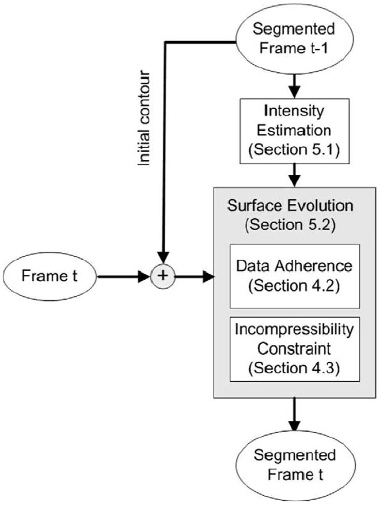
Flowchart of our segmentation method.

5.1. Intensity estimation

In Section 4.2, we model the left ventricular (LV) blood pool and myocardium with the Nakagami distribution, and background with a mixture of Nakagami distribution. While it is possible to estimate intensity-distribution parameters in parallel with surface evolution for each iteration, we approximate these parameters from the segmented image of the previous frame. By doing this, we implicitly assume that the intensity distribution from two adjacent frames are similar. This is valid because (1) the inter-frame motion is not significant (although the cumulative motion from end-diastole (ED) to end-systole (ES) is large), and (2) histogram is a global measure that is insensitive to small inter-frame changes.

First, we use Eqs. (2) and (3) to estimate the parameters for the left ventricular (LV) blood pool (μ₁ and ω₁) and for the left ventricular (LV) myocardium (μ₂ and ω₂).

Second, we describe how to estimate the parameters for the background. In Section 4.2, we use a mixture model to fit the background histogram, and an Expectation–Maximization (EM) algorithm to estimate the parameters for the mixture model (α₁, α₂, μ_3,1, μ_3,2, ω_3,1, and ω_3,2).

Suppose we represent the voxels in the background as a vector {I₁,…,I_N}, where N is the number of voxels in the background. The Expectation–Maximization (EM) algorithm considers {I₁,…,I_N} as observations, and augments each I_i with a set of labels {z_ik} (1 ≤ k ≤ M), where M is the number of components in the mixture model. We define z_ik = 1 if observation I_i comes from the kth mixture component, and z_ik = 0 if I_i does not come from the k component.

Given an initial estimate, the Expectation–Maximization (EM) algorithm iterates an expectation step (E-step) and maximization step (M-step) until convergence (see Appendix D for derivation).

1. E-step Compute the posterior probability of the ith observation coming from the kth mixture component:

   $$z_{\mathit{ik}}^{(n)}=P(z_{\mathit{ik}}=1\mid I_i,{\alpha }_k^{(n)},{\mu }_{3,k}^{(n)},{\omega }_{3,k}^{(n)})=\frac{{\alpha }_k^{(n)}{p}_{3,k}(I_i;{\mu }_{3,k}^{(n)},{\omega }_{3,k}^{(n)})}{\sum _k{\alpha }_k^{(n)}{P}_{3,k}(I_i;{\mu }_{3,k}^{(n)},{\omega }_{3,k}^{(n)})}$$
2. M-step Update the estimate of parameters (α_k, μ_3,k, and ω_3,k) of the mixture component:

   $$\begin{array}{lll}{\omega }_{3,k}^{(n+1)}& =& \frac{\sum _i{z}_{\mathit{ik}}^{(n)}{I}_i^2}{\sum _i{z}_{\mathit{ik}}^{(n)}}\\ {\mu }_{3,k}^{(n+1)}& =& \frac{3-s+\sqrt{{(s-3)}^2+24s}}{12s}\end{array}$$

   where

   $$\begin{array}{l}s=\frac{{\sum }_i{z}_{\mathit{ik}}^{(n)}\left(\log {\omega }_{3,k}^{(n+1)}-2\log I_i+I_i^2/{\omega }_{3,k}^{(n+1)}-1\right)}{{\sum }_i{z}_{\mathit{ik}}^{(n)}}\\ {\alpha }_k^{(n+1)}=\frac{{\sum }_i{z}_{\mathit{ik}}^{(n)}}{N}\end{array}$$
3. If converged, then stop. Otherwise, repeat step 1. In this work, the following criterion is considered the indicator of convergence:

   $$\max \left\{\sum _{k=1}^M\left|{\alpha }_k^{(n+1)}-{\alpha }_k^{(n)}\right|,\sum _{k=1}^M\left|{\omega }_{3,k}^{(n+1)}-{\omega }_{3,k}^{(n)}\right|,\sum _{k=1}^M\left|{\mu }_{3,k}^{(n+1)}-{\mu }_{3,k}^{(n)}\right|\right\}<{10}^{-6}$$

The initial estimate of the Expectation–Maximization (EM) algorithm is chosen as follows:

• For the first frame, we set ${\mu }_{3,1}^{(0)}={\mu }_1$ and ${\omega }_{3,1}^{(0)}={\omega }_1$. This is because the first component of the mixture model, which corresponds to the right ventricular (RV) blood pool and lung air, has similar echogenicities to the left ventricular (LV) blood pool. Similarly, we set ${\mu }_{3,2}^{(0)}={\mu }_2$ and ${\omega }_{3,2}^{(0)}={\omega }_2$ because the second component of the mixture model, which corresponds to the right ventricular (RV) myocardium and liver, has similar echogenicities to the left ventricular (LV) myocardium. We also found by experiment that ${\alpha }_1^{(0)}=0.5$ and ${\alpha }_2^{(0)}=0.5$ were appropriate for most of the data sets. In practice, it required about 10 iterations before convergence.

• For the subsequent frames, we initialized the Expectation–Maximization (EM) algorithm with the estimated parameters from the previous frame. In practice, it required less than 5 iterations before convergence.

In Fig. 6, we show the histograms of three regions from one example image with fitted intensity distribution functions.

5.2. Surface evolution

As explained in Section 4.4, the endocardial (ENDO) and epicardial (EPI) surfaces are propagated by updating the thin-plate spline (TPS) control points Θ_in and Θ_out. From a computational point of view, a small set of control points is desired to reduce the computational load. However, a small set of points may fail to capture some local shape features. In this work, we iso-sampled around 150 control points on the endocardial (ENDO) surface and 135 control points on the epicardial (EPI) surface, as shown in Fig. 7. We placed more control points on the endocardial (ENDO) surface than on the epicardial (EPI) surface because the endocardial (ENDO) surface was more curved (e.g. due to papillary muscles) than the epicardial (EPI) surface.

Fig. 7.

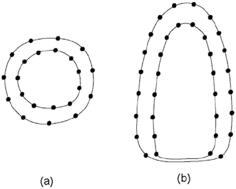
Distribution of control points. (a) Short-axis, (b) long-axis.

Starting from the final segmentation of the previous frame, we propagated the endocardial (ENDO) and epicardial (EPI) surfaces by iterating the following three steps.

1. Let n be the number of iterations, update ${\Theta }_{\mathrm{in}}^{(n+1)}$ and ${\Theta }_{\mathrm{out}}^{(n+1)}$ as in follows:

   $$\begin{array}{lll}{\Theta }_{\mathrm{in}}^{(n+1)}& =& {\Theta }_{\mathrm{in}}^{(n)}+\tau {\mathit{\int }}_{\partial C_{12}}\left(\log \frac{P_1}{P_2}+\frac{V-V_0}{{\sigma }_0^2}\right)\nabla {\varphi }_{\mathrm{in}}^{(n)}({\mathbf{x}}^{\prime })\\ & & \times \frac{\partial L}{\partial {\Theta }_{\mathrm{in}}}\left(\mathbf{x};{\Theta }_{\mathrm{in}}^{(n)}\right)d\mathbf{x}\end{array}$$ (10)

   $$\begin{array}{lll}{\Theta }_{\mathrm{out}}^{(n+1)}& =& {\Theta }_{\mathrm{out}}^{(n)}+\tau {\mathit{\int }}_{\partial C_{23}}\left(\log \frac{P_2}{P_3}-\frac{V-V_0}{{\sigma }_0^2}\right)\nabla {\varphi }_{\mathrm{out}}^{(n)}({\mathbf{x}}^{\prime })\\ & & \times \frac{\partial L}{\partial {\Theta }_{\mathrm{out}}}\left(\mathbf{x};{\Theta }_{\mathrm{in}}^{(n)}\right)d\mathbf{x}\end{array}$$ (11)

   where τ is the numerical time step. In practice, we chose τ = 2.5 × 10⁻⁶. It should be noted that the domains of integration in Eqs. (10) and (11) are the endocardial (ENDO) and epicardial (EPI) surfaces, respectively. Therefore, there is no need to parse the entire image at every iteration.

2. Update the thin-plate spline (TPS) warping $L(\mathbf{x};{\Theta }_{\mathrm{in}}^{(n+1)})$ and $L(\mathbf{x};{\Theta }_{\mathrm{out}}^{(n+1)})$ with ${\Theta }_{\mathrm{in}}^{(n+1)}$ and ${\Theta }_{\mathrm{out}}^{(n+1)}$ obtained in step 1. As explained in Appendix B, we used a regularization parameter λ to control the stiffness of the transform. In practice, we used a stiff-to-flexible strategy to regularize the thin-plate spline (TPS) warping, as described in Appendix B. Specifically, we started with λ^initial = 3, and gradually decreased it by a scaling factor γ = 2 for the endocardial (ENDO) contour and γ = 1.2 for the epicardial (EPI) contour in each iteration until convergence. We used a larger λ for the epicardial (EPI) contour because the epicardial (EPI) did not have as many local shape features as the endocardial (ENDO) contour. Also, for efficiency, we only updated $L(\mathbf{x};{\Theta }_{\mathrm{in}}^{(n+1)})$ within a narrow band around the zero level-set of ${\varphi }_{\mathrm{in}}^{(n)}(\mathbf{x})$, and $L(\mathbf{x};{\Theta }_{\mathrm{out}}^{(n)})$ within a narrow band around the zero level-set of ${\varphi }_{\mathrm{out}}^{(n)}(\mathbf{x})$. In practice, we chose the width of the narrow band as 2 mm.

3. Update the endocardial (ENDO) and epicardial (EPI) level-set functions ${\varphi }_{\mathrm{in}}^{(n+1)}(\mathbf{x})={\varphi }_{\mathrm{in}}^0\left(L\right(\mathbf{x};{\Theta }_{\mathrm{in}}^{(n+1)}\left)\right)$ and ${\varphi }_{\mathrm{out}}^{(n+1)}(\mathbf{x})={\varphi }_{\mathrm{out}}^0\left(L\right(\mathbf{x};{\Theta }_{\mathrm{out}}^{(n+1)}\left)\right)$ in their narrow bands.

The final endocardial (ENDO) and epicardial (EPI) surfaces can be extracted from their corresponding level set functions, respectively. As the inter-frame motion (the motion between two adjacent frames) is small, we normally need 5–10 iterations before convergence.

6. Experimental setup

6.1. Data acquisition

We performed experiments on both synthetic and real echocardiographic data.

6.1.1. Synthetic data

The benefits of using synthetic data are the availability of ground truth segmentation and controllable image quality. In our experiments, we generated synthetic data using the Field II ultrasound system simulation program (Jensen and Svendsen, 1992; Jensen, 1996). This simulation program includes methods for implementing different array and transducer geometries with apodization, beamforming, absorption effects, and the ability to create synthetic phantoms made from an organized set of point scatters. The imaging parameters in our experiments were as follows: probe center frequency = 5 MHz, probe matrix dimensions = 64 × 32, element width = 0.154 mm, element height = 0.154 mm, focus depth = 70 mm, sampling frequency = 100 MHz, number of scanlines = 40 × 40. We used manual segmentation from cardiac magnetic resonance (MR) images to generate three-dimensional (3-D) synthetic phantoms by randomly distributing 2 × 10⁶ scatters within each three-dimensional (3-D) phantom. The Field II program computed the radio-frequency (RF) signal for different imaging directions, and stored each radio-frequency (RF) line in a separate file. These files were then used to assemble an ultrasound image. We generated a total of five synthetic sequences, each consisting of 16 temporal frames. The results from the automatic method were compared to the ground truth segmentation that was used to generate the synthetic images.

6.1.2. Real data

The real data were acquired using a Philips IE33 echocardiographic system with a 4MHz X4 xMatrix transducer. This transducer consists of 3000 miniaturized piezoelectric elements and offers steering in both azimuth and elevation of the beam, permitting real-time volumetric image acquisition and rendering (Philips, 2005). While most commercial systems only provide post-processed B-mode images, the statistical properties of which are hard to model due to incomplete knowledge of the post-processing inside the machine (Tao et al., 2006), the IE33 system allows direct access to the unprocessed radio-frequency (RF) signals through a radio-frequency (RF) signal capture board connected to a personal computer. This computer then performs radio-frequency (RF) signal filtering and demodulation using a computer program, obtaining the envelope of the radio-frequency (RF) signal and using it as input in our approach.

In our work, we acquired in total of 11 sequences of canine real-time 3-D (RT3D) echocardiographic images, including five normal and six post-infarcted sequences. Each sequence consisted of 20–30 frames per cardiac cycle depending on the cardiac rate. Therefore, we ran our program with a total of 286 sets of volumetric data. Considering inter-observer variability, we asked three experts, blind to each other, to independently outline the endocardial (ENDO) and epicardial (EPI) contours of all frames using the “4-D Surface Editor” of the Bioimage Suite software (Papademetris et al., 2006).

6.2. Comparison with other approaches

In this work, we compared the results from our approach with those from two other closely related algorithms. The first of these is the unconstrained version of our approach. This algorithm has the same data adherence term as our approach and uses the same thin-plate spline (TPS) level-set (i.e. the same number of landmarks and regularization parameter), but it lacks the incompressibility constraint. The second algorithm is an alternative coupled deformable model that features a wall thickness constraint (Lynch et al., 2006). This coupled deformable model evolved according to (1) image information (gradient and texture), (2) a wall thickness constraint, and (3) a shape prior obtained from a set of training samples. In this work, we used a “leave-one-out” approach to build the shape prior, in order to maximize the effective size of the training set. The wall thickness constraint included two parameters d and w, where parameter d specified the preferred distance between the endocardial (ENDO) and epicardial (EPI) surfaces, while parameter w specified the transition width. The shape prior was weighted by the parameter β. To find an appropriate value for parameter d, we computed the average wall thickness from the ground truth segmentation of five synthetic sequences and from manual segmentation of the 11 canine sequences. In practice, we set d = 7.1 for synthetic data and d = 6.6 for real data. Also, we found by experiment that a large w would cause leakage of the epicardial (EPI) contour. We therefore chose the smallest w that did not have a leakage problem. In practice, we set w = 4.1 for synthetic data and w = 3.6 for real data. We also found by experiment that β = 1 was appropriate for most data sets. These settings were roughly consistent with the ones used in Lynch et al. (2006).

6.3. Quantitative measures

To quantitatively evaluate the segmentation results, we used two distance metrics, namely the mean absolute distance (MAD) and the Hausdorff distance (HD), and one area metric, namely the Dice Similarity Coefficient (DSC).

Let A and B be two surfaces from automatic and manual segmentation, respectively. Suppose they are represented by point sets, i.e. A = {a₁, a₂,…,a_n} and B = {b₁, b₂,…,b_m}, we define

$$\begin{array}{l}\mathrm{MAD}(A,B)=\frac{1}{2}\left\{\frac{1}{n}\sum _{i=1}^{n}d({\mathbf{a}}_i,B)+\frac{1}{m}\sum _{j=1}^{m}d({\mathbf{b}}_j,A)\right\}\\ \mathrm{HD}(A,B)=\max \{{\max }_i\{d({\mathbf{a}}_i,B)\},{\max }_j\{d({\mathbf{b}}_j,A)\}\}\end{array}$$

where d(a_i, B) = min_j∥b_j − a_i∥. While mean absolute distance (MAD) is a global measure of the match between two surfaces, Hausdorff distance (HD) reflects their local similarities.

Let Ω_A and Ω_B be the regions enclosed by surfaces A and B, respectively, the Dice Similarity Coefficient (DSC) is defined as

$$\mathrm{DSC}=\frac{2·\mathrm{Volume}({\Omega }_A\cap {\Omega }_B)}{\mathrm{Volume}({\Omega }_A)+\mathrm{Volume}({\Omega }_B)}$$

7. Experimental results

7.1. Synthetic data

Fig. 8 qualitatively compares the segmentation results using the deformable models with no constraint, with the wall thickness constraint, and with the incompressibility constraint. For the endocardial (ENDO) contours, the results from all three algorithms were similar. However, the epicardial (EPI) contour from the unconstrained deformable model leaked into the background due to the low contrast between the left ventricular (LV) myocardium and the background. The deformable model with the wall thickness constraint outperformed the unconstrained one by preventing the epicardial (EPI) contour from leaking into the background. However, the epicardial (EPI) contour was less accurate in the regions with non-uniform wall thickness, e.g. the regions where the papillary muscles were present, as shown in Fig. 8b. This was more evident in ultrasound images than in magnetic resonance (MR) images because the epicardial (EPI) boundary is fuzzier in ultrasound images and does not provide sufficient image information to pull the endocardial (ENDO) contour to its proper position. When the incompressibility constraint was applied, however, the epicardial (EPI) contour converged to its correct position because the incompressibility constraint imposed a restriction on the myocardial volume (MV) while allowing variations in the myocardial wall thickness.

Fig. 8.

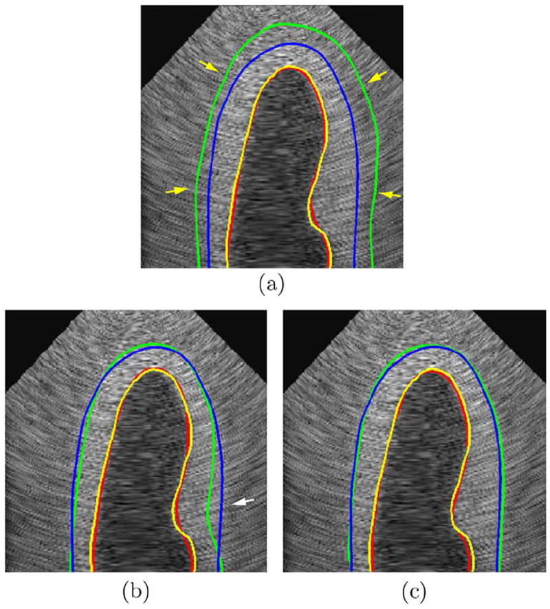
Comparison of results using unconstrained deformable model, the one with the wall thickness constraint, and the one with the incompressibility constraint. (a) without any constraint, (b) with the wall thickness constraint, (c) with the incompressibility constraint. Red line: automatic endocardial (ENDO) contour. Yellow line: ground truth endocardial (ENDO) contour. Green line: automatic epicardial (EPI) contour. Blue line: ground truth epicardial (EPI) contour. Yellow arrow: leakage of the epicardial (EPI) contour. White arrow: d₁ > d₂ in (c) while the wall thickness constraint forced d′₁ to be close to d′₂ in (b). (For interpretation of the references to colour in this figure legend, the reader is referred to the web version of this article.)

Figs. 9 and 10 illustrate the segmentation errors (using mean absolute distance (MAD), Hausdorff distance (HD), and Dice Similarity Coefficient (DSC)) as a function of the cardiac cycle. When the incompressibility constraint was applied, the segmentation accuracy did not change substantially throughout the cycle, although the segmentation errors at the end of the cycle (for endocardial (ENDO) contours, mean absolute distance (MAD) = 1.11 mm, Hausdorff distance (HD) = 2.13, and Dice Similarity Coefficient (DSC) = 96.8%; for epicardial (EPI) contours, mean absolute distance (MAD) = 1.47 mm, Hausdorff distance (HD) = 2.42 mm, and Dice Similarity Coefficient (DSC) = 95.2%) were slightly larger than those at the beginning of the cycle (for endocardial (ENDO) contours, mean absolute distance (MAD) = 0.97 mm, Hausdorff distance (HD) = 1.78 mm, and Dice Similarity Coefficient (DSC) = 97.6%; for epicardial (EPI) contours, mean absolute distance (MAD) = 1.38 mm, Hausdorff distance (HD) = 2.15 mm, Dice Similarity Coefficient (DSC) = 97.1%). This was because we used the final segmentation from the previous frame to estimate the intensity-distribution parameters for the current frame.

Fig. 9.

Segmentation errors of the endocardial (ENDO) contours for synthetic images as functions of time over the cardiac cycle. (a) Mean absolute distance (MAD), (b) Hausdorff distance (HD), (c) Dice Similarity Coefficient (DSC).

Fig. 10.

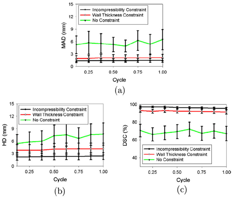
Segmentation errors of the epicardial (EPI) contours for synthetic images as functions of time over the cardiac cycle. (a) Mean absolute distance (MAD), Hausdorff distance (HD), (c) Dice Similarity Coefficient (DSC).

Fig. 9 also shows that the segmentation results for the endocardial (ENDO) contours were similar for all three methods (i.e. with no constraint, with the wall thickness constraint, and with the incompressibility constraint). However, the segmentation results for the epicardial (EPI) contours differed substantially, as shown in Fig. 10. When no constraint was applied, the epicardial (EPI) contours leaked into the background, leading to a global segmentation error. When the wall thickness constraint was applied, the coupling between the endocardial (ENDO) and epicardial (EPI) contours prevented the epicardial (EPI) contour from leaking into the background. The mean absolute distance (MAD) decreased, on average, by 3.66 mm over the cycle, the Hausdorff distance (HD) decreased by 2.56 mm, and the Dice Similarity Coefficient (DSC) increased by 21.46%. The mean absolute distance (MAD) and Dice Similarity Coefficient (DSC) obtained with the incompressibility constraint (mean absolute distance (MAD) = 1.44 mm and Dice Similarity Coefficient (DSC) = 96.34%, on average, over the cycle) were similar to those obtained with the wall thickness constraint (mean absolute distance (MAD) = 2.01 mm and Dice Similarity Coefficient (DSC) = 92.54%, on average, over the cycle), although the results obtained with the incompressibility constraint were slightly better. This implies that the results obtained with the wall thickness constraint were globally correct. However, the Hausdorff distance (HD) obtained with the incompressibility constraint was 1.77 mm smaller than that using the wall thickness constraint, implying that the results obtained with the wall thickness constraint were locally inaccurate.

To further explore the distribution of local segmentation errors, we used a 17-segment model (Cerqueira et al., 2002) dividing the left ventricular (LV) into equal thirds perpendicular to the long-axis of the heart, generating basal, mid-cavity, and apical slices. Then the basal and mid-cavity slices are further divided into six segments of 60° each. Similarly, the apical slices are partitioned into four sectors, i.e. the septal sector and three equal subsectors for the lateral sector. A diagram of the 17-segment model is shown in Fig. 11.

Fig. 11.

The diagram of 17-segment model (Cerqueira et al., 2002).

Table 2 shows the regional mean absolute distance (MAD)s computed on the different sectors of the endocardial (ENDO) surface according to the 17-segment model. No significant differences were observed in the segmentation results obtained with either no constraint, with the wall thickness constraint, or with the incompressibility constraint. This is because the endocardial (ENDO) boundaries are relatively clearer than the epicardial (EPI) boundaries.

Table 2.

Comparison of regional endocardial (ENDO) mean absolute distance (MAD)s on synthetic data (in mm).

		No constraint	Wall thickness constraint	Incompressibility constraint
BA	A	1.08 ± 0.20	1.13 ± 0.21	1.00 ± 0.18
	AL	1.10 ± 0.21	1.19 ± 0.24	1.06 ± 0.23
	IL	1.09 ± 0.23	1.14 ± 0.21	0.99 ± 0.22
	I	1.11 ± 0.24	1.18 ± 0.23	1.09 ± 0.23
	IS	1.07 ± 0.19	1.12 ± 0.19	0.97 ± 0.17
	AS	1.08 ± 0.19	1.13 ± 0.20	0.96 ± 0.18
MC	A	1.09 ± 0.20	1.15 ± 0.24	0.98 ± 0.20
	AL	1.12 ± 0.23	1.25 ± 0.27	1.07 ± 0.22
	IL	1.12 ± 0.21	1.20 ± 0.26	1.03 ± 0.20
	I	1.13 ± 0.22	1.26 ± 0.28	1.04 ± 0.22
	IS	1.07 ± 0.20	1.19 ± 0.23	0.99 ± 0.19
	AS	1.12 ± 0.21	1.15 ± 0.22	1.01 ± 0.20
AP	A	1.11 ± 0.21	1.12 ± 0.21	1.02 ± 0.21
	L	1.12 ± 0.22	1.13 ± 0.22	1.06 ± 0.23
	I	1.10 ± 0.21	1.13 ± 0.23	1.05 ± 0.22
	S	1.12 ± 0.19	1.14 ± 0.23	1.08 ± 0.24

BA: basal, MC: mid-cavity, AP: apical, A: anterior, AL: anterolateral, IL: inferolateral, I: inferior, IS: inferoseptal, AS: anteroseptal, L: lateral, S: septal.

Table 3 shows the regional mean absolute distance (MAD)s computed on the different sectors of the epicardial (EPI) surface according to the 17-segment model. The deformable model with the wall thickness constraint outperformed the unconstrained model by having globally correct segmentation. However, the segmentation results obtained with the wall thickness constraint were less accurate, in comparison with the incompressibility constraint, at the mid-ventricular anterolateral and inferior sectors (mean absolute distance (MAD) = 3.15 mm for the mid-ventricular anter-olateral sector and 3.07 mm for the mid-ventricular inferior sector). This is because the presence of the papillary muscles causes the inhomogeneity of the wall thickness at these sectors. In contrast, when the incompressibility constraint was applied, the mean absolute distance (MAD) decreased by 1.65 mm for the mid-ventricular anterolateral sector and by 1.58 for the mid-ventricular inferior sector.

Table 3.

Comparison of regional epicardial (EPI) mean absolute distance (MAD)s on synthetic data (in mm).

		No constraint	Wall thickness constraint	Inconipressibility constraint
BA	A	5.62 ± 2.34	1.79 ± 0.57	1.39 ± 0.41
	AL	5.72 ± 2.39	1.92 ± 0.62	1.49 ± 0.46
	IL	5.70 ± 2.37	1.77 ± 0.57	1.40 ± 0.42
	I	5.69 ± 2.35	1.93 ± 0.62	1.47 ± 0.44
	IS	5.70 ± 2.38	1.84 ± 0.61	1.45 ± 0.46
	AS	5.65 ± 2.36	1.85 ± 0.60	1.42 ± 0.43
MC	A	5.64 ± 2.38	1.80 ± 0.58	1.38 ± 0.40
	AL	5.71 ± 2.40	3.15 ± 1.02	1.50 ± 0.48
	IL	5.69 ± 2.37	1.90 ± 0.61	1.46 ± 0.45
	I	5.68 ± 2.38	3.07 ± 1.01	1.49 ± 0.47
	IS	5.69 ± 2.39	1.88 ± 0.60	1.40 ± 0.43
	AS	5.66 ± 2.40	1.79 ± 0.56	1.39 ± 0.41
AP	A	5.64 ± 2.37	1.85 ± 0.60	1.43 ± 0.43
	L	5.69 ± 2.40	1.84 ± 0.57	1.45 ± 0.42
	I	5.71 ± 2.40	1.85 ± 0.56	1.44 ± 0.45
	S	5.68 ± 2.39	1.92 ± 0.60	1.43 ± 0.44
APX	APX	5.74 ± 2.36	1.94 ± 0.52	1.46 ± 0.44

BA: basal, MC: mid-cavity, AP: apical, APX: apex A: anterior, AL: anterolateral, IL: inferolateral, I: inferior, IS: inferoseptal, AS: anteroseptal, L: lateral, S: septal.

7.2. Real data

Fig. 12 shows the long-axis view of automatically segmented endocardial (ENDO) and epicardial (EPI) contours at frames 2, 5, 8, 11 during ventricular systole. Fig. 13 shows the corresponding three-dimensional (3-D) endocardial (ENDO) and epicardial (EPI) surfaces.

Fig. 12.

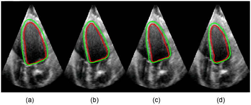
Long axis view of segmented endocardial (ENDO) and epicardial (EPI) contours at frames 2, 5, 8, and 11 during cardiac systole. (a) frame 2, (b) frame 5, (c) frame 8, (d) frame 11.

Fig. 13.

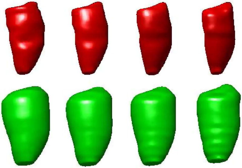
Three-dimensional (3-D) rendering of segmented endocardial (ENDO) and epicardial (EPI) surfaces at frames 2, 5, 8, and 11 during cardiac systole. Upper: endocardial (ENDO), Lower: epicardial (EPI).

Fig. 14 compares the segmentation results obtained with and without the incompressibility constraint. While the endocardial (ENDO) border was correctly detected even without the incompressibility constraint, the epicardial (EPI) contour leaked into other tissues (such as liver) that were similar in appearance to the myocardium. This is because the left ventricular (LV) myocardium/background contrast is lower than the left ventricular (LV) blood pool/myocardium contrast. This low contrast obscures the exact location of the epicardial (EPI) boundary, making epicardial (EPI) segmentation more challenging than endocardial (ENDO) segmentation. When the incompressibility constraint was applied, however, the coupling of the endocardial (ENDO) and epicardial (EPI) contours prevented leaking of the epicardial (EPI) contour.

Fig. 14.

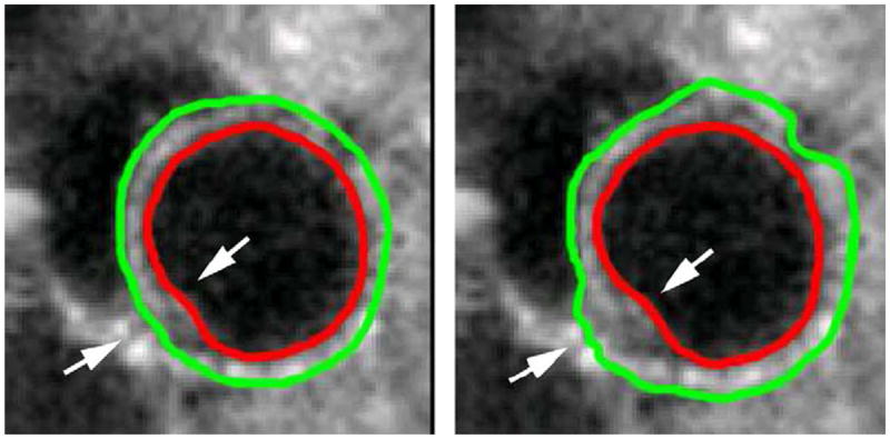
Comparison of epicardial (EPI) segmentation with and without the incompressibility constraint. (a) with the incompressibility constraint; (b) without the incompressibility constraint. Arrow: myocardium juncture.

As explained in Section 1, another challenge in the segmentation of the epicardial (EPI) boundary is the presence of the left ventricular (LV)/right ventricular (RV) myocardium junctures. The intensity similarity between the left ventricular (LV) and right ventricular (RV) myocardium makes the epicardial (EPI) boundary ambiguous at these junctures. When no constraint was applied, the epicardial (EPI) contour evolved out to segment the right ventricular (RV) myocardium. In contrast, when the incompressibility constraint was applied, the left ventricular (LV) myocardium was successfully separated from the right ventricular (RV) myocardium at the junctures, as shown in Fig. 14.

To quantify the segmentation errors, we used manual segmentation as ground truth and compared the automatic contour with the manual contour. As mentioned in Section 6.1, we asked three experts, blind to each other, to trace out the endocardial (ENDO) and epicardial (EPI) contours independently. To take into account inter-observer differences, we computed the mean absolute distance (MAD), Hausdorff distance (HD), and Dice Similarity Coefficient (DSC) for every two manual contours (manual–manual mean absolute distance (MAD), Hausdorff distance (HD), and Dice Similarity Coefficient (DSC)). For the endocardial (ENDO) contour, the manual–manual mean absolute distance (MAD) = 1.31 ± 0.27 mm, manual–manual Hausdorff distance (HD) = 2.12 ± 0.50 mm, and manual–manual Dice Similarity Coefficient (DSC) = 96.23 ± 1.75%. For the epicardial (EPI) contour, the manual–manual mean absolute distance (MAD) = 2.34 ± 0.89 mm, manual–manual Hausdorff distance (HD) = 3.20 ± 0.99, and manual–manual Dice Similarity Coefficient (DSC) = 95.89 ± 2.16%.

We then computed the mean absolute distance (MAD), Hausdorff distance (HD), and Dice Similarity Coefficient (DSC) between the automatic contour and each manual contour (automatic–manual mean absolute distance (MAD), Hausdorff distance (HD), and Dice Similarity Coefficient (DSC)), as shown in Figs. 15 and 16. Fig. 15 shows that for the endocardial (ENDO) boundaries, the automatic algorithm produced results with comparable accuracy to a manual segmentation, even when the incompressibility constraint was not applied. This is because the endocardial (ENDO) boundaries are relatively clear compared to the epicardial (EPI) boundaries. However, as shown in Fig. 16, for epicardial (EPI) boundaries, when no constraint was applied, the automatic–manual mean absolute distance (MAD) was, on average, 2.78 mm larger than the manual–manual mean absolute distance (MAD) over the cycle, the automatic–manual Hausdorff distance (HD) was, on average, 3.82 mm larger than the manual–manual Hausdorff distance (HD), and the automatic–manual Dice Similarity Coefficient (DSC) was, on average, 25.53% lower than the manual–manual Dice Similarity Coefficient (DSC). This is because of the leakage problem of the epicardial (EPI) boundaries when the incompressibility constraint was not applied. When the wall thickness constraint was applied, however, the automatic–manual mean absolute distance (MAD) decreased by 2.57 mm, on average, over the cycle, the automatic–manual Hausdorff distance (HD) decreased by 2.95 mm, and the automatic–manual Dice Similarity Coefficient (DSC) increased by 18.94%. When the incompressibility constraint was applied, the automatic–manual mean absolute distance (MAD) further decreased by 0.81 mm, on average, over a cycle, the automatic–manual Hausdorff distance (HD) decreased by 1.16 mm, and the automatic–manual Dice Similarity Coefficient (DSC) increased by 2.82%. Figs. 15 and 16 also show that when the incompressibility constraint was applied, the segmentation errors at the end of the cycle (for the endocardial (ENDO) contour, mean absolute distance (MAD) = 1.50 mm, Hausdorff distance (HD) = 2.43 mm, and Dice Similarity Coefficient (DSC) = 96.0%; for the epicardial (EPI) contour, mean absolute distance (MAD) = 1.81 mm, Hausdorff distance (HD) = 3.01, and Dice Similarity Coefficient (DSC) = 94.1%) were not significantly different from those in the beginning of the cycle (for the endocardial (ENDO) contour, mean absolute distance (MAD) = 1.34 mm, Hausdorff distance (HD) = 2.33 mm, and Dice Similarity Coefficient (DSC) = 96.7%; for the epicardial (EPI) contour, mean absolute distance (MAD) = 1.71 mm, Hausdorff distance (HD) = 2.72 mm, and Dice Similarity Coefficient (DSC) = 94.9%).

Fig. 15.

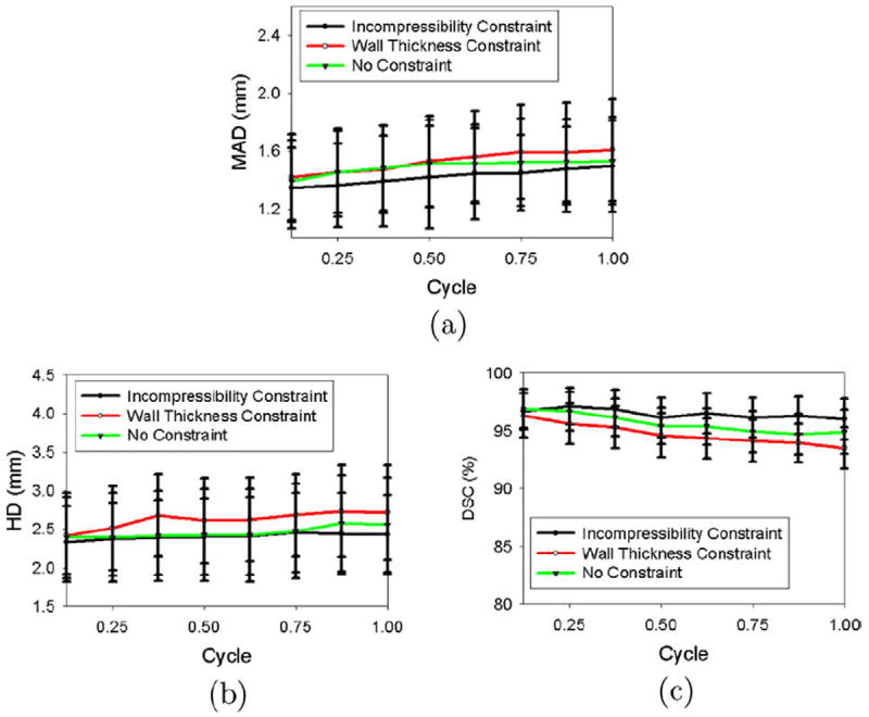
Segmentation errors of the endocardial (ENDO) contours for real images as functions of time over the cardiac cycle. (a) Mean absolute distance (MAD), (b) Hausdorff distance (HD), (c) Dice Similarity Coefficient (DSC).

Fig. 16.

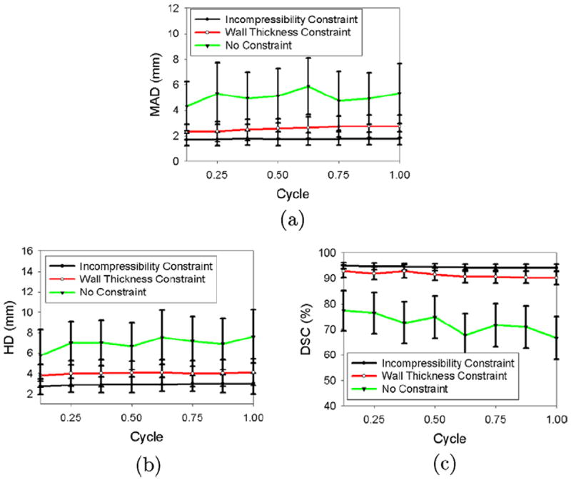
Segmentation errors of the epicardial (EPI) contours for real images as functions of time over the cardiac cycle. (a) Mean absolute distance (MAD), (b) Hausdorff distance (HD), (c) Dice Similarity Coefficient (DSC).

To further investigate the local segmentation errors, we used the 17-segment model, as described in Section 7.1, to compute the regional mean absolute distance (MAD)s on different sectors of the endocardial (ENDO) and epicardial (EPI) surfaces, as shown in Tables 4 and 5, respectively. We observed that the incompressibility constraint did not significantly improve the segmentation results for the endocardial (ENDO) surface. Also, we noticed that the mid-cavity mean absolute distance (MAD) was 1.36 mm, while the mean absolute distance (MAD)s for the basal and apical slices were 1.48 mm and 1.54 mm, respectively. This implies that the mid-cavity slices were relatively easier to segment than the basal and apical slices. This is probably due to the relatively higher intensity contrast in the mid-cavity slices compared to that in the basal and apical slices.

Table 4.

Comparison of regional endocardial (ENDO) mean absolute distance (MAD)s on real data (in mm).

		No constraint	Wall thickness constraint	IncompressibiLity constraint
BA	A	1.48 ± 0.28	1.46 ± 0.31	1.41 ± 0.28
	AL	1.52 ± 0.29	1.51 ± 0.29	1.43 ± 0.29
	IL	1.50 ± 0.33	1.49 ± 0.27	1.46 ± 0.31
	I	1.53 ± 0.31	1.51 ± 0.29	1.44 ± 0.31
	IS	1.47 ± 0.29	1.49 ± 0.30	1.40 ± 0.28
	AS	1.38 ± 0.26	1.47 ± 0.27	1.39 ± 0.28
MC	A	1.34 ± 0.20	1.51 ± 0.29	1.31 ± 0.21
	AL	1.45 ± 0.25	1.62 ± 0.31	1.45 ± 0.25
	IL	1.41 ± 0.28	1.57 ± 0.26	1.34 ± 0.24
	I	1.52 ± 0.30	1.64 ± 0.31	1.45 ± 0.29
	IS	1.41 ± 0.30	1.52 ± 0.27	1.35 ± 0.30
	AS	1.41 ± 0.29	1.51 ± 0.25	1.31 ± 0.26
AP	A	1.65 ± 0.35	1.61 ± 0.34	1.58 ± 0.34
	L	1.64 ± 0.31	1.58 ± 0.34	1.50 ± 0.32
	I	1.62 ± 0.27	1.56 ± 0.28	1.52 ± 0.31
	S	1.59 ± 0.33	1.58 ± 0.31	1.57 ± 0.31

BA: basal, MC: mid-cavity, AP: apical, A: anterior, AL: anterolateral, IL: inferolateral, I: inferior, IS: inferoseptal, AS: anteroseptal, L: lateral, S: septal.

Table 5.

Comparison of regional epicardial (EPI) mean absolute distance (MAD)s on real data (in mm).

		No constraint	Wall thickness constraint	Inconipressibility constraint
BA	A	6.13 ± 2.22	2.07 ± 0.58	1.79 ± 0.55
	AL	6.01 ± 2.01	2.11 ± 0.60	1.81 ± 0.69
	IL	5.91 ± 2.32	2.22 ± 0.67	1.80 ± 0.57
	I	5.61 ± 2.31	2.08 ± 0.84	1.78 ± 0.55
	IS	3.13 ± 1.25	2.04 ± 0.64	1.62 ± 0.43
	AS	3.75 ± 1.07	2.10 ± 0.67	1.61 ± 0.41
MC	A	5.32 ± 2.15	2.79 ± 1.05	1.78 ± 0.50
	AL	5.12 ± 2.42	3.37 ± 1.12	1.81 ± 0.53
	IL	5.01 ± 2.15	2.56 ± 0.97	1.75 ± 0.45
	I	4.99 ± 1.12	3.23 ± 0.98	1.78 ± 0.49
	IS	3.01 ± 0.99	2.61 ± 0.88	1.54 ± 0.41
	AS	3.12 ± 1.01	2.57 ± 0.64	1.55 ± 0.43
AP	A	6.12 ± 1.52	2.99 ± 1.32	1.85 ± 0.52
	L	6.11 ± 1.64	2.92 ± 1.12	1.89 ± 0.61
	I	6.18 ± 1.54	2.89 ± 1.24	1.81 ± 0.51
	S	6.22 ± 1.54	2.71 ± 1.28	1.80 ± 0.50
APX	APX	6.27 ± 1.55	2.92 ± 1.31	1.90 ± 0.54

BA: basal, MC: mid-cavity, AP: apical, APX: apex, A: anterior, AL: anterolateral, IL: inferolateral, I: inferior, IS: inferoseptal, AS: anteroseptal, L: lateral, S: septal.

Table 5 presents regional mean absolute distance (MAD)s for the epicardial (EPI) surfaces. When no constraint was applied, the regional mean absolute distance (MAD)s for the anterior, lateral, and inferior sectors were much larger than the regional mean absolute distance (MAD)s for the septal sector. It is so because the myocardium and its neighborhood tissues (such as liver) have similar intensities, making the free wall portion of the epicardial (EPI) contour ambiguous. The regional mean absolute distance (MAD)s at the inferolateral and anteroseptal sectors were relatively smaller due to the higher contrast between the left ventricular (LV) myocardium and the right ventricular (RV) blood pool. However, the epicardial (EPI) contour at the inferoseptal and anteroseptal sectors might leak due to the presence of the left ventricular (LV)/right ventricular (RV) junctures. This explains why the mean absolute distance (MAD)s of the epicardial (EPI) contour at the inferoseptal and anteroseptal sectors were still larger than the mean absolute distance (MAD)s of the corresponding endocardial (ENDO) contour.

When the wall thickness constraint was applied, the regional mean absolute distance (MAD)s for the anterior, anterolateral, inferolateral, and inferior sectors decreased by 1.65–4.06 mm, while the regional mean absolute distance (MAD)s for the inferoseptal and anteroseptal sectors decreased by 0.4–1.76 mm. However, the regional mean absolute distance (MAD)s for the mid-ventricular anterolateral and inferior sectors were still larger than those for other sectors (mean absolute distance (MAD) = 3.37 for the mid-ventricular anterolateral sector and 3.23 mm for the mid-ventricular inferior sector). This was due to the presence of the papillary muscles, which created the inhomogeneities in the wall thickness in these sectors. When the incompressibility constraint was applied, the mean absolute distance (MAD) decreased by 1.56 mm for the mid-ventricular anterolateral sector and by 1.45 mm for the mid-ventricular inferior sector.

As explained in Section 6.1, the real data included both normal and post-infarcted sequences. As shown in Tables 6 and 7, the wall thickness constraint produced endocardial (ENDO) contour results with similar accuracy for both the normal and the post-infarcted data, although the results from the normal data were slightly better. In contrast, for epicardial (EPI) contours, the mean absolute distance (MAD) and Hausdorff distance (HD) from post-infarcted data (mean absolute distance (MAD) = 2.86 mm and Hausdorff distance (HD) = 4.63 mm) were larger than those from the normal data (mean absolute distance (MAD) = 2.25 mm and Hausdorff distance (HD) = 3.41 mm), as shown in Tables 8 and 9. This is because the infarcted myocardial wall is usually thinner than the normal myocardial wall. When the incompressibility constraint was applied, however, the mean absolute distance (MAD), Hausdorff distance (HD), and Dice Similarity Coefficient (DSC) from the normal data (mean absolute distance (MAD) = 1.77 mm, Hausdorff distance (HD) = 2.97 mm, and Dice Similarity Coefficient (DSC) = 93.78%) were close to those from the post-infarcted data (mean absolute distance (MAD) = 1.71 mm, Hausdorff distance (HD) = 2.85 mm, and Dice Similarity Coefficient (DSC) = 94.02%). This implies that the deformable model with the incompressibility constraint can segment both normal and infarcted hearts with a similar accuracy, because it imposes a constraint on the myocardial volume (MV) while still allowing variations in the wall thickness.

Table 6.

Comparison of endocardial (ENDO) segmentation results on normal and post-infarcted hearts with incompressibility constraint.

	Normal	Post-infarcted
MAD (mm)	1.40 ± 0.28	1.45 ± 0.31
HD (mm)	2.52 ± 0.49	2.35 ± 0.47
DSC (%)	96.56 ± 1.60	95.98 ± 1.65

Table 7.

Comparison of endocardial (ENDO) segmentation results on normal and post-infarcted hearts with wall thickness constraint.

	Normal	Post-infarcted
MAD (mm)	1.49 ± 0.24	1.59 ± 0.32
HD (mm)	2.51 ± 0.52	2.73 ± 0.61
DSC (%)	95.29 ± 1.79	93.69 ± 2.00

Table 8.

Comparison of epicardial (EPI) segmentation results on normal and post-infarcted hearts with incompressibility constraint.

	Normal	Post-infarcted
MAD (mm)	1.77 ± 0.52	1.71 ± 0.40
HD (mm)	2.97 ± 0.78	2.85 ± 0.82
DSC (%)	93.78 ± 1.26	94.02 ± 1.37

Table 9.

Comparison of epicardial (EPI) segmentation results on normal and post-infarcted hearts with wall thickness constraint.

	Normal	Post-infarcted
MAD (mm)	2.25 ± 0.69	2.86 ± 0.79
HD (mm)	3.41 ± 0.92	4.63 ± 1.22
DSC (%)	92.41 ± 2.31	90.17 ± 2.62

In addition, we performed Bland–Altman analysis (Bland and Altman, 1986) to assess the agreement of myocardial volume (MV) measurements from manual segmentation and automatic segmentation. As shown in Fig. 17, the Bland–Altman plot revealed a large bias (bias = 18%) and 95% confidence interval²(95% confidence interval = [−10.4%,46.5%]) when no constraint was applied. The bias decreased (bias = 7.7%, −7.1%, and −5.8% for three observers) when the wall thickness constraint was applied. The bias further decreased (bias = 1.1%, 0.5%, and −0.8% for three observers) when the incompressibility constraint was applied. The 95% confidence interval with the incompressibility constraint (95% confidence interval = [−5.3%,7.6%], [−7.8%,8.9%], and [−8.2%,6.7%] for three observers, respectively) were also smaller compared to those obtained using the wall thickness constraint (95% confidence interval = [−21.7%,6.2%], [−22.3%,8.1%], and [−20.6%,8.9%] for three observers, respectively). This implies that the myocardial volume (MV)s obtained using the wall thickness constraint varied during a cardiac cycle, while the myocardial volume (MV)s obtained using the incompressibility constraint were nearly constant during the cycle.

Fig. 17.

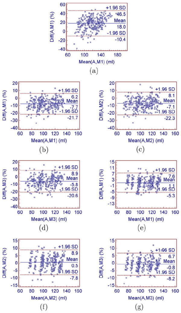
Bland–Altman analysis showing the agreement between the myocardial volume (MV) measurements from manual segmentation and automatic segmentation. (a) without the incompressibility constraint: automatic–manual 1, (b) with the wall thickness constraint: automatic–manual 1, (c) with the wall thickness constraint: automatic–manual 2, (d) with the wall thickness constraint: automatic–manual 3, (e) with the incompressibility constraint: automatic–manual 1, (f) with the incompressibility constraint: automatic–manual 2, (g) with the incompressibility constraint: automatic–manual 3.

8. Discussion

8.1. Sensitivity analysis

8.1.1. thin-plate spline (TPS) Control Points

To investigate the effects of the number of thin-plate spline (TPS) control points on the segmentation results, we randomly selected two real cardiac sequences, one from the normal data and the other from the post-infarcted data. Fig. 18 compares the segmentation performance with difference number of control points. The segmentation accuracy increased with number of control points, because more control points could better capture local shape features. The downside of using more control points, however, is that it makes the algorithm more expensive. Fig. 18a and c show that the mean absolute distance (MAD) curve for the endocardial (ENDO) surface became nearly flat when over 100 control points were used for the first sequence or when over 75 control points were used for the second sequence. The Hausdorff distance (HD) curve for the endocardial (ENDO) surface became nearly flat when over 125 control points were used for the first sequence or when over 100 control points were used for the second sequence. This implies that Hausdorff distance (HD) is more sensitive to control points as it reflects the local segmentation accuracy. Fig. 18b and d show that the mean absolute distance (MAD) curve for the epicardial (EPI) surface became nearly flat when over 100 control points were used for the first sequence or when over 75 control points were used for the second sequence. The Hausdorff distance (HD) curve for the epicardial (EPI) surface became nearly flat when over 100 control points were used for the first sequence or when over 100 control points were used for the second sequence. This implies that the epicardial (EPI) surface is less sensitive to the number of control points because it is less curved than the endocardial (ENDO) surface. As a tradeoff between speed and accuracy, we placed around 150 control points on the endocardial (ENDO) surface and 135 control points on the epicardial (EPI) surface.

Fig. 18.

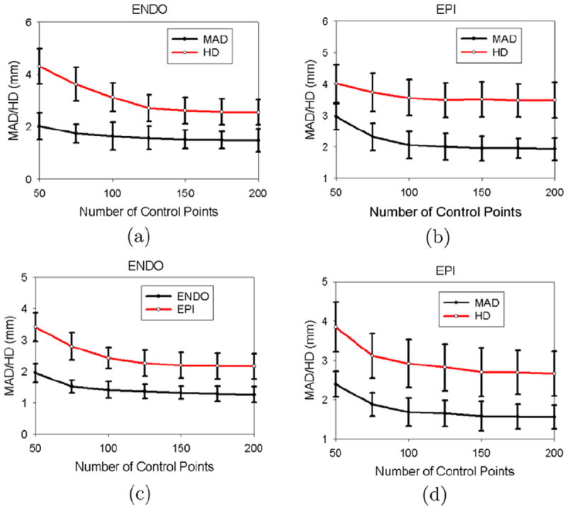
Sensitivity to the number of thin-plate spline (TPS) control points. (a,b) First sequence, (c,d) second sequence. (a,c) Fixed 135 control points on the epicardial (EPI) surface. (b,d) Fixed 150 control points on the endocardial (ENDO) surface.

8.1.2. The thin-plate spline (TPS) regularization parameter

As mentioned in Section 5.2, we used a regularization parameter λ to control the stiffness of thin-plate spline (TPS) warping. In practice, we used a stiff-to-flexible strategy, in which λ starts with an initial value λ^initial and then gradually decreases by a scaling factor γ until convergence. To investigate the effects of the initial value λ^initial and the scaling factor γ on the segmentation results, we randomly selected two real sequences, one from the normal data and the other from the post-infarcted data, and compared the segmentation accuracies with different λ^initial’s and γ’s. Fig. 19a and b show that the mean absolute distance (MAD) increased significantly when λ^initial < 1.5 for the first sequence or λ^initial < 3 for the second sequence. This is because a small λ produces too flexible a transform which is sensitive to image noise. Fig. 19c and d show that the mean absolute distance (MAD) increases when γ = 1 (i.e. constant λ). This is because the transform with a constant large λ produces a nearly pure affine transform which fails to capture local shape features. In addition, the mean absolute distance (MAD) increased significantly for the endocardial (ENDO) contour when γ > 2.5 for the first sequence or γ > 2 for the second sequence. For the epicardial (EPI) contour, the mean absolute distance (MAD) increased when γ > 2 for the first sequence or γ > 1.5 for the second sequence. This implies that the epicardial (EPI) contour needs a larger λ because the epicardial (EPI) contour is less curved than the endocardial (ENDO) contour. In practice, we set λ^initial = 3 and γ = 2 for the endocardial (ENDO) contour, and γ = 1.2 for the epicardial (EPI) contour.

Fig. 19.

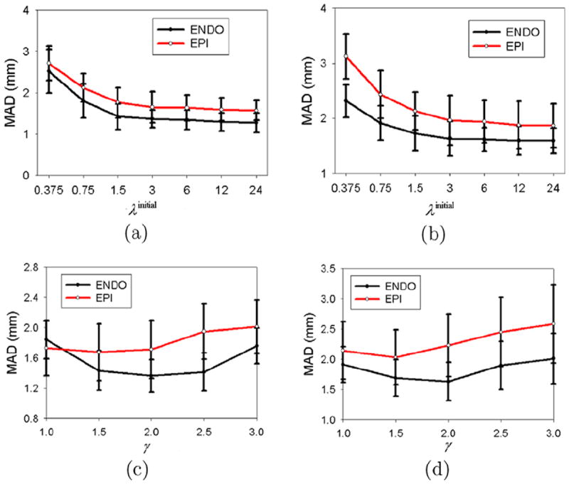
Sensitivity to the thin-plate spline (TPS) regularization parameter. (a) First sequence with γ = 2 for the endocardial (ENDO) contour and γ = 1.2 for the epicardial (EPI) contour, (b) Second sequence with γ = 2 for the endocardial (ENDO) contour and γ = 1.2 for the epicardial (EPI) contour, (c) First sequence with λ^initial = 3, (d) Second sequence with λ^initial = 3.

8.2. Clinical data

In this work, we validated our approach on canine real-time 3-D (RT3D) echocardiographic images. While the experimental results show that our model outperformed the deformable models with no constraint and with the wall thickness constraint, possible challenges might exist on how to analyze “low-quality” clinical data with low contrast and ambiguous myocardial boundaries.

These challenges are threefold. First, it becomes harder for observers to manually outline the endocardial (ENDO) and epicardial (EPI) contours of the first frame, from which our algorithm starts. One potential solution is to build a statistical model for the first frame (i.e. the end-diastole (ED) frame) from high quality magnetic resonance (MR) images. We can first rigidly transform (which is more robust) the model to fit the ultrasound image, and then automatically/manually adjust the weights associated with different modes of shape variations (which are obtained from the shape model) to match (partial) local features.

Second, the performance of the automatic algorithm might degrade with image quality. For example, local shape features (e.g. papillary muscles) might be compromised by poor image quality, leading to an over-smoothed segmentation of the endocardial (ENDO) boundaries. As well, the endocardial (ENDO) and epicardial (EPI) boundaries might be partially missing, due to signal dropout caused by the orientation dependence of image acquisition (Qian et al., 2006). Several potential solutions to this problem exist. The first solution is to increase the regularization parameter λ to make the thin-plate spline (TPS) warping more rigid and robust to noise. However, with a large λ, the segmented contours might fail to capture local shape features. The second solution is to add a shape prior to the segmentation process (Paragios, 2003). The third solution is to introduce a dropout prior that would bridge and detect signal dropout (Qian et al., 2006). Qian et al. have successfully applied a dropout prior to segment two-dimensional (2-D) echocardiographic images with signal dropout (Qian et al., 2006). Further extension to three-dimensional (3-D) images is still underway. We expect that the combination of the incompressibility constraint with a dropout prior will further improve the robustness of our algorithm.

Third, validation of “low-quality” data might be challenging. In this paper, we validated our approach against the manual segmentation from three observers. While this is sufficient for our data sets, it might not be adequate for low-quality images, from which manual segmentation is difficult. Further research on validation on low-quality data sets is a direction of future work.

8.3. Field of view

The proposed method assumes that the entire myocardium is captured in the field of view (FOV) for the entire cycle. However, it is possible that part of the epicardial (EPI) boundary will fall out of the field of view (FOV) in some phases of the cycle. Two potential solutions can be proposed to overcome this difficulty. First, the Philips IE33 system provides a “Live three-dimensional (3-D)” model, which offers real-time three-dimensional (3-D) rendering of a full volumetric view of the heart. This allows the operator to see, slice-by-slice, whether the entire epicardial (EPI) boundary falls into the field of view (FOV), prior image acquisition. If part of the boundary falls out of the field of view (FOV), one can adjust the position/angle of the probe to obtain the optimal acoustic window that captures the entire myocardium. Second, we can acquire volumetric images from different angles and fuse them to extend the field of view (FOV) (Rajpoot et al., 2009). We can then apply our algorithm to segment the fused volumetric data.

9. Conclusion

In this paper, we have presented a coupled deformable model for segmentation of the full myocardial volume from real-time 3-D (RT3D) echocardiographic images. The main contribution is the use of an incompressibility constraint for epicardial (EPI) border detection, which is more challenging than endocardial (ENDO) segmentation.

The incorporation of this incompressibility property into the segmentation process was formulated in a maximum a posteriori (MAP) framework, which consisted of a data adherence term and an incompressibility constraint. When defining the data adherence term, we took advantage of ultrasound physics and modeled the speckle statistics using the Nakagami distribution. In the incompressibility constraint term, we modeled the myocardial volume (MV) with a Gaussian distribution by noticing that the myocardial volume (MV) varies less than 5% during a cardiac cycle.

To validate this algorithm, we employed three independent observers and qualitatively and quantitatively compared the results from automatic segmentation with those from manual segmentation. While the endocardial (ENDO) contours could be detected with sufficient accuracy, even without the incompressibility constraint, the epicardial (EPI) contour leaked into the background. When the incompressibility constraint was applied, however, the automatic segmentation produced results with comparable accuracy to a manual segmentation. To further explore the distribution of local segmentation errors, we computed the regional mean absolute distance (MAD)s from each sector of the myocardium defined by a 17-segment model.

In addition, we compared the segmentation results obtained with a wall thickness constraint and an incompressibility constraint. The segmentation results obtained with the wall thickness constraint were more accurate than those obtained with no constraint, because the epicardial (EPI) boundary did not leak into the background. Nevertheless, the epicardial (EPI) contours using a wall thickness constraint were less accurate in the regions with inhomogeneous wall thickness. When the incompressibility constraint was applied, however, the epicardial (EPI) contours were correctly segmented in the regions with inhomogeneous wall thickness.

Future work includes the integration of segmentation and motion analysis into a unified system. While segmentation results can help to determine the deformation of the endocardial (ENDO) and epicardial (EPI) surfaces, the deformation of the endocardial (ENDO) and epicardial (EPI) surfaces can in turn be used for segmentation.

Appendix A. Pearson chi-squared goodness-of-fit test

Pearson chi-squared goodness-of-fit test is a commonly used statistical procedure that assesses whether an observed frequency distribution comes from a particular theoretical distribution.

Suppose we are given n independent observations x₁,x₂,…,x_n to form a histogram of M bins, and we want to test whether these n observations follow a theoretical distribution p(x∣θ), where θ is the vector of distribution’s parameters. Let m_i be the number of observed points falling into bin i. Then

$$p_i={\mathit{\int }}_{{\mathrm{bin}}_i}p(x\mid \theta )\mathit{dx}$$

is the probability of x falling into bin i. The statistics:

$${\chi }_s^2=\sum _{i=1}^M\frac{{(m_i-n{p}_i)}^2}{n{p}_i}$$

is therefore a measure of deviation of samples from expectations. Pearson proved that the limiting distribution ${\chi }_s^2$ has a chi-squared distribution with a degree of freedom of M-L-1, where L is the number of parameters estimated. Hence, the corresponding significance values of each fitting can be identified by finding the tail of χ²(M-L-1), i.e.

$$p={\mathit{\int }}_{{\chi }_s^2}^{+\infty }{\chi }^2(M-L-1)\mathit{dx}$$

Appendix B. Thin-plate spline warping

The thin-plate spline (TPS) warping is a composition of an affine transform and a non-rigid warping. Consider K control points $\Theta ={\{P_i\}}_{i=1}^k$ located on the surface of the source shape, the thinplate spline (TPS) warping is defined as

$${\mathbf{x}}^{\prime }=[ATW]\left[\begin{array}{c}\mathbf{x}\\ 1\\ U(\Vert \mathbf{x}-\Theta \Vert )\\ \end{array}\right]$$ (B.1)

where A ∈ ℝ^3×3 and T ∈ ℝ^3×1 represent the affine part of the thinplate spline (TPS) warping, and W ∈ ℝ^3×k is the weight matrix of non-rigid warping. U(r) = −|r| is the radial basis of the three-dimensional (3-D) spline.

Constraints on the square integrability of the second derivatives of the spline-based interpolation functions give the following additional relationship

$$W[\Theta \mathbf{1}]=\mathit{WQ}=\mathbf{0}$$ (B.2)

where 1 ∈ ℝ^K×1 and 0 ∈ ℝ^3×4. Combining Eqs. B.1 and B.2, one could write

$$[\Theta 0]=[ATW]\left[\begin{array}{cc}{Q}^T& 0\\ Z& Q\end{array}\right]$$

where Z_ij = U(∥P_i − P_j∥) and 0 is a zero matrix∈ ℝ^4×4. The warping model in Eq. (B.1) can therefore be parameterized only in terms of Θ, via a linear mapping

$$\begin{array}{l}{\mathbf{x}}^{\prime }=L(\mathbf{x};\Theta )=[\Theta 0]{\left[\begin{array}{cc}{Q}^T& 0\\ Z& Q\end{array}\right]}^{-1}\\ \left[\begin{array}{c}\mathbf{x}\\ \mathbf{1}\\ U(\Vert \mathbf{x}-\Theta \Vert )\end{array}\right]\end{array}$$

The linear relation makes efficient the computation of Jacobian of the warp $\frac{\partial L(\mathbf{x};\Theta )}{\partial \Theta }$. To regularize the thin-plate spline (TPS) warping, we use a stiff-to-flexible approach, as suggested in (Lim and Yang, 2005), consisting of replacing the matrix Z with Z + λI, where I is the identity matrix. We start with some large λ to force the warp to be rigid, and then repeat with smaller λ’s to capture local non-rigid deformations until we have a good estimate.

Appendix C. Derivation of Eqs. (8) and (9)

Let H(·) denote the Heaviside function, and δ(·) denote the Dirac function (Chan and Vese, 2001), i.e.

$$\begin{array}{l}H(\varphi )=\{\begin{array}{cc}1& \mathrm{if}\varphi \ge 0\\ 0& \mathrm{if}\varphi <0\end{array}\\ \delta (\varphi )=\frac{\mathit{dH}}{\mathit{d\varphi }}(\varphi )\end{array}$$

First, we use the Heaviside function to rewrite the integral inside the blood pool (i.e. Ω₁) as an integral over the entire image domain (i.e. $\Omega ={\cup }_{l=1}^3{\Omega }_l$)

$${\mathit{\int }}_{{\Omega }_1}\log P_1(I)d\mathbf{x}={\mathit{\int }}_{\Omega }\log P_1(I)(1-H({\varphi }_{\mathrm{in}}))d\mathbf{x}$$ (C.1)

Similarly, we have

$${\mathit{\int }}_{{\Omega }_2}\log P_2(I)d\mathbf{x}={\mathit{\int }}_{\Omega }\log P_2(I)(H({\varphi }_{\mathrm{in}})-H({\varphi }_{\mathrm{out}}))d\mathbf{x}$$ (C.2)

$${\mathit{\int }}_{{\Omega }_3}\log P_3(I)d\mathbf{x}={\mathit{\int }}_{\Omega }\log P_3(I)H({\varphi }_{\mathrm{out}})d\mathbf{x}$$ (C.3)

For simple notation, we denote $E_1=\log P(I\mid {\varphi }_{\mathrm{in}},{\varphi }_{\mathrm{out}})={\sum }_{l=1}^3{\mathit{\int }}_{{\Omega }_l}\log P_l(I)d\mathbf{x}$. By plugging ${\varphi }_{\mathrm{in}}(\mathbf{x})={\varphi }_{\mathrm{in}}^0(L(\mathbf{x};{\Theta }_{\mathrm{in}}))$ into Eqs. (C.1) and (C.2), and taking the gradient of E₁ with respect to Θ_in using the chain rule, we have

$$\frac{\partial E_1}{\partial {\Theta }_{\mathrm{in}}}=-{\mathit{\int }}_{\Omega }\left\{\log \frac{P_1}{P_2}·\nabla {\varphi }_{\mathrm{in}}({\mathbf{x}}^{\prime })·\frac{\partial L}{\partial {\Theta }_{\mathrm{in}}}(\mathbf{x};{\Theta }_{\mathrm{in}})\right\}\delta ({\varphi }_{\mathrm{in}}^0(L(\mathbf{x};{\Theta }_{\mathrm{in}})))d\mathbf{x}$$ (C.4)

Since the Dirac function δ(·) prunes out everything in the image domain Ω, except on the zero level set boundary, i.e. $\{\mathbf{x}\mid {\varphi }_{\mathrm{in}}(\mathbf{x})={\varphi }_{\mathrm{in}}^0(L(\mathbf{x};{\Theta }_{\mathrm{in}}))=0\}$, we can reduce the volume integral in Eq. (C.4) to a surface integral as follows:

$$\frac{\partial E_1}{\partial {\Theta }_{\mathrm{in}}}=-{\mathit{\int }}_{\partial C_{12}}\left\{\log \frac{P_1}{P_2}·\nabla {\varphi }_{\mathrm{in}}({\mathbf{x}}^{\prime })·\frac{\partial L}{\partial {\Theta }_{\mathrm{in}}}(\mathbf{x};{\Theta }_{\mathrm{in}})\right\}d\mathbf{x}$$ (C.5)

where δC₁₂ is the interface between Ω₁ and Ω₂, i.e. the endocardial (ENDO) surface.

Similarly, we have

$$\frac{\partial E_1}{\partial {\Theta }_{\mathrm{out}}}=-{\mathit{\int }}_{\partial C_{23}}\left\{\log \frac{P_2}{P_3}·\nabla {\varphi }_{\mathrm{out}}(\mathbf{x}\prime )·\frac{\partial L}{\partial {\Theta }_{\mathrm{out}}}(\mathbf{x};{\Theta }_{\mathrm{out}})\right\}d\mathbf{x}$$ (C.6)

where ∂C₂₃ is the interface between Ω₂ and Ω₃, i.e. the epicardial (EPI) surface.

Second, we denote $E_2=\log P({\varphi }_{\mathrm{in}},{\varphi }_{\mathrm{out}})=-\frac{{\left({\mathit{\int }}_{{\Omega }_2}d\mathbf{x}-V_0\right)}^2}{2{\sigma }_0^2}+C$ (where C is a constant). By using the Heaviside function, we can rewrite it as

$$E_2=-\frac{{\{{\mathit{\int }}_{\Omega }(H({\varphi }_{\mathrm{in}})-H({\varphi }_{\mathrm{out}}))d\mathbf{x}-V_0\}}^2}{2{\sigma }_0^2}+C$$

Similarly to E₁, we take derivative of E₂ with respect to Θ_in and Θ_out, and arrive at

$$\frac{\partial E_2}{\partial {\Theta }_{\mathrm{in}}}=-\frac{V-V_0}{{\sigma }_0^2}{\mathit{\int }}_{\partial C_{12}}\nabla {\varphi }_{\mathrm{in}}({\mathbf{x}}^{\prime })\frac{\partial L}{\partial {\Theta }_{\mathrm{in}}}(\mathbf{x};{\Theta }_{\mathrm{in}})d\mathbf{x}$$ (C.7)

$$\frac{\partial E_2}{\partial {\Theta }_{\mathrm{out}}}=\frac{V-V_0}{{\sigma }_0^2}{\mathit{\int }}_{\partial C_{23}}\nabla {\varphi }_{\mathrm{out}}({\mathbf{x}}^{\prime })\frac{\partial L}{\partial {\Theta }_{\mathrm{out}}}(\mathbf{x};{\Theta }_{\mathrm{out}})d\mathbf{x}$$ (C.8)

Third, we combine Eqs. (C.5)-(C.7), (and) (C.8), and use gradient descent method, leading to the following evolution equations

$$\frac{\partial {\Theta }_{\mathrm{in}}}{\partial \tau }={\mathit{\int }}_{\partial C_{12}}\left(\log \frac{P_1}{P_2}+\frac{V-V_0}{{\sigma }_0^2}\right)\nabla {\varphi }_{\mathrm{in}}({\mathbf{x}}^{\prime })\frac{\partial L}{\partial {\Theta }_{\mathrm{in}}}(\mathbf{x};{\Theta }_{\mathrm{in}})d\mathbf{x}$$

$$\frac{\partial {\Theta }_{\mathrm{out}}}{\partial \tau }={\mathit{\int }}_{\partial C_{23}}\left(\log \frac{P_2}{P_3}-\frac{V-V_0}{{\sigma }_0^2}\right)\nabla {\varphi }_{\mathrm{out}}({\mathbf{x}}^{\prime })\frac{\partial L}{\partial {\Theta }_{\mathrm{out}}}(\mathbf{x};{\Theta }_{\mathrm{out}})d\mathbf{x}$$

where τ is the time step.

Appendix D. Parameter estimation for the mixture model

Suppose that data x₁,…, x_N comes from the mixture model

$$P(x;\Phi )=\sum _{k=1}^M{\alpha }_k{P}_k(x;{\mu }_k,{\omega }_k)$$ (D.1)

where M is the number of components, α_k is the mixture proportion of component k, P_k(x; μ_k, ω_k) is the kth component Nakagami distribution parameterized by μ_k and ω_k. We want to use the Expectation–Maximization (EM) algorithm to estimate the parameter vector Φ = (α_k, μ_k,ω_k ∣k = 1,…,M) of the mixture model.

We augment the data x₁,…,x_N by an unobservable matrix z_ik,i = 1,…,N;k = 1,…,M. The values of z_ik are indicators, defined as

$$\begin{array}{l}\\ z_{\mathit{ik}}=\{\begin{array}{ll}1,& x_i\mathrm{comes\; from\; the\; distribution}{P}_k\\ 0,& \mathrm{else}\end{array}\end{array}$$ (D.2)

The unobservable matrix z_ik tells us where the ith observation x_i comes from. With the augmented data, the complete likelihood takes a quite simple form

$$\prod _{i=1}^N\prod _{k=1}^M{({\alpha }_k{P}_k(x_i;{\mu }_k,{\omega }_k))}^{z_{\mathit{ik}}}$$ (D.3)

The complete log-likelihood is

$$\log L_c(\Phi )=\sum _{i=1}^N\sum _{k=1}^M{z}_{\mathit{ik}}(\log {\alpha }_k+\log P_k(x_i;{\mu }_k,{\omega }_k))$$ (D.4)

The Expectation–Maximization (EM) algorithm is applied to this problem by treating z_ik as missing data. It proceeds iteratively in two steps, the expectation step (E-step) and the maximization step (M-step). The expectation step (E-step) requires the calculation of the current conditional expectation of logL_c(Φ) given x, using Φ⁽ⁿ⁾ for Φ, which can be written as

$$Q(\Phi \mid {\Phi }^{(n)})=E_{z\mid x,{\Phi }^{(n)}}(\log L_c(\Phi ))$$ (D.5)

As the complete log-likelihood, logL_c(Φ), is linear in the unobservable data z_ik, the expectation step (E-step) simply requires the calculation of the current conditional expectation of z_ik, given the observed data x.

$$E_{z\mid x,{\Phi }^{(n)}}(z_{\mathit{ik}})=P(z_{\mathit{ik}}=1\mid \mathbf{x},{\Phi }^{(n)})=z_{\mathit{ik}}^{(n)}$$ (D.6)

where $z_{\mathit{ik}}^{(n)}$ is the posterior probability of the ith observation coming from the kth mixture component in the iteration step n.

$$z_{\mathit{ik}}^{(n)}=\frac{{\alpha }_k^{(n)}P(x_i;{\mu }_k^{(n)},{\omega }_k^{(n)})}{\sum _{k=1}^M{\alpha }_k^{(n)}P(x_i;{\mu }_k^{(n)},{\omega }_k^{(n)})}$$ (D.7)

Thus, we have

$$Q(\Phi \mid {\Phi }^{(n)})=\sum _{i=1}^N\sum _{k=1}^M{z}_{\mathit{ik}}^{(n)}(\log {\alpha }_k+\log P_k(x_i;{\mu }_k,{\omega }_k))$$ (D.8)

The maximization step (M-step) requires the global minimization of Q(Φ∣Φ⁽ⁿ⁾) with respect to Φ to give an updated estimate Φ⁽ⁿ⁺¹⁾. If the z_ik is observable, the complete data maximum likelihood estimation of α_k would be simply given by

$${\widehat{\alpha }}_k=\frac{1}{N}\sum _{i=1}^N{z}_{\mathit{ik}}$$ (D.9)

By replacing each z_ik with $z_{\mathit{ik}}^{(n)}$, we have

$${\alpha }_k^{(n+1)}=\frac{1}{N}\sum _{i=1}^N{z}_{\mathit{ik}}^{(n)}$$ (D.10)

To find the optimal ω_k, we take the derivative of Q(Φ∣Φ⁽ⁿ⁾) with respect to ω_k

$$\frac{\partial Q}{\partial {\omega }_k}=\frac{1}{N}\sum _{i=1}^N{z}_{\mathit{ik}}^{(n)}\left(-\frac{{\mu }_k}{{\omega }_k}+\frac{{\mu }_k}{{\omega }_k^2}{x}_i^2\right)=0$$ (D.11)

The optimal ω_k at the (n + 1)th iteration is ${\omega }_k^{(n+1)}=\frac{{\sum }_{i=1}^N{z}_{\mathit{ik}}^{(n)}{x}_i^2}{{\sum }_{i=1}^N{z}_{\mathit{ik}}^{(n)}}$.

To find the optimal μ_k, we take the derivative of Q(Φ∣Φ⁽ⁿ⁾) with respect to μ_k

$$\frac{\partial Q}{\partial {\mu }_k}=\frac{1}{N}\sum _{i=1}^N{z}_{\mathit{ik}}^{(n)}\left(1+\log {\mu }_k-\frac{{\Gamma }^{\prime }({\mu }_k)}{\Gamma ({\mu }_k)}-\log {\omega }_k+2\log x_i-\frac{x_i^2}{{\omega }_k}\right)=0$$ (D.12)

By using the approximation log ${\mu }_k-\frac{{\Gamma }^{\prime }({\mu }_k)}{\Gamma ({\mu }_k)}\approx \frac{1}{{\mu }_k}\left(\frac{1}{2}+\frac{1}{12{\mu }_k+2}\right)$, we obtain the optimal μ_k at the (n + 1)th iteration as follows:

$${\mu }_k^{(n+1)}=\frac{3-s+\sqrt{{(s-3)}^2+24s}}{12s}$$ (D.13)

where $s=\frac{{\sum }_{i=1}^N{z}_{\mathit{ik}}^{(n)}\left(\log {\omega }_k^{(n+1)}-2\log x_i+x_i^2/{\omega }_k-1\right)}{{\sum }_{i=1}^N{z}_{\mathit{ik}}^{(n)}}$.

References

- Angelsen BA. A theoretical study of the scattering of ultrasound from blood. IEEE TBME. 1980;27(2):61–67. doi: 10.1109/TBME.1980.326708. [DOI] [PubMed] [Google Scholar]
- Binder T, Sussner M, Moertl D, Strohmer H, Baumgartner T, Maurer G, Porenta G. Artificial neural networks and spatial temporal contour linking for automated endocardial contour detection on echocardiograms: a novel approach to determine left ventricular contractile function. Ultrasound Med Biol. 1999;25(7):1069–1076. doi: 10.1016/s0301-5629(99)00059-9. [DOI] [PubMed] [Google Scholar]
- Bistoquet A, Oshinski J, Shrinjar O. Myocardial deformation recovery from cine mri using a nearly incompressibile biventricular model. Med Image Anal. 2008;12:69–85. doi: 10.1016/j.media.2007.10.009. [DOI] [PubMed] [Google Scholar]
- Bland JM, Altman DG. Statistical methods for assessing agreement between two methods of clinical measurement. Lancet. 1986;i:307–310. [PubMed] [Google Scholar]
- Bosch JG, Mitchell SC, Lelieveldt BP, Nijland F, Kamp O, Sonka M, Reiber JHC. Automatic segmentation of echocardiographic sequences by active appearance motion model. IEEE TMI. 2002;21(11):1374–1383. doi: 10.1109/TMI.2002.806427. [DOI] [PubMed] [Google Scholar]
- Boukerroui D, Baskurt A, Noble JA, Basset O. Segmentation of ultrasound images – multiresolution 2d and 3d algorithm based on global and local statistics. Pattern Recogn Lett. 2003;24:779–790. [Google Scholar]
- Bowman AW, Kovacs SJ. Assessment and consequences of the constantvolume attribute of the four-chamber heart. Am J Physiol Heart Circ Physiol. 2003;285:H2027–2033. doi: 10.1152/ajpheart.00249.2003. [DOI] [PubMed] [Google Scholar]
- Cerqueira MD, Weissman NJ, Dilsizian V, Jacobs AK, Kaul S, Laskey WK, Pennell DJ, Rumberger JA, Ryan T, Varani MS. Standardized myocardial segmentation and nomenclature for tomographic imaging of the heart: a statement for healthcare professionals from the cardiac imaging committee of the concil on clinical cardiology of the american heart association. Circulation. 2002;105:539–542. doi: 10.1161/hc0402.102975. [DOI] [PubMed] [Google Scholar]
- Chalana V, Linker DT, Haynor DR, Kim Y. A multiple active contour model for cardiac boundary detection on echocardiographic sequences. IEEE TMI. 1996;15(3):290–298. doi: 10.1109/42.500138. [DOI] [PubMed] [Google Scholar]
- Chan TF, Vese LA. Active contours without edges. IEEE IP. 2001;10(2):266–277. doi: 10.1109/83.902291. [DOI] [PubMed] [Google Scholar]
- Chen X, Xie H, Erkamp R, Kim K, Jia C, Rubin J, O’Donnell M. 3-d correlation-based speckle tracking. Ultrason Imag. 2005;27:21–36. doi: 10.1177/016173460502700102. [DOI] [PubMed] [Google Scholar]
- Coppini G, Poli R, Valli G. Recovery of the 3-d shape of the left ventricle from echocardiographic images. IEEE TMI. 1995;14(2):301–317. doi: 10.1109/42.387712. [DOI] [PubMed] [Google Scholar]
- Davignon F, Deprez J-F, Basset O. A parametric imaging approach for the segmentation of ultrasound data. Ultrasonics. 2005;43:789–801. doi: 10.1016/j.ultras.2005.06.001. [DOI] [PubMed] [Google Scholar]
- Dickinson R, Hill C. Measurement of soft tissue motion using correlation between a-scans. Ultrasound Med Biol. 1982;8(3):263–271. doi: 10.1016/0301-5629(82)90032-1. [DOI] [PubMed] [Google Scholar]
- Duan Q, Angelini ED, Herz SL, Ingrassia CM, Costa KD, Holmes JW, Homma S, Laine AF. Region-based endocardium tracking on real-time three-dimensional ultrasound. Ultrasound Med Biol. 2009;35(2):256–265. doi: 10.1016/j.ultrasmedbio.2008.08.012. [DOI] [PMC free article] [PubMed] [Google Scholar]
- Dutt V, Greenleaf JF. Ultrasound echo envelop analysis using a homodyned K distribution signal model. Ultrason Imag. 1994;16:265–287. doi: 10.1177/016173469401600404. [DOI] [PubMed] [Google Scholar]
- Glass L, Hunter P, McCulloch A. Theory of Heart: Biomechanics, Biophysics, and Nonlinear Dynamics of Cardiac Function. Springer-Verlag; 1990. [Google Scholar]
- Hamilton WF, Rompf JH. Movement of the base of the ventricle and the relative constancy of the cardiac volume. Am J Physiol. 1932;132:559–565. [Google Scholar]
- Hoffman EA, Ritman EL. Invariant total heart volume in the intact thorax. Am J Physiol Heart Circ Physiol. 1985;249:H883–H890. doi: 10.1152/ajpheart.1985.249.4.H883. [DOI] [PubMed] [Google Scholar]
- Hoffman EA, Ritman EL. Heart-lung interaction: effect of regional lung air content and total heart volume. Ann Biomed Eng. 1987;15:241–257. doi: 10.1007/BF02584282. [DOI] [PubMed] [Google Scholar]
- Jacob G, Noble A, Behrenbruch C, Kelion AD, Banning AP. A shape-spacebased approach to tracking myocardial borders and quantifying regional leftventricular function applied in echocardiography. IEEE TMI. 2002;21(3):226–238. doi: 10.1109/42.996341. [DOI] [PubMed] [Google Scholar]
- Jakeman E. K-distributed noise. J Opt A: Pure Appl Opt. 1999;1:784–789. [Google Scholar]
- Jensen J. Field: a program for simulating ultrasound systems. Med Biol Eng Comput. 1996;34(Suppl. 1, Part 1):351–353. [Google Scholar]
- Jensen J, Svendsen N. Calculation of pressure fields from arbitrary shaped, apodized, and excited ultrasound transducers. IEEE Trans Ultrason Ferroelec Freq Contr. 1992;39:262–267. doi: 10.1109/58.139123. [DOI] [PubMed] [Google Scholar]
- Ledesma-Carbayo MJ, Kybic J, Desco M, Santos A, Suhling M, Hunziker P, Unser M. Spatio-temporal nonrigid registration for ultrasound cardiac motion estimation. IEEE TMI. 2005;24(9):1113–1126. doi: 10.1109/TMI.2005.852050. [DOI] [PubMed] [Google Scholar]
- Lim J, Yang M-H. A direct method for modeling non-rigid motion with thin plate spline. CVPR05. 2005;1:1196–1202. [Google Scholar]
- Lin N, Yu W, Duncan JS. Combinative multi-scale level set framework for echocardiographic image segmentation. Med Image Anal. 2003;7:529–537. doi: 10.1016/s1361-8415(03)00035-5. [DOI] [PubMed] [Google Scholar]
- Lynch M, Ghita O, Whelan P. Left-ventricle myocardium segmentation using a coupled level-set with a priori knowledge. Comput Med Imag Graph. 2006;30(4):255–262. doi: 10.1016/j.compmedimag.2006.03.009. [DOI] [PubMed] [Google Scholar]
- Malassiotis S, Strintzis MG. Tracking the left ventricle in echocardiographic images by learning heart dynamics. IEEE TMI. 1999;18(3):282–290. doi: 10.1109/42.764905. [DOI] [PubMed] [Google Scholar]
- Mansi T, Peyrat J-M, Sermesant M, Delingette H, Blanc J, Boudjemline Y, Anyache N. Physically-constrained diffeomorphic demons for the estimation of 3d myocardium strain from cine-mri. FIMH. 2009:201–210. [Google Scholar]
- Mignotte M, Meunier J, Tardif J-C. Endocardial boundary estimation and tracking in echocardiographic images using deformable template and markov random field. Pattern Anal Appl. 2001;24(4):256–271. [Google Scholar]
- Mulet-Parada M, Noble JA. 2d+t acoustic boundary detection in echocardiography. Med Image Anal. 2000;4:21–30. doi: 10.1016/s1361-8415(00)00006-2. [DOI] [PubMed] [Google Scholar]
- Myronenko A, Song X, Sahn DJ. Lv motion tracking from 3d echocardiography using textural and structural information. MICCAI. 2007:428–435. doi: 10.1007/978-3-540-75759-7_52. [DOI] [PubMed] [Google Scholar]
- Noble JA, Boukerroui D. Ultrasound image segmentation: a survey. IEEE TMI. 2006;25(8):987–1010. doi: 10.1109/tmi.2006.877092. [DOI] [PubMed] [Google Scholar]
- O’Donnell T, Funka-Lea G. 3-D cardiac volume analysis using magnetic resonance imaging. Proceedings of the Fourth IEEE Workshop on Applications of Computer Vision (WACV); 1998. pp. 240–241. [Google Scholar]
- Orderud F, Hansgard J, Rabben SI. Real-time tracking of the left ventricle in 3d echocardiography using a state estimation approach. MICCAI. 2007:858–865. doi: 10.1007/978-3-540-75757-3_104. [DOI] [PubMed] [Google Scholar]
- Papademetris X, Jackowski M, Rajeevan N, Okuda H, Constable RT, Staib LH. Section of Bioimaging Sciences, Dept of Diagnostic Radiology, Yale School of Medicine; 2006. Bioimage suite: An integrated medical image analysis suite. < http://www.bioimagesuite.org>. [PMC free article] [PubMed] [Google Scholar]
- Paragios N. A level set approach for shape-driven segmentation and tracking of the left ventricle. IEEE TMI. 2003;22(6):773–776. doi: 10.1109/TMI.2003.814785. [DOI] [PubMed] [Google Scholar]
- Philips. Philips Medical Systems Corporate Website. 2005 < http://www.medical.philips.com/main/products/ultrasound/cardiology/>.
- Qian X, Tagare HD, Tao Z. Segmentation of rat cardiac ultrasound images with large dropout regions. MMBIA 2006 [Google Scholar]
- Rajpoot K, Noble JA, Grau V. Multiview rt3d echocardiographic image fusion. FIMH. 2009:134–143. [Google Scholar]
- Saddi KA, Chefd’hotel C, Cheriet F. Large deformation registration of contrast-enhanced images with volume-preserving constraint. SPIE. 2007;6512 [Google Scholar]
- Sarti A, Corsi C, Mazzini E, Lamberti C. Maximum likelihood segmentation of ultrasound images with rayleigh distribution. IEEE TUFFC. 2005;52(6):947–960. doi: 10.1109/tuffc.2005.1504017. [DOI] [PubMed] [Google Scholar]
- Setarehdan SK, Soraghan JJ. Automatic cardiac lv boundary detection and tracking using hybrid fuzzy temporal and fuzzy multiscale edge detection. IEEE Trans Biomed Eng. 1999;46(11):1364–1378. doi: 10.1109/10.797997. [DOI] [PubMed] [Google Scholar]
- Shankar PM. A general statistical model for ultrasonic backscattering from tissues. IEEE UFFC. 2000;47(3):727–736. doi: 10.1109/58.842062. [DOI] [PubMed] [Google Scholar]
- Shung KK, Thieme GA. Ultrasonic Scattering in Biological Tissues. CRC; 1992. [Google Scholar]
- Song M, Haralick RM, Sheehan FH, Johnson RK. Integrated surface model optimization for freehand three-dimensional echocardiography. IEEE TMI. 2002;21(9):1077–1090. doi: 10.1109/TMI.2002.804433. [DOI] [PubMed] [Google Scholar]
- Tao Z, Tagare H, Beaty JD. Evaluation of four probability distribution models for speckle in clinical cardiac ultrasound images. IEEE TMI. 2006;25(11):1483–1491. doi: 10.1109/TMI.2006.881376. [DOI] [PubMed] [Google Scholar]
- Taron M, Paragios N, Jolly M-P. From uncertainties to statistical model building and segmentation of the left ventricle. MMBIA07 2007 [Google Scholar]
- Wagner RF, Smith SW, Sandrik JM, Lopez H. Statistics of speckle in ultrasound b-scans. IEEE Trans Sonics Ultrason. 1983;30(3):156–163. [Google Scholar]
- Yan P, Sinusas A, Duncan J. Lv segmentation from 3d echocardiography using fuzzy features and a multilevel ffd model. ISBI. 2007:848–851. [Google Scholar]
- Yang L, Georgescu B, Zheng Y, Foran DJ, Comaniciu D. A fast and accurate tracking algorithm of left ventricles in 3d echocardiography. ISBI. 2008:221–224. doi: 10.1109/ISBI.2008.4540972. [DOI] [PMC free article] [PubMed] [Google Scholar]
- Zhu Y, Papademetris X, Duncan J, Sinusas A. Cardiac mr segmentation with incompressibility constraint. ISBI. 2007a:185–188. [Google Scholar]
- Zhu Y, Papademetris X, Sinusas A, Duncan J. Segmentation of myocardial volumes from real-time 3d echocardiography using an incompressibility constraint. MICCAI. 2007b:44–51. doi: 10.1007/978-3-540-75757-3_6. [DOI] [PubMed] [Google Scholar]