Feature-Based Morphometry: Discovering Group-related Anatomical Patterns

Abstract

This paper presents feature-based morphometry (FBM), a new, fully data-driven technique for discovering patterns of group-related anatomical structure in volumetric imagery. In contrast to most morphometry methods which assume one-to-one correspondence between subjects, FBM explicitly aims to identify distinctive anatomical patterns that may only be present in subsets of subjects, due to disease or anatomical variability. The image is modeled as a collage of generic, localized image features that need not be present in all subjects. Scale-space theory is applied to analyze image features at the characteristic scale of underlying anatomical structures, instead of at arbitrary scales such as global or voxel-level. A probabilistic model describes features in terms of their appearance, geometry, and relationship to subject groups, and is automatically learned from a set of subject images and group labels. Features resulting from learning correspond to group-related anatomical structures that can potentially be used as image biomarkers of disease or as a basis for computer-aided diagnosis. The relationship between features and groups is quantified by the likelihood of feature occurrence within a specific group vs. the rest of the population, and feature significance is quantified in terms of the false discovery rate. Experiments validate FBM clinically in the analysis of normal (NC) and Alzheimer's (AD) brain images using the freely available OASIS database. FBM automatically identifies known structural differences between NC and AD subjects in a fully data-driven fashion, and an equal error classification rate of 0.80 is achieved for subjects aged 60-80 years exhibiting mild AD (CDR=1).

1. Introduction

Morphometry aims to automatically identify anatomical differences between groups of subjects, e.g. diseased or healthy brains. The typical computational approach taken to morphometry is a two step process. Subject images are first geometrically aligned or registered within a common frame of reference or atlas, after which statistics are computed based on group labels and measurements of interest (Kendall, 1989; Bookstein, 1989). Morpho-metric approaches can be contrasted according to the measurements upon which statistics are computed. Voxel-based morphometry (VBM) involves analyzing intensities or tissue class labels (Ashburner and Friston, 2000; Toga et al., 2001). Deformation or tensor-based morphometry (TBM) analyzes the deformation fields which align subjects (Ashburner et al., 1998; Thompson et al., 2000; Chung et al., 2001; Studholme et al., 2006; Lao et al., 2004). Object-based morphometry analyzes the deformation of specific pre-segmented anatomical structures of interest, e.g. cortical sulci (Mangin et al., 2004) or subcortical structures (Pohl and Sabuncu, 2009).

A fundamental assumption underlying most morphometry techniques is that inter-subject registration is capable of achieving one-to-one correspondence between subjects, and that statistics can therefore be computed from measurements of the same anatomical tissues across subjects. Inter-subject registration remains a major challenge, however, due to the fact that no two subjects are identical; the same anatomical structure may vary significantly or exhibit distinct, multiple morphologies across a population, or may not be present or easily identifiable in all subjects, e.g. in the case of different cortical folding patterns, or in the case of pathology. Coarse linear registration can be used to normalize images with respect to global geometrical differences, e.g. rotation and magnification, however cannot achieve precise alignment of fine anatomical structures. Deformable registration has the potential to refine the alignment of fine anatomical structures, however it is difficult to guarantee that images are not being over-aligned. Registration algorithms can be compared in terms of their ability to achieve overlap of segmented anatomical structures known to exist in healthy subjects (Klein et al., 2009; Hellier et al., 2003). Overlap measures are only a surrogate for registration accuracy, however, as different geometrical priors (e.g. fluid (Bro-Nielsen and Gramkow, 1996), elastic (Bajcsy and Kovacic, 1989)) will generally result in different registration solutions, which may simultaneously minimize volumetric overlap while remaining anatomically implausible. Furthermore, it is difficult to gauge registration performance when correspondence is ambiguous or non-existent. Consequently, it may be unrealistic and potentially detrimental to assume one-to-one correspondence, as morphometric analysis may be confounding image measurements arising from different underlying anatomical tissues (Bookstein, 2001; Ashburner and Friston, 2001; Davatzikos, 2004).

Various approaches have been proposed to cope with the lack of one-toone correspondence when registering or modeling images of multiple subjects. Images can be automatically clustered or divided into distinct subsets based on image content (Blezek and Miller, 2006; Sabuncu et al., In Press), however the assumption of one-to-one correspondence is operative during clustering and within subsets. Image regions containing group-informative measurements can be identified in an automatic manner (Fan et al., 2007), however one-to-one correspondence is assumed at a local scale. Inter-subject or atlas-to-subject correspondence can be expressed in terms of valid correspondence plus a residual component (Baloch et al., 2007), where the residual represents unexplainable correspondence error. This technique cannot effectively represent the case where the same local anatomical region or structure bears multiple, distinct, modes of appearance, e.g. multiple folding patterns associated with the same gyrus in the cortex (Ono et al., 1990). The difficulty in achieving correspondence can be mitigated by considering pre-defined anatomical structures known to exist in most subjects (Mangin et al., 2004; Pohl and Sabuncu, 2009), however such structures may not be known a priori or may be unrelated to the particular group phenomena of interest. Individual subjects can be matched to multiple atlases (Klein and Hirsch, 2005), however it is unclear how this strategy can be adapted to identify group-related anatomical structure. Several authors propose relating subjects in terms of localized features, e.g. geometrical structures (Coulon et al., 2000; Thirion et al., 2007), moment descriptors (Sun et al., 2007, 2008) or features combining local geometry and appearance (Toews and Arbel, 2007; Toews et al., 2009). Local features provide a mechanism for avoiding one-to-one correspondence throughout the image, particularly in the highly variable cortex (Sun et al., 2007; Toews et al., 2009).

Feature-based morphometry (FBM) is proposed specifically to avoid the assumption of one-to-one inter-subject correspondence. FBM admits that correspondence may not exist between all subjects and/or throughout the image, and instead attempts to identify distinctive, localized patterns of anatomical structure for which correspondence between subsets of subjects is statistically probable. Such patterns are identified and represented as distinctive scale-invariant features (Lowe, 2004; Mikolajczyk and Schmid, 2004), i.e. generic image patterns that can be automatically extracted in the image by a front-end salient feature detector. A probabilistic model quantifies feature variability in terms of appearance, geometry, and occurrence statistics relative to subject groups. Model parameters are estimated using a fully automatic, data-driven learning algorithm to identify local patterns of anatomical structure and quantify their relationships to subject groups. The local feature thus replaces the global atlas as the basis for morphometric analysis. Scale-invariant features are widely used in the computer vision literature for image matching, and have been extended to matching 3D volumetric medical imagery (Cheung and Hamarneh, 2007; Allaire et al., 2008). FBM follows from a line of research in which generic object appearance is modeled in terms of a collection of independently occurring local features in photographic imagery (Fergus et al., 2006) and in 2D slices of the brain (Toews and Arbel, 2007). FBM builds on this research, by extending the modeling theory to address group analysis and to operate in 3D volumetric imagery. FBM is generally applicable to arbitrary 3D imagery and subject groups; here as an example application, we choose to validate FBM in the analysis Alzheimer's disease (AD), an important and heavily-studied neurological disease.

The remainder of this paper is organized as follows. Section 2 presents the FBM method, including the probabilistic model relating local image features to subject groups and the learning algorithm. Sections 3 and 4 outline a clinical validation of FBM in the context of differentiating between normal and probable Alzheimer's (AD) subjects, using the freely available Open Access Series of Imaging Studies (OASIS) data set (Marcus et al., 2007). Section 5 follows with a discussion.

2. Feature-based Morphometry (FBM)

This section describes the image features and probabilistic modeling approach used in FBM. FBM begins with a set of subject images that have been spatially normalized via global linear registration in order to achieve coarse, approximate inter-subject alignment, e.g. affine registration to Talairach stereotaxic space (Talairach and Tournoux, 1988). The purpose of affine alignment is thus not to achieve one-to-one inter-subject correspondence, but rather to ensure that, when present, corresponding anatomical structures in different subjects are approximately aligned. Deformable registration is not desired, as the goal is to avoid over-fitting and to preserve local image patterns that may reflect important group-related differences. FBM is a two-step process involving feature extraction followed by probabilistic modeling. Section 2.1 describes feature extraction, in which local image features are identified independently in individual subject images. Features are generic image regions localized both in image space and scale, which indicate the location and size of salient anatomical patterns. Section 2.2 describes probabilistic modeling, which focuses on quantifying the statistics of features across different subjects and with respect to subject groups. Model learning employs a robust clustering process in order to identify instances of the same image feature in different subjects. Each feature cluster represents observations of the same distinctive anatomical structure in different subjects, and FBM seeks to discover such structures which tend to co-occur with specific subject groups.

2.1. Extracting Local Image Features in Scale-Space

Images contain a large amount of information, and it is useful to focus computational resources on interesting or salient features, which can be automatically identified as maxima of a saliency criterion evaluated throughout the image. While saliency criteria can be designed to identify image ‘points’, e.g. corners (Harris and Stephens, 1988) or landmarks (Rohr, 1997), image patterns produced by natural anatomical structures have a characteristic scale or size which is independent of the image resolution, e.g. the width of sulci or the thickness of the corpus callosum. An effective approach is thus to identify features in a manner invariant to changes in image scale (Lindeberg, 1998; Lindeberg et al., 1999). This can be done by evaluating saliency in an image scale-space I(x, σ) representing the image I at location x and scale σ. The Gaussian scale-space is arguably the most common in the literature (Witkin, 1983; Koenderink, 1984), defined by convolution with the Gaussian kernel:

$$I(x,\sigma )=I(x,{\sigma }_0)\ast G(x,\sigma -{\sigma }_0),$$ (1)

where G(x, σ) is a Gaussian kernel of mean x and variance σ, and σ₀ represents the scale of the original image. The Gaussian scale-space arises as the solution to the heat equation when the image is modeled as a diffusion process (Koenderink, 1984), and can be derived from a set of reasonable axioms for scale-space generation including non-creation and non-enhancement of local extrema, causality and invariance to translation, rotation and magnification (Lindeberg, 1998).

Saliency in scale-spaces is commonly formulated in terms of derivative operators (Lowe, 2004; Mikolajczyk and Schmid, 2004), which reflect changes in image content with respect to changes in location and/or scale ². In this paper, for example, geometrical regions g_i = {x_i, σ_i} corresponding to local extrema of the difference-of-Gaussian (DOG) operator are used:

$$(x_i,{\sigma }_i)=\underset{x,\sigma }{\text{local}\mathrm{argmax}}\left\{\mid \frac{dI\sigma (x,\sigma )}{d\sigma }\mid \right\}.$$ (2)

Use of the DOG operator in feature detection was popularized by the scale-invariant feature transform (SIFT) technique in 2D photographic imagery (Lowe, 2004), and the DOG operator has been shown to outperform other techniques in terms of detection repeatability (Mikolajczyk and Schmid, 2004). Each identified feature is a spherical region defined by a location x_i, a scale σ_i, and the image measurements within the region, denoted as a_i. Figure 1 illustrates examples of scale-invariant features extracted in a 3D volume using the DOG operator, such features generally correspond to blob-like image structures. A variety of different saliency operators exist and can be used to extract scale-invariant features from different image characteristics, e.g. spatial derivatives (Mikolajczyk and Schmid, 2004), image phase (Carneiro and Jepson, 2003) or entropy (Kadir and Brady, 2001).

Figure 1.

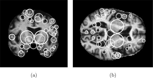
Illustrating scale-invariant features extracted in an MR volume. Circles represent the locations and scales of features in (a) a coronal slice and (b) an axial slice. Solid circles indicate features present in both slices, dashed circles indicate features present in a single slice. Note how feature scales reflect the spatial extent of the underlying anatomical structures, e.g. the width of sulci or ventricles. Here, features are extracted using the DOG operator (Lowe, 2004) and features shown are located within 2 voxels of the corresponding slice through in the 3D volume.

With regard to morphometric analysis, features extracted in a Gaussian scale-space are interesting for several reasons. Feature geometries reflect the locations and scales of natural anatomical structures in the image in a manner independent of image resolution, and analysis can avoid depending on arbitrary locations and scales determined by the particular imaging device used, e.g. using the entire image or single voxels. As features arise from derivatives or changes in image content, they typically correspond to distinctive image patterns whose presence or absence in an image can be established more readily than arbitrary image regions. Features are invariant to geometrical deformations including image translations, orientations and magnifications, and features corresponding to the same anatomical structures can thus be reliably extracted despite local tissue misalignments following initial coarse inter-subject or atlas-to-subject registration. Features are invariant to locally linear intensity changes, and the same anatomical structures can thus be robustly identified despite image intensity variations due to factors such as scanner non-uniformity, etc. Finally, features can be efficiently extracted in O(N log N) time and space complexity using image pyramid data representations (Lowe, 2004), where N is the size of the image in voxels.

2.2. Probabilistic Modeling of Features

While scale-invariant features can be robustly extracted despite intensity and geometrical changes, it is difficult to identify features arising from the same underlying tissue in different subjects. In general, such features vary in geometry and appearance from one subject to the next, and cannot be reliably extracted in all subjects, due to inter-subject and inter-group variability. The goal of probabilistic modeling is thus to identify features which do occur with statistical regularity in subsets of subjects, and to quantify their variability and informativeness with respect to subject groups.

Here, an individual feature is denoted as f_i = {a_i, α_i, g_i, γ_i}. a_i is a vector of image measurements representing the image appearance of a local feature. α_i is a binary random variable indicating whether a_i represents the appearance of a valid feature instance or random noise. g_i = {x_i, σ_i} represents the geometry of a feature in terms of image location x_i and scale σ_i. γ_i is a binary random variable indicating the presence or absence of geometry g_i in a subject image.

Let F = {f₁, . . . , f_N} represent a set of N local features extracted from a set of images, where N is unknown. Let T represent a geometrical transform bringing features into coarse, approximate alignment with an atlas, e.g. a rigid or affine transform to the Talairach space (Talairach and Tournoux, 1988). Let C represent a discrete random variable of the group from which subjects are sampled, e.g. diseased, healthy. The posterior probability of (C, T ) given F can be expressed as:

$$p(C,T\mid F)=\frac{p(C,T)p(F\mid C,T)}{p\left(F\right)}=\frac{p(C,T){\prod }_i^{N}p(f_i\mid C,T)}{p\left(F\right)},$$ (3)

where the first equality results from Bayes rule and the second from the assumption of conditional feature independence given (C, T ). The assumption of conditional independence is reasonable here, as inter-feature intensity dependencies are largely absent for features localized in scale and in space, and inter-feature geometrical dependencies are largely accounted for via knowledge of (T, C). To illustrate, consider the case of a pathology that tends to introduce a systematic bias into spatial normalization. Features f_j and f_j will generally exhibit bias-related dependencies, however variables (T, C) account for such dependencies, leaving f_j and f_j conditionally independent. In Equation (3), p(f_i|C, T) represents the probability of a feature f_i given (C, T), p(C, T) represents a joint prior distribution over (C, T) and p(F) represents the evidence of feature set F . The focus of modeling is on the conditional feature probability p(f_i|C, T) which is expressed as:

$$\begin{array}{cc}\hfill p(f_i\mid C,T)=& p(a_i,{\alpha }_i,g_i,{\gamma }_i\mid C,T),\hfill \\ \hfill =& p(a_i\mid {\alpha }_i,g_i,{\gamma }_i,C,T)p({\alpha }_i\mid g_i,{\gamma }_i,C,T)p(g_i\mid {\gamma }_i,C,T)p({\gamma }_i\mid C,T),\hfill \end{array}$$ (4)

$$=p(a_i\mid {\alpha }_i)p({\alpha }_i\mid {\gamma }_i)p(g_i\mid {\gamma }_i,T)p({\gamma }_i\mid C).$$ (5)

Here, Equation (4) follows from the chain rule of probability, and Equation (5) follows from several reasonable conditional independence assumptions between variables. Feature appearance a_i is conditionally independent of (g_i, γ_i, C, T) given α_i, and p(a_i|α_i) is a density over feature appearance a_i given appearance validity α_i. Appearance validity α_i is conditionally independent of (g_i, C, T) given the occurrence of a consistent geometry γ_i. p(α_i|γ_i) thus represents a Bernoulli distribution over α_i, as specified by γ_i = 0 and γ_i = 1. Feature geometry g_i is conditionally independent of C given geometrical occurrence γ_i and global transform T , and p(g_i|γ_i, T) is a density over g_i conditional on (γ_i, T). Finally, feature geometrical occurrence γ_i is conditionally independent of T given the group C, and p(γ_i|C) thus represents a Bernoulli distribution over γ_i for each subject group C.

2.2.1. Model Learning

Learning focuses on identifying clusters of features which are similar in terms of their group membership, geometry and appearance. Features in a single cluster represent different observations of the same underlying, group- related anatomical structure, and can be used to estimate the parameters of distributions in Equation (5). Figure 2 illustrates an example of features in different subjects grouped into a cluster during model learning.

Figure 2.

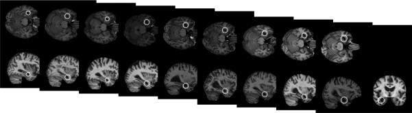
White circles represent features in different subjects which are similar in terms of their appearance, geometry and group membership. These features are considered to arise from the same underlying group-related anatomical structure and grouped into a single cluster in model learning. The features shown here are identified in 10 of 75 Alzheimer's subjects and in none of 75 normal control subjects.

Preprocessing

Subject images are first aligned into a global reference frame, and T is thus constant in Equation (3). At this point, images have been normalized according to location, scale and orientation, and the remaining appearance and geometrical variability of anatomical structure can be described (Dryden and Mardia, 1998). Image features are then detected independently in all subject images as in Equation (2).

Clustering

For each feature f_i, two different clusters or feature sets G_i and A_i are identified, where f_j ∈ G_i are similar to f_i in terms of geometry, and f_j ∈ A_i are similar to f_i in appearance. First, set G_i is identified based on a robust binary measure of geometrical similarity. Features f_i and f_j are said to be similar if their locations and scales differ by less than error thresholds ε_x and ε_σ. In order to compute geometrical similarity in a scale-independent manner, location difference is normalized by feature scale σ_i, and scale difference is computed in the log domain. G_i is thus defined for each f_i as:

$$G_i=\left\{f_j:\frac{\Vert x_i-x_j\Vert }{{\sigma }_i}\le {\epsilon }_x\wedge \mid \ln \frac{{\sigma }_j}{{\sigma }_i}\mid \le {\epsilon }_{\sigma }\right\},$$ (6)

Here, thresholds ε_x and ε_σ represent the maximum acceptable deviation in the location and scale of a feature across subjects within normalized Talairach space. These can be set empirically or determined automatically; larger values may result in grouping geometrically different anatomical structures within a single model feature and produce a smaller overall feature set, smaller values will result in treating variations of the same anatomical structure as unique features and produce a larger feature set. In general, these thresholds can be set generously, as feature appearance will play an important role in sorting out ambiguities.

Next, set A_i is identified using a robust measure of appearance similarity, where f_i is said to be similar to f_j in appearance if the difference between their appearances is below a threshold ε_ai. A_i is thus a function of ε_ai and defined for each f_i as:

$$A_i\left({\epsilon }_{a_i}\right)=\{f_j:\Vert a_i-a_j\Vert \le {\epsilon }_{a_i}\},$$ (7)

where in this paper, ∥ ∥ represents the Euclidean norm between appearance vectors a_i normalized to unit length, and reflects the assumption of independent and identically distributed image measurements in a_i and a_j. Note that while a single pair of geometrical thresholds (ε_x, ε_σ) applies to all features, ε_ai is feature-specific and an optimal value is automatically determined for each feature such that:

$${\epsilon }_{a_i}=\sup \left\{{\epsilon }_a\in [0,\infty ):1\le \frac{\mid G_i\cap C_i\cap A_i\left({\epsilon }_a\right)\mid }{\mid \overline{G_i\cap C_i}\cap A_i\left({\epsilon }_a\right)\mid }\right\},$$ (8)

where C_i is the group associated with feature f_i. ε_ai is thus set to reflect the maximum permissible discrepancy in appearance such that the features are still more likely than not to arise from the same geometrically consistent, group-related anatomical structure. An important practical detail is to ensure that the ratio in Equation (8) is well-defined in the presence of sparse data, e.g. when $\mid \overline{G_i\cap C_i}\cap A_i\left({\epsilon }_{a_i}\right)\mid =0$. This can be done by adding small artificial counts to both the numerator and denominator of the ratio, a procedure referred to as Dirichlet regularization (Bishop, 2006).

Reduction

The intersection $G_i\cap A_i$ represents a cluster of features which share a common geometry and appearance with f_i, and arise from the same underlying anatomical pattern. Since clusters (G_i, A_i) are generated for all images features f_i, many effectively correspond to the same feature cluster. A reduced set of model features is identified by discarding a set R of all features which are themselves elements of a larger cluster f_i:

$$R=\{f_j:f_j\in G_i\cap A_i\wedge \mid G_i\cap A_i\mid >\mid G_j\cap A_j\mid \}.$$ (9)

Reduction effectively compresses the set of raw features extracted in all subjects into a smaller, more meaningful set of model features, which represent probable inter-subject correspondences and can be used to quantify the relationship between anatomy and subject groups. Note that in general, a degree of partial overlap may exist between model features resulting from this reduction process, and more sophisticated feature reduction or clustering techniques could be potentially applied, e.g. structural group analysis (Coulon et al., 2000; Thirion et al., 2007). In the context of FBM, however, the distinctive appearance component of scale-invariant features aids significantly in disambiguating between different yet geometrically similar features, and partial overlap is rarely observed in practice.

2.2.2. Morphometric Analysis

The aim of FBM is to automatically discover group-related anatomical structures, which can be used in order to guide further investigation into the anatomical basis for group differences or as disease biomarkers. The informativeness of a feature regarding group is quantified by the following likelihood ratio:

$$\frac{p(f_i=1\mid C_i,T)}{p(f_i=1\mid \overline{C_i},T)}=\frac{\mid \{f_j:f_j\in G_i\cap C_i\cap A_i\}\mid }{\mid \{f_j:f_j\in G_i\cap \overline{C_i}\cap A_i\}\mid },$$ (10)

where f_i = 1 is used as shorthand here to signify the event of positive feature occurrence (α_i = 1, γ_i = 1). The ratio in Equation (10) represents the likelihood that f_i co-occurs with group C_i vs. another different group C̄_i. This ratio explicitly measures the degree of association between an image feature and a specific subject group, and lies at the heart of FBM analysis. Features can be sorted according to likelihood ratios to identify the anatomical structures most indicative of a particular subject group, e.g. healthy or diseased, and those with likelihood ratios near 1 can be disregarded as uninformative. As in Equation (8), Dirichlet regularization is applied to cope with sparse data when estimating the likelihood ratio.

The statistical significance of the relationship between an individual feature and subject groups can be expressed using Fisher's exact test, where p-values are calculated from a contingency table of feature/group co-occurrence frequencies. Techniques such as Bonferroni correction or permutation testing (Nichols and Holmes, 2001) can be used to correct p-values for multiple comparisons to control the probability of committing a type I error. In scenarios such as FBM where the goal is to discover group-related features amid a high number of potential candidates, Bonferroni-type correction procedures which express the probability of any error may be unnecessarily conservative. In particular, the probability that a certain fraction of apparently group-related features arise by random chance may be relatively high, however this does not preclude the possibility of discovering a significant number of valid group-related features. An appropriate alternative here is the false discovery rate (FDR) (Benjamini and Hochberg, 2001), defined as the fraction of features falling below an uncorrected p-value threshold which represent false rejections of the null hypothesis, i.e. that features are statistically unrelated to subject groups. The FDR can be calculated using the method of Benjamimi and Hochberg (Benjamini and Hochberg, 2001) for subsets of features f_i with the smallest uncorrected p-values.

2.2.3. Classifying New Subjects

The FBM framework can be used to identify group-related features in new subjects and to classify new subjects according to group, a procedure potentially useful for computer-aided diagnosis. Classification begins by first aligning a new subject image into stereotactic space via T and extracting image features, as in the learning procedure. A set of model features F is then identified in the new subject in a manner similar to model learning, where a model feature f_i is declared to be identified if an image feature f_j in the new subject exists such that $\Vert a_i-a_j\Vert \le {\epsilon }_{a_i},\frac{\Vert x_i-x_j\Vert }{{\sigma }_i}\le {\epsilon }_x\text{and}\mid \ln \frac{{\sigma }_j}{{\sigma }_i}\mid \le {\epsilon }_{\sigma }$. Classification based on identified features can then be expressed as:

$$C^{\ast }=\underset{C}{\mathrm{argmax}}\left\{\frac{p(C,T\mid F)}{p(\overline{C},T\mid F)}\right\}=\underset{C}{\mathrm{argmax}}\left\{\frac{p(C,T)}{p(\overline{C},T)}\prod _i\frac{p(f_i\mid C,T)}{p(f_i\mid \overline{C},T)}\right\},$$ (11)

where C* is the optimal Bayes classification. In Equation (11), classification is primarily driven by the data likelihood ratio ${\prod }_i\frac{p(f_i\mid C,T)}{p(f_i\mid \overline{C},T)}$ based on the link between individual model features and groups as in Equation (10). Factor $\frac{p(C,T)}{p(\overline{C},T)}$ represents the ratio of prior probabilities over subject group and transform. Note that thresholding the data likelihood ratio at 1 is generally ineffective for classification, as different subject groups generally occur with different frequencies in training and testing data, and produce different numbers of group-informative features. Instead, the prior probability ratio can be varied in order to balance the sensitivity/specificity rates of classification in a clinical setting.

3. Materials and Methods

FBM is a general technique that can be used to discover group-related anatomical structure in volumetric image sets. In order to validate FBM, we choose the example application of Alzheimer's disease (AD) analysis, as AD is a well-known, important, incurable neurodegenerative disease affecting millions worldwide, and is the focus of intense computational research (Qiu et al., 2009; Kloppel et al., 2008; Duchesne et al., 2008; Marcus et al., 2007; Buckner et al., 2004).

Experiments use OASIS (Marcus et al., 2007), a large, freely available data set including 98 normal (NC) subjects and 100 probable AD subjects ranging clinically from very mild to moderate dementia. All subjects are right-handed, with approximately equal age distributions for NC/AD subjects ranging from 60+ years with means of 76/77 years. For each subject, 3 to 4 T1-weighted scans are acquired, gain-field corrected and averaged in order to improve the signal/noise ratio. Images are aligned within the Talairach reference frame via affine transform T and the skull is masked out (Buckner et al., 2004).

The DOG scale-space (Lowe, 2004) is used to identify feature geometries (x_i, σ_i). Feature appearances a_i are obtained by cropping cubical image regions of side length $4\sqrt{{\sigma }_i}$ centered on x_i, which are then scaled to (11×11×11)-voxel resolution. Voxel intensities are shifted to zero mean and normalized to unit length. Rotation invariance can also be achieved (Allaire et al., 2008), however this is omitted here as subjects are already rotation-normalized via T and further invariance reduces appearance distinctiveness. Spurious features will naturally arise from anatomical structure such as surfaces or tissue boundaries, which cannot be reliably localized in all spatial directions. These can be identified and discarded via an analysis of the 3 × 3 Hessian matrix H, calculated from derivatives of image intensity with respect to spatial coordinates about feature location and scale. Features for which the ratio $\frac{Det\left(H\right)}{T{r}^3\left(H\right)}$ of the determinant vs. the cubed trace of H is low indicate degenerate patterns whose localization within the image is under-determined, and a threshold can be imposed based on this ratio to discard such features (Lowe, 2004). Approximately 800 features are extracted in each (176 × 208 × 176)-voxel brain volume.

For model learning, geometrical error threshold values used are empirically set to ${\epsilon }_x=\frac{{\sigma }_i}{2}$ and ${\epsilon }_{\sigma }=\ln \frac{3}{2}$, these values are chosen generously in an attempt to include the natural range of variation of features across different subjects in normalized Talairach space. Further increasing these values increases the tendency to group geometrically similar yet different anatomical patterns into the same geometrical clusters, however the net effect on the set of model features resulting from learning is minimal, as ambiguities in geometrical clustering are resolved in a consistent manner in the subsequent stage of appearance clustering. Significantly decreasing these values, however, tends to fragment model features, as the maximum permissible geometrical variability is insufficient for effectively clustering features arising from the same underlying anatomical structure.

4. Results

To investigate discovery of group-related anatomical patterns, model learning is applied on a randomly-selected subset of 150 subjects (75 NC, 75 AD). Approximately 12K model features are identified via the learning processes, these are graphed in Figure 3. The solid curve in Figure 3 plots the occurrence frequency p(f_i = 1|T) of features in the training set, which is proportional to the sizes of feature clusters identified during learning. Note that a large number of features occur infrequently and are observed in few subjects. In general the number of subject images required to obtain a good sampling is feature-specific and related to the intrinsic feature occurrence frequencies; frequently occurring features can be repeatably observed and modeled from few subject images, while features arising from more subtle anatomical structure can only be observed in larger data sets.

Figure 3.

The dashed curve plots the likelihood ratio $\ln \frac{p(f_i=1\mid AD,T)}{p(f_i=1\mid NC,T)}$ of feature occurrence in AD vs. NC subjects sorted in ascending order, low values indicate features associated with NC subjects (lower left) and high values indicate features associated with AD subjects (upper right). The solid curve plots feature occurrence probability p(f_i = 1|T), which is proportional to the cardinality of model feature clusters identified during learning. Note a large number of frequently-occurring features bear little information regarding AD or NC (center of graph). Examples of highly NC-related (1-3) and AD-related (a-c) features are shown, along with their associated likelihood ratios.

The dashed curve in Figure 3 plots the likelihood ratio of feature occurrence in AD vs. NC subjects, along with several examples of AD- and NC-related features. A number of features identified occur frequently, yet bear little information regarding subject group (center of graph). A signifi-cant number are strongly indicative of either NC or AD subjects (extreme left or right of graph). Furthermore, the locations and scales of many strongly group-related features are consistent with brain regions known to differ between AD and NC groups, and their appearances can be interpreted in terms of established indicators of AD in the brain. For examples of AD-related features shown in Figure 3, feature (a) corresponds to enlargement of the extracerebral space in the anterior Sylvian sulcus; feature (b) corresponds to enlargement of the temporal horn of the lateral ventricle (and one would assume a concomitant atrophy of the hippocampus and amygdala); feature (c) corresponds to enlargement of the lateral ventricles. For NC-related features, features (1) (parietal lobe white matter) and (2) (posterior cingulate gyrus) correspond to non-atrophied parenchyma and feature (3) (lateral ventricle) to non-enlarged cerebrospinal fluid spaces.

Examples of the 8 most statistically significant AD-related and NC-related features are shown in Figures 4 and 5. In Figure 4, six of the eight most significant AD-related features correspond to established indicators of AD, independently identified in both hemispheres. Specifically, (a-l, a-r) represent the anterior poles of the enlarged lateral ventricles, (b-l, b-r) represent regions of atrophied white matter and (c-l, c-r) represent the enlarged temporal poles of the lateral ventricles. (d) represents the enlargement of the extracerebral space in the anterior Sylvian sulcus and (e) represents the enlargement of the posterior region of the right lateral ventricle. Figure 5 illustrates the eight most significant features associated with NC subjects. The 16 features in Figures 4 and 5 fall within the set of the 25 most significant group-related features, associated with a false discovery rate of 0.15. For these 25 features, 21-22 could thus be expected to result from valid group-related image structure. Note that traditional morphometry methods can be used to identify differences in similar brain regions, for example the 2-sample t-test approach used in VBM shows differences between AD/NC groups in regions similar to Figure 4 (c-l, c-r) (Whitwell et al., 2007). Although traditional methods can identify regions in which voxel-level group differences occur, questions may remain as to the nature of these differences: are they due to systematic group-related differences in spatial normalization (Bookstein, 2001)? Are they the result of multiple, distinct patterns of anatomy present in the region in different subjects? FBM focuses on identifying distinctive image features, that need not be present in all subjects and that tend to occur preferentially in subjects of similar groups, thereby providing a framework for addressing such questions.

Figure 4.

Examples of the eight most significant AD-related features, shown in sagittal and coronal slices. The feature occurrence frequencies within 75 AD and 75 NC subjects and associated uncorrected p-values are given. Out of eight features, six represent similar anatomical regions identified independently in left and right hemispheres. All represent neuroanatomical regions known to be affected by AD.

Figure 5.

Examples of the eight most significant NC-related features, shown in sagittal and coronal slices. The feature occurrence frequencies within 75 AD and 75 NC subjects and associated uncorrected p-values are given. Most features lie near the mid-sagittal plane (1-6), and reflect stable un-atrophied cortical (1-3) or sub-cortical (4-6) structure. Feature (7) represents an anatomical pattern reflective of natural age-related atrophy, feature (8) represents a distinctive cortical fold.

FBM can also be used to classify new subjects in a computer-aided diagnosis scenario. An analysis of classification performance must take into account the clinical and demographic information of the experimental subjects, and the degree of AD-specific prior information incorporated into classification. In terms of demographic/clinical information, AD subjects exhibiting very mild dementia (i.e. bearing a clinical dementia rating (CDR) of 0.5) are more difficult to discriminate from healthy subjects than those exhibiting mild or moderate dementia (i.e. CDR=1 or 2), and several approaches restrict classification to mild AD (Kloppel et al., 2008; Duchesne et al., 2008). Furthermore, elderly subjects are more easily confused with AD subjects due to the appearance of normal age-related atrophy, and imposing age limits generally improves classification (Kloppel et al., 2008). In terms of prior information, classification can generally be improved by focusing on specific measurements or regions of interest (ROIs) known to be implicated in AD, e.g. pre-segmented grey matter maps (Kloppel et al., 2008) or the medial temporal lobe region (Kloppel et al., 2008; Duchesne et al., 2008). Classification rates as high as 0.92 have been achieved using the classic support vector machine (SVM) method (Cortes and Vapnik, 1995) on intensity data in the medial temporal lobe region (Duchesne et al., 2008), and perfect classification has been achieved from measurements such as the entorhinal cortex thickness and the hippocampus volume (Desikan et al., 2009).

Classification here is performed in a leave-one-out manner, where each OASIS test subject in turn is kept aside and classified using an FBM model trained on all other subjects. Note that the training subjects and thus the learned model features vary from one trial to the next, however by inspection the most significant group-related model features are consistently identified across trials, e.g. those shown in Figures 4 and 5. While FBM model learning makes use of all 198 OASIS subjects (minus the test subject), classification results are reported on 3 different divisions of test subjects, in order to illustrate the effect of age and the severity of clinical diagnosis on classification performance:

1. Subjects aged 60-80 years, mild AD (CDR=1) (66 NC, 20 AD), a scenario similar to (Kloppel et al., 2008).

2. Subjects aged 60-96 years, mild AD (CDR=1) (98 NC, 28 AD), to illustrate classification of elderly subjects.

3. Subjects aged 60-80 years, both mild and very mild AD (CDR=1 and 0.5) (66 NC, 69 AD), to illustrate classification of very mild AD.

The receiver operating characteristic (ROC) curves these three divisions are plotted in Figure 6. Division 1) results in an equal error classification rate (EER) ³ of 0.80. A slightly higher classification rate of 0.81 is reported in a similar scenario using the SVM-based method (Kloppel et al., 2008), although a direct comparison cannot be drawn as the underlying data sets are different, and AD severity categories are defined differently. In (Kloppel et al., 2008) for instance, mild AD is defined by Mini Mental State Examination (MMSE) score ≥ 20 with mean MMSE = 23.5, and in OASIS (Marcus et al., 2007) by CDR=1, with corresponding mean MMSE = 20.8, stdev = 3.7. Note also that the work of (Kloppel et al., 2008) makes use of AD-related measurements in the form of grey matter maps, while FBM operates on features extracted throughout the brain and subcortical regions. For divisions 2) and 3), classification rates drop to EER = 0.70 and 0.71, respectively, demonstrating the difficulty in classifying subjects that are elderly or exhibit very mild AD. A rate of EER = 0.65 is obtained for leave-one-out trials on all 198 OASIS subjects, where classification errors are largely due to younger subjects with very mild AD and elderly NC subjects.

Figure 6.

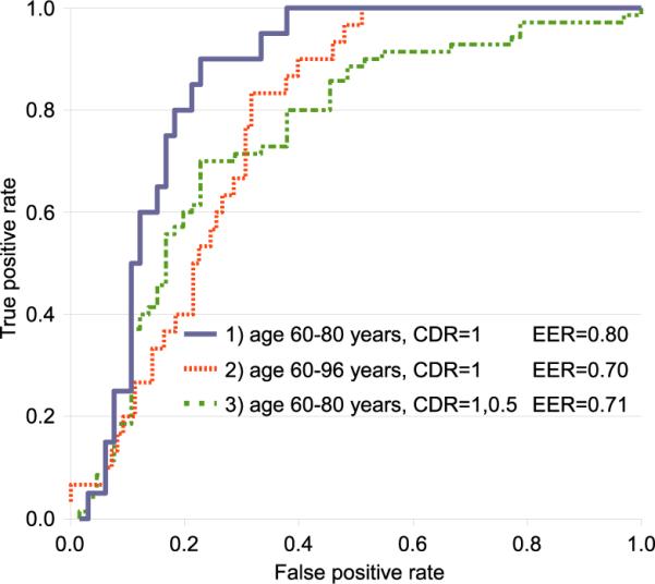
ROC curves for leave-one-out classification divisions. Maximum classification accuracy is achieved in 1) for subjects with mild AD (CDR=1) and within 60-80 years of age (solid curve, EER = 0.80). Including 2) elderly subjects or 3) very mild AD cases both result in reduced classification performance.

To our knowledge, classification results have not yet been reported on the OASIS data in a comparable image-based classification scenario, and we attempted a baseline image-based classification experiment using the popular SVM method, see details in Appendix A. Classification was unsuccessful despite investigating various combinations of SVM kernels and image preprocessing steps, speaking to the difficulty of image-based classification. Note that while affine-aligned OASIS subject images are used here, more effective SVM classification of AD/NC subjects has been reported using deformable image alignment (Lao et al., 2004; Duchesne et al., 2008). While SVMs are useful for classification, they require additional interpretation to explain the link between anatomical tissues and groups (Lao et al., 2004). The primary advantage of FBM is the ability to automatically identify distinctive, group-related anatomical patterns that may not be present in all subjects, in addition to the ability to classify new subjects.

5. Discussion

This paper presents and validates feature-based morphometry (FBM), a new, fully data-driven technique for discovering group-related anatomical structures in volumetric images. The primary difference between FBM and other morphological analysis techniques is that FBM explicitly addresses the situation where one-to-one inter-subject correspondence does not exist between all subjects, due to disease or anatomical variability. This is achieved by modeling the image as a collage of local scale-invariant features that need not occur in all subjects, which provides a mechanism to avoid confounding analysis of tissues which may not be present or easily localizable in all subjects. FBM is based on learning a probabilistic model of local, scale-invariant features which reflect group-related anatomical characteristics. A clinical validation is performed on a set of 198 NC and probable AD subjects from the large, freely available OASIS data set (Marcus et al., 2007). Anatomical features consistent with established differences between NC and AD brains are automatically discovered in a set of 150 training subjects. The significance of features identified is quantified in terms of the false discovery rate (FDR), and analysis shows that a sizable set of group-related features can be identified with a low FDR. FBM is potentially useful for computer-aided diagnosis, and leave-one-out trials achieve a classification rate of EER = 0.80 for subjects aged 60-80 years exhibiting mild AD (CDR=1) in a scenario similar to recent work (Kloppel et al., 2008). To our knowledge, classification results for similar methods where measurements or regions of interest are not known a priori have not yet been published for the OASIS data set, however the OASIS data set is freely available and comparison with other techniques in the literature will be possible.

FBM does not replace current morphometry techniques, but rather provides a complementary approach which is particularly useful in the situation where one-to-one inter-subject correspondence is ambiguous or difficult to achieve. For this reason, FBM has the potential to become widely used in contexts such as neurological disease analysis, where this is often the case. The work here considers group differences in terms of feature/group co-occurrence statistics, however most features do occur (albeit at different frequencies) in multiple groups, and traditional morphometric analysis on an individual feature basis is a logical next step in further characterizing group differences. In terms of FBM theory, the model could be adapted to account for disease progression in longitudinal studies, to aid in understanding the neuroanatomical basis for progression from mild cognitive impairment to AD for instance. Thresholds on permissible geometrical error ε_x and ε_σ are currently fixed to reasonable empirical values. Experimentally, the same significant group-related model features are consistently identified using larger thresholds (e.g. ε_x = 1.0, ε_σ = ln 1.8), however they tend to become fragmented for lower thresholds (e.g. below ε_x = 0.4, ε_σ = ln 1.4). Optimal values could potentially be estimated automatically from data, and it is possible that spatially varying threshold may offer improved modeling, e.g. allowing for greater geometrical variability in the cortex. Many different types of scale-invariant features other than DOG features have been developed, these could be incorporated into FBM to discover a greater variety of group-related anatomical patterns and to improve classification. Finally, a future experiment will be to assess the repeatability of features identified in different FBM models trained on independent image sets, this will require a principled means of comparing sets of model features derived from different data sets.

A. Details of SVM Experiments

SVM classification trials were performed on random training/testing set divisions of the OASIS data, with images preprocessed using Gaussian-smoothing with blurring kernels of standard deviation (0, 1, 2, 4 voxels). RBF and Linear SVM kernels were tested. The Linear SVM kernel is defined by a single parameter C relating to the error margin, the RBF kernel is defined by parameters C (as in the Linear kernel) and γ which controls the width of the kernel. Exhaustive searches were performed in order to determine optimal parameter values. Classification was unsuccessful; the SVM was not capable of learning a viable decision boundary and in all trials defaulted to guessing the most frequent group label in the training set. A maximum classification rate of ≈ 0.5 was thus obtained here for approximately equal numbers of AD and NC test subjects.

References

- Allaire S, Kim J, Breen S, Jaffray D, Pekar V. Full orientation invariance and improved feature selectivity of 3d sift with application to medical image analysis. IEEE Workshop on Mathematical Methods in Biomedical Image Analysis. 2008 [Google Scholar]
- Ashburner J, Friston KJ. Voxel-based morphometry-the methods. NeuroImage. 2000;11(23):805–821. doi: 10.1006/nimg.2000.0582. [DOI] [PubMed] [Google Scholar]
- Ashburner J, Friston KJ. Comments and controversies: Why voxel-based morphometry should be used. NeuroImage. 2001;14:1238–1243. doi: 10.1006/nimg.2001.0961. [DOI] [PubMed] [Google Scholar]
- Ashburner J, Hutton C, Frackowiak R, Johnsrude I, Price C, Friston K. Identifying global anatomical differences: deformation-based morphometry. Human Brain Mapping. 1998;6(6):348–357. doi: 10.1002/(SICI)1097-0193(1998)6:5/6<348::AID-HBM4>3.0.CO;2-P. [DOI] [PMC free article] [PubMed] [Google Scholar]
- Bajcsy R, Kovacic S. Multiresolution elastic matching. Computer Vision, Graphics and Image Processing. 1989;46:1–21. [Google Scholar]
- Baloch S, Verma R, Davatzikos C. An anatomical equivalence class based joint transformation-residual descriptor for morphological analysis. Intl. Conf. on Information Processing in Medical Imaging. 2007 doi: 10.1007/978-3-540-73273-0_49. [DOI] [PubMed] [Google Scholar]
- Benjamini Y, Hochberg Y. The control of the false discovery rate in multiple testing under dependency. Ann. Stat. 2001;29:1165–1188. [Google Scholar]
- Bishop CM. Pattern Recognition and Machine Learning. Springer; 2006. [Google Scholar]
- Blezek DJ, Miller JV. Atlas stratification. Intl. Conf. on Medical Image Computing and Computer Assisted Intervention. 2006 doi: 10.1007/11866565_87. [DOI] [PubMed] [Google Scholar]
- Bookstein F. Principle warps: thin-plate splines and the decomposition of deformations. IEEE Trans. on Pattern Analysis and Machine Intelligence. 1989;11(6):567–585. [Google Scholar]
- Bookstein FL. voxel-based morphometry should not be used with imperfectly registered images. NeuroImage. 2001;14:1454–1462. doi: 10.1006/nimg.2001.0770. [DOI] [PubMed] [Google Scholar]
- Bro-Nielsen M, Gramkow C. Fast fluid registration of medical images. Visualization in Biomedical Computing. 1996:267–276. [Google Scholar]
- Buckner R, Head D, Parker J, Fotenos A, Marcus D, Morris J, Snyder A. A unified approach for morphometric and functional data analysis in young, old, and demented adults using automated atlas-based head size normalization: reliability and validation against manual measurement of total intracranial volume. Neuroimage. 2004;23:724–38. doi: 10.1016/j.neuroimage.2004.06.018. [DOI] [PubMed] [Google Scholar]
- Carneiro G, Jepson A. Multi-scale phase-based local features. IEEE Conf. on Computer Vision and Pattern Recognition. 2003;1:736–743. [Google Scholar]
- Cheung W, Hamarneh G. N-sift: N-dimensional scale invariant feature transform for matching medical images. IEEE Intl. Symp. on Biomedical Imaging. 2007 doi: 10.1109/TIP.2009.2024578. [DOI] [PubMed] [Google Scholar]
- Chung MK, Worsley KJ, Paus T, Cherif C, Collins DL, Giedd JN, Rapoport JL, Evans AC. A unified statistical approach to deformation-based morphometry. Neuroimage. 2001;14:595–606. doi: 10.1006/nimg.2001.0862. [DOI] [PubMed] [Google Scholar]
- Cortes C, Vapnik V. Support-vector networks. Machine Learning. 1995;20(3):273–297. [Google Scholar]
- Coulon O, Mangin J, Poline J, Zilbovicius M, Roumenov D, Samson Y, Frouin V, Bloch I. Structural group analysis of functional activation maps. NeuroImage. 2000;11:767–782. doi: 10.1006/nimg.2000.0580. [DOI] [PubMed] [Google Scholar]
- Davatzikos C. Comments and controversies: Why voxel-based morphometric analysis should be used with great caution when characterizing group differences. NeuroImage. 2004;23:17–20. doi: 10.1016/j.neuroimage.2004.05.010. [DOI] [PubMed] [Google Scholar]
- Desikan RS, Cabral HJ, Hess CP, Dillon WP, Glastonbury CM, Weiner MW, Schmansky NJ, Greve DN, Salat DH, Buckner RL, Fischl B, Initiative ADN. Automated mri measures identify individuals with mild cognitive impairment and alzheimer's disease. Brain: 2009. In Press. [DOI] [PMC free article] [PubMed] [Google Scholar]
- Dryden IL, Mardia KV. Statistical Shape Analysis. John Wiley & Sons; 1998. [Google Scholar]
- Duchesne S, Caroli A, Geroldi C, Barillot C, Frisoni GB, Collins DL. Mri-based automated computer classification of probable ad versus normal controls. IEEE Trans. on Medical Imaging. 2008;27:509–520. doi: 10.1109/TMI.2007.908685. [DOI] [PubMed] [Google Scholar]
- Fan Y, Shen D, Gur RC, Gur RE, Davatzikos C. Compare: Classification of morphological patterns using adaptive regional elements. IEEE Trans. on Medical Imaging. 2007;26(1):94–105. doi: 10.1109/TMI.2006.886812. [DOI] [PubMed] [Google Scholar]
- Fergus R, Perona P, Zisserman A. Weakly supervised scale-invariant learning of models for visual recognition. Intl. J. of Computer Vision. 2006;71(3):273–303. [Google Scholar]
- Harris C, Stephens M. A combined corner and edge detector. Proceedings of the 4th Alvey Vision Conference. 1988:147–151. [Google Scholar]
- Hellier P, Barillot C, Corouge I, Gibaud B, Le Goualher G, Collins D, Evans A, Malandain G, Ayache N, Christensen G, Johnson H. Retrospective evaluation of intersubject brain registration. IEEE Trans. on Medical Imaging. 2003 Sep;22(9):1120–1130. doi: 10.1109/TMI.2003.816961. [DOI] [PubMed] [Google Scholar]
- Kadir T, Brady M. Saliency, scale and image description. Intl. J. of Computer Vision. 2001;45(2):83–105. [Google Scholar]
- Kendall DG. A survey of the statistical theory of shape. Statistical Science. 1989;4(2):87–120. [Google Scholar]
- Klein A, Andersson J, Ardekani BA, Ashburner J, Avants B, Chiang M-C, Christensen GE, Collins DL, Gee J, Hellier P, Song JH, Jenkinson M, Lepage C, Rueckert D, Thompson P, Vercauteren T, Woods RP, Mann JJ, Parsey RV. Evaluation of 14 nonlinear deformation algorithms applied to human brain mri registration. NeuroImage. 2009 doi: 10.1016/j.neuroimage.2008.12.037. In Press. [DOI] [PMC free article] [PubMed] [Google Scholar]
- Klein A, Hirsch J. Mindboggle: A scatterbrained approach to automate brain labeling. NeuroImage. 2005;24:261–280. doi: 10.1016/j.neuroimage.2004.09.016. [DOI] [PubMed] [Google Scholar]
- Kloppel S, Stonnington CM, Chu C, Draganski B, Scahill RI, Rohrer JD, Fox NC, Jack CR, Jr, Ashburner J, Frackowiak RSJ. Automatic classification of mr scans in alzheimer's disease. Brain. 2008;131:681–689. doi: 10.1093/brain/awm319. [DOI] [PMC free article] [PubMed] [Google Scholar]
- Koenderink J. The structure of images. Biological Cybernetics. 1984;50:363–370. doi: 10.1007/BF00336961. [DOI] [PubMed] [Google Scholar]
- Lao Z, Shen D, Xue Z, Karacali B, Resnick SM, Davatzikos C. Morphological classification of brains via high-dimentional shape transformations and machine learning methods. NeuroImage. 2004;21:46–57. doi: 10.1016/j.neuroimage.2003.09.027. [DOI] [PubMed] [Google Scholar]
- Lindeberg T. Feature detection with automatic scale selection. Intl. J. of Computer Vision. 1998;30(2):79–116. [Google Scholar]
- Lindeberg T, Lidberg P, Roland PE. Analysis of brain activation patterns using a 3-d scale-space primal sketch. Human Brain Mapping. 1999;7:166–194. doi: 10.1002/(SICI)1097-0193(1999)7:3<166::AID-HBM3>3.0.CO;2-I. [DOI] [PMC free article] [PubMed] [Google Scholar]
- Lowe DG. Distinctive image features from scale-invariant keypoints. Intl. J. of Computer Vision. 2004;60(2):91–110. [Google Scholar]
- Mangin J, Riviere D, Cachia A, Duchesnay E, Cointepas Y, Papadopoulos-Orfanos D, Collins DL, Evans AC, Regis J. Object-based morphometry of the cerebral cortex. IEEE Trans. on Medical Imaging. 2004;23(8):968–983. doi: 10.1109/TMI.2004.831204. [DOI] [PubMed] [Google Scholar]
- Marcus D, Wang T, Parker J, Csernansky J, Morris J, Buckner R. Open access series of imaging studies (oasis): Cross-sectional mri data in young, middle aged, nondemented and demented older adults. Journal of Cognitive Neuroscience. 2007;19:1498–1507. doi: 10.1162/jocn.2007.19.9.1498. [DOI] [PubMed] [Google Scholar]
- Mikolajczyk K, Schmid C. Scale and affine invariant interest point detectors. Intl. J. of Computer Vision. 2004;60(1):63–86. [Google Scholar]
- Nichols TE, Holmes AP. Nonparametric permutation tests for functional neuroimaging: A primer with examples. Human Brain Mapping. 2001;15:1–25. doi: 10.1002/hbm.1058. [DOI] [PMC free article] [PubMed] [Google Scholar]
- Ono M, Kubik S, Abernathy CD. Atlas of the Cerebral Sulci. Thieme Medical; New York: 1990. [Google Scholar]
- Pohl K, Sabuncu M. A unified framework for mr based disease classification. Intl. Conf. on Information Processing in Medical Imaging. 2009 doi: 10.1007/978-3-642-02498-6_25. [DOI] [PMC free article] [PubMed] [Google Scholar]
- Qiu A, Fennema-Notestine C, Dale AM, Miller MI, Initiative ADN. Regional shape abnormalities in mild cognitive impairment and alzheimer's disease. NeuroImage. 2009;45:656–661. doi: 10.1016/j.neuroimage.2009.01.013. [DOI] [PMC free article] [PubMed] [Google Scholar]
- Rohr K. On 3D differential operators for detecting point landmarks. Image and Vision Computing. 1997;15(3):219–233. [Google Scholar]
- Sabuncu MR, Balci SK, Shenton ME, Golland P. Discovering modes of an image population through mixture modeling. IEEE Trans. on Medical Imaging. doi: 10.1007/978-3-540-85990-1_46. In Press. [DOI] [PMC free article] [PubMed] [Google Scholar]
- Studholme C, Drapaca C, Iordanova B, Cardenas V. Deformation-based mapping of volume change from serial brain mri in the presence of local tissue contrast change. IEEE Trans. on Medical Imaging. 2006;25(5):626–639. doi: 10.1109/TMI.2006.872745. [DOI] [PubMed] [Google Scholar]
- Sun ZY, Riviere D, Duchesnay E, Thirion B, Poupon F, Mangin J-F. Defining cortical sulcus patterns using partial clustering based on bootstrap and bagging. IEEE Intl. Symp. on Biomedical Imaging. 2008:1629–1632. [Google Scholar]
- Sun ZY, Riviere D, Poupon F, Regis J, Mangin J-F. Automatic inference of sulcus patterns using 3d moment invariants. Intl. Conf. on Medical Image Computing and Computer Assisted Intervention. 2007:515–522. doi: 10.1007/978-3-540-75757-3_63. [DOI] [PubMed] [Google Scholar]
- Talairach J, Tournoux P. Co-planar Stereotactic Atlas of the Human Brain: 3-Dimensional Proportional System: an Approach to Cerebral Imaging. Georg Thieme Verlag; Stuttgart: 1988. [Google Scholar]
- Thirion B, Pinel P, Tucholka A, Roche A, Ciuciu P, Mangin J-F, Poline J-B. Structural analysis of fmri data revisited: Improving the sensitivity and reliability of fmri group studies. IEEE Trans. on Medical Imaging. 2007;26(9):1256–1269. doi: 10.1109/TMI.2007.903226. [DOI] [PubMed] [Google Scholar]
- Thompson PM, Giedd JN, Woods RP, MacDonald D, Evans AC, Toga AW. Growth patterns in the developing human brain detected using continuum-mechanical tensor mapping. Nature. 2000;404(6774):190–193. doi: 10.1038/35004593. [DOI] [PubMed] [Google Scholar]
- Toews M, Arbel T. A statistical parts-based appearance model of anatomical variability. IEEE Trans. on Medical Imaging. 2007;26(4):497–508. doi: 10.1109/TMI.2007.892510. [DOI] [PubMed] [Google Scholar]
- Toews M, Collins DL, Arbel T. Automatically learning cortical folding patterns. IEEE Intl. Symp. on Biomedical Imaging. 2009:1330–1333. [Google Scholar]
- Toga AW, Thompson PM, Mega MS, Narr KL, Blanton RE. Probabilistic approaches for atlasing normal and disease-specific brain variability. Anat. Embryol. 2001;204:267–282. doi: 10.1007/s004290100198. [DOI] [PubMed] [Google Scholar]
- Whitwell JL, Przybelski SA, Weigand SD, Knopman DS, Boeve BF, Petersen RC, Jack CR., Jr 3d maps from multiple mri illustrate changing atrophy patterns as subjects progress from mild cognitive impairment to alzheimers disease. Brain. 2007;130:1777–1786. doi: 10.1093/brain/awm112. [DOI] [PMC free article] [PubMed] [Google Scholar]
- Witkin AP. Scale-space filtering. Int. Joint Conf. on Artificial Intelligence. 1983:1019–1021. [Google Scholar]
- Young RA. The gaussian derivative model for spatial vision: I. retinal mechanisms. Spatial Vision. 1987;2:273–293. doi: 10.1163/156856887x00222. [DOI] [PubMed] [Google Scholar]