Standardization of Relative Cerebral Blood Volume (rCBV) Image Maps for Ease of Both Inter- and Intrapatient Comparisons

Abstract

Relative cerebral blood volume (rCBV) measured using dynamic susceptibility contrast MRI suffers from interpatient and interstudy variability for the same tissue type. Traditionally, when a more quantitative assessment of rCBV is required, as for comparison across studies and patients, the rCBV values are normalized to the rCBV in a reference region such as normal-appearing white matter. However, this technique of normalization is subjective and time consuming and introduces user-dependent variability. In this study, we demonstrate that a method called standardization, applied to rCBV maps, is an objective means of translating all rCBV values to a consistent scale. This approach reduces interpatient and interstudy variability for the same tissue type, thus enabling easy and accurate visual and quantitative comparison across studies. One caveat to this approach is that it is not appropriate for the evaluation of global changes in blood volume, since systematic differences are removed in the process of standardization.

Dynamic susceptibility contrast MRI has demonstrated the potential to evaluate functional changes in cerebral blood volume (CBV) caused by brain tumor angiogenesis, providing a wealth of clinically relevant information (1–10). The standard approach is to collect T₂- or $T_2^{\ast }$-weighted images during the bolus administration of a gadolinium-chelated contrast agent. Using tracer kinetic principles, the resultant transient signal decrease is converted into a concentration-time curve, from which CBV is computed for each image pixel, thus providing a CBV image map. Since the arterial input function is often not measured, these maps show relative CBV values and are therefore usually termed rCBV maps.

One of the main limitations faced in using nonquantitative rCBV measurements to evaluate primary brain tumors is that the rCBV values for the same tissue type such as white matter, gray matter, or tumor can vary significantly across studies. This is true even for rCBV data obtained on the same scanner for the same patient using the same protocol. Consequently, in order to compare rCBV studies over time, even for the same patients, the rCBV values are typically normalized to a reference region such as normal-appearing white matter or contra-lateral reference brain. However, outlining regions of interest (ROI) for normalizing rCBV values is subjective in nature, thereby introducing variability. Also, the approach of normalization is very time consuming and therefore unlikely to become part of the routine clinical evaluation of longitudinal studies.

As a solution, we investigated the application of a standardization method for rCBV image maps. Previously, Nyul and Udupa (11,12) described the standardization technique for use in anatomic pre- and postcontrast images. They demonstrated that the standardized image intensities had a more consistent range and meaning for a given tissue type than the originals, that fixed gray-level windows could be established for the standardized images without the need for a per-case window level adjustment, and that standardization improved the degree of automation for image segmentation. In a previous preliminary study, Jensen and Schmainda (13) applied standardization to rCBV maps to demonstrate the potential for better discrimination of normal tissue types.

In this study, we develop the abovementioned standardization technique for rCBV maps. We validate the standardization routine by testing the hypothesis that standardization of rCBV maps accurately translates rCBV intensity values to a scale standard over tissue types, scanners, and subjects without corrupting the informational content of the processed maps. Finally, we demonstrate that standardized rCBV (STD rCBV) maps are superior to standard, or normalized, maps for comparison of studies across time.

THEORY

Since the basic theory and development of standardization has been described in detail elsewhere (11,12,14), it will be only briefly reviewed here, with the added focus being on a new application for the processing of rCBV maps.

Standardization is a two-step postprocessing method (Fig. 1) that standardizes the image intensity scale in such a way that for the same MR protocol and body region, similar intensities will have similar tissue meaning. For our purposes, this means that the same tissue type should have the same intensity, given in arbitrary units for all studies. In the first (training) step, a set of image maps is given as input. The parameters of a histogram transformation are learned from these data. Briefly, for each input data set within a training set, a histogram is created and the intensity value (ρ,) at several landmarks is determined. Landmarks are selected to be at the predefined percentiles of the histogram. Then, the intensity values between the first and last landmark (corresponding to the lowest and highest percentiles) are linearly mapped to the standardized scale with predefined minimum (s₁) and maximum (s₂) values. Next the corresponding standardized landmark (ρ′) for each input data set is calculated from the linear mapping. Finally, the rounded mean of all standardized landmarks (ρ₁....ρ₁₀) is used to find the standardized modes, μ,. This training step needs to be executed only once for a given protocol and body region.

FIG. 1.

The two-step method of standardization. Standardization is a two-step postprocessing method consisting of a training step and transformation step. Step 1, which is performed just once, is depicted at left, showing predefined upper and lower limits (s1, s2), landmarks (L_k) selected at predefined percentiles of each histogram, and intensity values determined at each landmark. The rounded mean of the intensity values determined for each input data set at each landmark is used to find the standardized modes, μ,. In the second (transformation) step, an input image is transformed using the parameters learned in the first step. Again, the histogram of the input image is calculated, and using the intensity values at the landmark percentile points, separate linear mappings are calculated to transform the input intensity values to the standardized values between each pair of landmarks. Example pre- and poststandardized T₁-weighted images are shown at the far right of the figure.

In the second (transformation) step, an input image, which may or not be part of the training set, is transformed using the parameters learned in the first step. This transformation is dependent on each individual image and therefore needs to be applied separately for each image. Again, the histogram of the input image is calculated, and using the intensity values at the landmark percentile points, separate linear mappings are calculated to transform the input intensity values to the standardized values between each pair of landmarks.

MATERIALS AND METHODS

Patient Population

All patients studied gave informed written consent under Health Insurance Portability and Accountability Act (HIPAA)-compliant guidelines approved by the institutional review board at our institution. Tumors were classified and graded according to the World Health Organization 1993 classification (15). The patient information, including age, gender, and tumor diagnosis, is provided in Table 1. A total of 26 patients with confirmed diagnosis of glioma were included in the study. The patient group was composed of 15 men and 11 women, ranging in age from 29–65 years. Of these 26 patients, 18 were used to generate the training file, five to test the algorithm, and another three to demonstrate the utility of using standardization for longitudinal evaluation.

Table 1.

Patient Information

No.	Age	Gender	Diagnosis
1	35	M	Recurrent astrocytoma, grade II
2	39	M	Recurrent anaplastic astrocytoma,
3	31	M	Recurrent glioblastoma
4	42	F	glioblastoma
5	44	F	Breast cancer brain metastasis
6	54	F	Oligoastrocytoma, grade II
7	56	F	Glioblastoma
8	47	M	Oligodendroglioma grade II
9	32	M	Anaplastic astrocytoma
10	31	F	Recurrent astrocytoma grade II
11	39	M	Low-grade astrocytoma, grade II
12	53	F	Recurrent glioblastoma
13	32	F	Recurrent glioblastoma
14	33	F	Anaplastic astrocytoma
15	62	M	Glioblastoma
16	22	F	Pinealoblastoma, WHO grade IV
17	32	M	Mixed astrocytoma/oligodendroglioma
18	62	M	Astrocytoma grade II
19	31	F	Mixed glioma grade II/glioblastoma
20	32	M	Mixed glioma/glioblastoma
21	62	M	Astrocytoma grade II
22	65	F	Astrocytoma grade II
23	47	M	Glioblastoma
24	63	M	Anaplastic astrocytoma
25	62	M	Glioblastoma
26	29	M	Glioblastoma

MRI Studies

All studies were performed on one of two 1.5-T MRI systems (LX or CVi scanner; GE Healthcare, Waukesha, WI), both capable of echo planar imaging. First, standard precontrast clinical images were acquired including a precontrast T₁-weighted scan and a fluid-attenuated inversion recovery scan. Axial precontrast T₁-weighted images were acquired using a fast spin-echo sequence, echo time/pulse repetition time = 24.16 msec/666.7 msec, number of excitations (NEX) = 1, slice thickness of 5mm with 1.5mm interslice gap, flip angle = 90°, field of view = 240mm, and a matrix size of 256 × 192. The axial fluid-attenuated inversion recovery images were collected with a fast spin-echo readout, inversion time = 1250 msec, echo time/pulse repetition time = 125.2 msec/10,000 msec, NEX = 1, slice thickness of 5mm with 6.5mm interslice gap, flip angle = 90°, field of view = 240mm, and a matrix size of 256 × 224.

Next, a 0.05–0.10 mmol/kg dose of gadolinium contrast agent gadodiamide (Omniscan; GE Healthcare, Princeton, NJ) or gadobenate dimeglumine (Multihance; Bracco Diagnostics, Inc., Princeton, NJ) was administered and the postcontrast T₁-weighted image collected using the same T₁-weighted imaging parameters previously described. This administration of contrast agent, which is administered approximately 5 min before collecting the rCBV data, also serves to diminish T₁ effects resulting from agent extravasation, which can confound interpretation of the rCBV measurement as previously described (9,16,17). If the initial tissue T₁ is decreased with contrast agent, subsequent changes in T₁, which might occur during the first-pass study, are minimized. Next gradient-echo images, using single-shot blipped EPI, were acquired for 1 min before and 2 min after a 0.1 mmol/kg bolus injection. Finally 12–13 5mm slices were acquired at echo time (gradient-echo) = 30 ms and with fat suppression, pulse repetition time = 1100–1300 ms, a field of view = 24 cm, and matrix = 96 × 96.

Data Analysis

Data analysis was performed offline using postprocessing software developed at our institution. Dynamic susceptibility contrast MRI time series analysis was performed as explained in previous reports (3,9,17). Briefly, gradient-echo rCBV maps were created using trapezoidal integration method and corrected for contrast agent leakage. To normalize rCBV maps, a reference ROI was manually drawn in normal-appearing white matter near the corpus callosum upon inspection of postcontrast T₁-weighted images. Then the value of every pixel in the rCBV volume was divided by the mean value of the normal-appearing white matter reference ROI to obtain normalized rCBV.

To obtain STD rCBV maps, we employed a two-step piecewise linear transformation method, as described briefly in the Theory section above and more completely by Nyul and Udupa (11,12). The first step (training) involved determination of landmarks for a histogram for unnormalized rCBV maps, from a group of representative patients (n = 18, Table 1). For this study, 11 landmarks were used, corresponding to the 0, 10, 20, 30, 40, 50, 60, 70, 80, 90, and 99.8 percentiles, and the standardized intensity range was s₁ = 0 to s₂ = 50,000.

The second step, the transformation step, was applied to standardize rCBV maps for an additional set of five patients (patients 19–23) and an additional 13 studies from three patients (patients 24–26) used for the longitudinal analysis.

Next, to validate the standardization algorithm the following analyses were performed:

1. To test the hypothesis that standardization does not corrupt the underlying information of the rCBV images, plots were created for which post-STD-rCBV data are plotted against the prestandardized (unnormalized) rCBV data for each voxel. This graph allows for a visual evaluation of whether the relative values of the raw rCBV data are maintained after standardization.

2. To demonstrate that the standardization method is working as it should, the rCBV maps from five additional patients (Table 1: patients 19–23), different from the 18 used to train the algorithm, were processed with the algorithm. Histograms of the rCBV values before and after standardization were generated and dynamic ranges of the pre- and post-STD rCBV maps analyzed. The results, shown in Fig. 2, demonstrate that standardization translates the variable dynamic ranges of different studies into a consistent dynamic range for all studies, thus allowing comparable rCBV values for similar tissue types.

3. Next, the advantage of standardizing rCBV maps for the analysis of longitudinal studies was evaluated, specifically to determine whether standardization results in similar rCBV image intensities for similar tissue types across a range of studies acquired at different times. To enable this comparison, the FLIRT FSL tool (FMRIB software library http://www.fmrib.ox.ac.uk/fsl) was employed to perform rigid body registration with 6 degrees of freedom on three subjects (24, 25, 26), each with three to six studies performed over periods of 5.5, 4.5, and 12 months, respectively. Next, normal-appearing reference brain ROIs contralateral to the tumor region were manually chosen from the first date, registered, and then applied to each subsequent date. Thus, rCBV, normalized rCBV, and STD rCBV values for this reference ROI were measured for all dates for each patient. Next, the coefficient of variation was calculated to measure variability introduced by each measurement. The coefficient of variation is given by the standard deviation divided by the mean and is used to compare variation between different variables.

FIG. 2.

Dynamic range of pre- and post-STD rCBV images. Shown are the (a) dynamic range of rCBV images for five patients and (b) dynamic range of STD rCBV images for same five patients. Note that standardization technique standardizes dynamic range of rCBV maps thus allowing rCBV values of similar tissue types to fall within the same range.

RESULTS

Figure 3 shows example fluid-attenuated inversion recovery, postcontrast T₁-weighted images, and rCBV image maps before and after standardization for one patient (patient 20). Figure 4 shows the voxelwise plots between STD rCBV and raw (unnormalized and prestandardized) rCBV values from the tumor ROI for this same patient. These graphs demonstrate that the relative image intensity of voxels in the ROI is maintained with standardization, thus causing no loss or corruption of information.

FIG. 3.

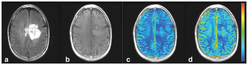
Example pre- and post-STD rCBV images. Shown are the (a) fluid-attenuated inversion recovery images, (b) postcontrast T₁-weighted images, and the (c) pre- and (d) post-STD rCBV maps from one patient (patient 25). Note that while the range of colors in the pre-STD rCBV map is clustered around the center of the color scale, the STD rCBV maps use the full scale of colors.

FIG. 4.

Correlation between pre- and post-STD rCBV data. A near-perfect correlation between STD rCBV and pre-STD rCBV values results for data taken from both the (a) reference ROI (r = 0.9998) and (b) tumor region (r = 0.9999). These data were taken from the same patient whose rCBV maps are shown in Fig. 3.

Figure 5 shows rCBV image maps obtained on three different days for one patient (#24). In the first row (Fig. 5a–c), the rCBV maps are neither normalized nor standardized. In the second row (Fig. 5d–f), the rCBV maps are normalized to a reference normal-appearing white matter ROI manually chosen for each date. Finally, STD rCBV maps are shown in the third row (Fig. 5g–i). Note that the variation across time in the raw and normalized rCBV maps is significantly reduced throughout the normal-appearing brain for the STD rCBV maps. Figure 6 shows the mean values of a reference ROI tracked over time for each subject across all study dates, for raw rCBV maps (Fig. 6a), normalized rCBV maps (Fig. 6b), and STD rCBV maps (Fig. 6c). The coefficient of variation for each of these measurements across time is also shown. Note that standardization results in a significantly reduced variability across study dates, with coefficients of variation ranging from approximately 4–6%, as compared to raw and normalized rCBV maps with much higher coefficients of variation ranging from 9–37%.

FIG. 5.

Longitudinal rCBV maps. The rCBV maps were obtained on three different dates for patient 24. The first row of images (a–c) shows the rCBV maps without standardization or normalization to a reference ROI. The second row of rCBV maps (d–f) shows normalized rCBV maps (g–i), while the third row shows STD rCBV maps.

FIG. 6.

Longitudinal rCBV mean values over time. The rCBV values from the reference ROIs are shown for all three subjects studied longitudinally (24, 25, and 26), for raw rCBV data (a), normalized rCBV data (b), and STD rCBV data (c). Coefficient of variation (CV), a measure of variability introduced by each technique, is given for each of the three subjects.

DISCUSSION

In this study, we have applied the technique of image intensity standardization to rCBV image maps. It is based on transforming the intensity histogram of each rCBV map into a “standard” histogram. This is done in two steps, a training step, which is executed only for once for a given protocol, and a transformation step that is executed for each rCBV map.

With this approach, we have demonstrated that the transformation of rCBV intensities to a standard scale does not corrupt the underlying information. Instead, it shows that the same tissue type has the same rCBV value or “color” for a given color scale. In addition, we have demonstrated that standardization results in greater consistency of rCBV both visually and quantitatively across studies. This result is particularly important if rCBV mapping is to be useful for tracking response to therapies. Given the recent Food and Drug Administration approval of the antivascular therapy bevacizumab (Avastin; Genentech, South San Francisco, CA) for use in patients with primary brain tumors, this development is also particularly timely. Due to its ability to track effects on tumor vascularity, rCBV mapping is quickly becoming a necessary part of evaluating these new therapies (18).

We consistently observed STD rCBV in the range of 5000–7000 arbitrary units for the tumor region, the maximum value of the STD rCBV scale being 50,000. High rCBV values, 90–99.8 percentile, typically come from large vessels such as the sinus, and as such not displaying these highest values negligibly alters the information content presented.

Alternatively, the creation of absolutevalued CBV maps may provide a solution to the variability in the color maps observed with the relative or qualitative rCBV maps (19). However, while in theory this is definitely the case, in practice it is more challenging since the creation of absolute CBV maps require the manual or automatic selection of an arterial input function (20). Manually choosing an arterial input function (AIF) is a very subjective and a time-consuming process. And to date no automatic AIF method has been agreed upon, with many options and theories regarding, for example, using a localized or global AIF. In the end, this too adds error and variability to the maps. For this reason, STD rCBV maps may be the simplest and more robust approach at this time. Future studies are planned to further address this question.

As previously stated (14), there is a tendency to believe that a simple scaling of the minimum to maximum intensity range of a given image to a fixed standard range may resolve the issue of achieving the same values for the same tissues. However, this has been shown not to be the case (11). Alternatively, a method to adjust the contrast and brightness of the MRI images, i.e., a windowing approach, for image display may achieve display uniformity but is not adequate for quantitative image analysis since the intensities still may not have tissue-specific meaning after the windowing transformation. Standardization, described previously (11,12,14) and newly applied to rCBV maps in this paper, offers a simple and reliable way of transforming the images nonlinearly so that there is a significant gain in similarity, as demonstrated for CBV maps. Furthermore, the method is easy to implement and rapid in execution, taking approximately 1 sec to run on a MacBook (Apple, Cupertino, CA) (2.16-GHz Intel Core 2 Duo, 2-GB random-access memory). Thus it can be easily incorporated into the postprocessing algorithms and greatly improve both the visual and quantitative display and analysis of rCBV data.

One potential disadvantage of the standardization technique is the necessity of training the algorithm for each protocol and body part. Through empiric testing we have found that each training file should consist of approximately 15 representative data sets. Slight variations in imaging parameters such as echo time and pulse repetition time and imaging at different field strengths do not affect the transformation. Moreover, as shown in Fig. 2, standardization orders the histogram of rCBV studies enabling STD rCBV values for different tissue types to fall within a range. However, this approach may hide potential global changes in rCBV values, and for this reason it cannot be applied to pathologies or conditions where global changes are expected. Still, as demonstrated in this study, this approach does add tremendous practical value for evaluating changes with local pathologies such as tumor and stroke.

CONCLUSION

From these results, we conclude that the standardization technique translates rCBV values into a standard scale, which accurately represents the original contrast, thus enabling objective visual comparison between patients and dates. From a clinical standpoint, standardization is a simple and elegant solution that should prove very helpful to the radiologists as it makes it unnecessary to subjectively change windowing and contrast on a per-case basis.

References

- 1.Sugahara T, Korogi Y, Shigematsu Y, Liang L, Yoshizumi K, Kitajima M, Takahashi M. Value of dynamic susceptibility contrast magnetic resonance imaging in the evaluation of intracranial tumors. Top Magn Reson Imaging. 1999;10:114–124. doi: 10.1097/00002142-199904000-00004. [DOI] [PubMed] [Google Scholar]
- 2.Aronen HJ, Pardo FS, Kennedy DN, Belliveau JW, Packard SD, Hsu DW, Hochberg FH, Fischman AJ, Rosen BR. High microvascular blood volume is associated with high glucose uptake and tumor angiogenesis in human gliomas. Clin Cancer Res. 2000;6:2189–2200. [PubMed] [Google Scholar]
- 3.Donahue KM, Krouwer HGJ, Rand SD, Pathak AP, Marszalkowski CS, Censky SC, Prost RW. Utility of simultaneously acquired gradient-echo and spin-echo cerebral blood volume and morphology maps in brain tumor patients. Magn Reson Med. 2000;43:845–853. doi: 10.1002/1522-2594(200006)43:6<845::aid-mrm10>3.0.co;2-j. [DOI] [PubMed] [Google Scholar]
- 4.Cha S, Knopp EA, Johnson G, Litt A, Glass J, Gruber ML, Lu S, Zag-zag D. Dynamic contrast-enhanced T2-weighted MRI imaging of recurrent malignant gliomas treated with thalidomide and carboplatin. Am J Neuroradiol. 2000;21:881–890. [PMC free article] [PubMed] [Google Scholar]
- 5.Sugahara T, Jorogi Y, Tomiguchi S, Shigematsu Y, Ikushima I, Kira T, Liang L, Ushio Y, Takahashi M. Posttherapeutic intraaxial brain tumor: the value of perfusion-sensitive contrast-enhanced MR imaging for differentiating tumor recurrence from nonneoplastic contrast-enhancing tissue. Am J Neuroradiol. 2000;21:901–909. [PMC free article] [PubMed] [Google Scholar]
- 6.Law M, Cha S, Knopp EA, Johnson G, Arnett BS, Litt AW. High-grade gliomas and solitary metastases: differentiation by using perfusion and proton spectroscopic MR imaging. Radiology. 2002;222:715–721. doi: 10.1148/radiol.2223010558. [DOI] [PubMed] [Google Scholar]
- 7.Law M, Yang S, Wang H, Babb JS, Johnson G, Cha S, Knopp EA, Zag-zag D. Glioma grading: sensitivity, specificity and predictive values of perfusion MR imaging and proton MR spectroscopic imaging compared to conventional imaging. Am J Neuroradiol. 2003;24:1989–1998. [PMC free article] [PubMed] [Google Scholar]
- 8.Cha S, Johnson G, Wadghiri YZ, Jin O, Babb J, Zagzag D, Turnbull DH. Dynamic, contrast-enhanced perfusion MRI in mouse gliomas: correlation with histopathology. Magn Reson Med. 2003;49:848–855. doi: 10.1002/mrm.10446. [DOI] [PubMed] [Google Scholar]
- 9.Schmainda KM, Rand SD, Joseph AM, Lund R, Ward BD, Pathak AP, Ulmer JL, Baddrudoja MA, Krouwer HGJ. Characterization of a first-pass gradient-echo spin-echo method to predict brain tumor grade and angiogenesis. Am J Neuroradiol. 2004;25:1524–1532. [PMC free article] [PubMed] [Google Scholar]
- 10.Law M, Oh S, Babb JS, Wang E, Inglese M, Zagzag D, Knopp EA, Johnson G. Low-grade gliomas: dynamic susceptibility-weighted contrast-enhanced perfusion MR imaging: prediction of patient clinical response. Radiology. 2006;238:658–667. doi: 10.1148/radiol.2382042180. [DOI] [PubMed] [Google Scholar]
- 11.Nyul LG, Udupa JK, Zhang X. New variants of a method of MRI scale standardization. IEEE Trans Med Imag. 2000;19:143–150. doi: 10.1109/42.836373. [DOI] [PubMed] [Google Scholar]
- 12.Nyul LG, Udupa JK. On standardizing the MR image intensity scale. Magn Reson Med. 1999;42:1072–1081. doi: 10.1002/(sici)1522-2594(199912)42:6<1072::aid-mrm11>3.0.co;2-m. [DOI] [PubMed] [Google Scholar]
- 13.Jensen TR, Schmainda KM. Standardization of relative cerebral blood volume values. Seattle: ISMRM; 2006. p. 441. [Google Scholar]
- 14.Madabhushi A, Udupa JK. New methods of MRI image intensity standardization via generalized scale. Med Phys. 2006;33:3426–3432. doi: 10.1118/1.2335487. [DOI] [PubMed] [Google Scholar]
- 15.Kleihues P, Burger PC, Scheithauer BW. Histological typing of tumours of the central nervous system. New York: Springer-Verlag; 1993. pp. 1–105. [Google Scholar]
- 16.Paulson ES, Schmainda KM. Comparison of dynamic susceptibility-weighted contrast-enhanced mr methods: recommendations for measuring relative cerebral blood volume in brain tumors. Radiology. 2008;249:601–613. doi: 10.1148/radiol.2492071659. [DOI] [PMC free article] [PubMed] [Google Scholar]
- 17.Boxerman J, Schmainda KM, Weisskoff RM. Relative cerebral blood volume maps corrected for contrast agent extravasation significantly correlate with glioma tumor grade whereas uncorrected maps do not. AJR Am J Neuroradiol. 2006;27:859–867. [PMC free article] [PubMed] [Google Scholar]
- 18.Batchelor TT, Sorensen AG, diTomaso E, Zhang W, Duda DG, Cohen KS, Kozak KR, Cahill DP, Chen P-J, Zhu M, Ancukiewicz M, Mrugala MM, Plotkin S, Drappatz J, Louis DN, Ivy P, Scadden DT, Benner T, Loeffler JS, Wen PY, Jain RK. AZD2171, a pan-VEGF receptor tyrosine kinase inhibitor, normalizes tumor vasculature and alleviates edema in glioblastoma patients. Cancer Cell. 2007;11:83–95. doi: 10.1016/j.ccr.2006.11.021. [DOI] [PMC free article] [PubMed] [Google Scholar]
- 19.Sakaie KE, Shin W, Curtis KR, McCarthy RM, Cashen TyA, Carroll TJ. Method for improving the accuracy of quantitative cerebral perfusion imaging. J Magn Reson Imaging. 2005;21:512–519. doi: 10.1002/jmri.20305. [DOI] [PubMed] [Google Scholar]
- 20.Duhamel G, Schlaug G, Alsop DC. Measurement of arterial input functions for dynamic susceptibility contrast magnetic resonance imaging using echoplanar images: comparison of physical simulations with in vivo results. Magn Reson Med. 2006;55:514–523. doi: 10.1002/mrm.20802. [DOI] [PubMed] [Google Scholar]