On the Importance of Well-Calibrated Scores for Identifying Shotgun Proteomics Spectra

Abstract

Identifying the peptide responsible for generating an observed fragmentation spectrum requires scoring a collection of candidate peptides and then identifying the peptide that achieves the highest score. However, analysis of a large collection of such spectra requires that the score assigned to one spectrum be well-calibrated with respect to the scores assigned to other spectra. In this work, we define the notion of calibration in the context of shotgun proteomics spectrum identification, and we introduce a simple, albeit computationally intensive, technique to calibrate an arbitrary score function. We demonstrate that this calibration procedure yields an increased number of identified spectra at a fixed false discovery rate (FDR) threshold. We also show that proper calibration of scores has a surprising effect on a previously described FDR estimation procedure, making the procedure less conservative. Finally, we provide empirical results suggesting that even partial calibration, which is much less computationally demanding, can yield significant increases in spectrum identification. Overall, we argue that accurate shotgun proteomics analysis requires careful attention to score calibration.

1. Introduction

The core of any high-throughput shotgun proteomics analysis pipeline is a procedure for assigning peptide sequences to observed fragmentation spectra. Typically, this assignment is done by treating each spectrum as an independent observation and then iteratively scoring the spectrum against a given database of peptides, considering only those candidate peptides whose masses lie within a specified tolerance of the precursor mass associated with the observed spectrum. The top-scoring candidate peptide is then assigned to the spectrum, resulting in a peptide–spectrum match (PSM). Sometimes the resulting PSM is correct, the peptide assigned to the spectrum was present in the mass spectrometer when the spectrum was generated, and sometimes the PSM is incorrect. Therefore, after a PSM is created for each observed spectrum, the PSMs are sorted by score, and a threshold is selected such that the PSMs scoring above the threshold (accepted PSMs) have a specified false discovery rate, defined as the estimated percentage of accepted PSMs that are incorrect.

An important but under-appreciated aspect of this spectrum identification protocol is that the score function used to compare a peptide to a spectrum is being asked to do two jobs at once. First, the score function must identify which candidate peptide best matches a particular observed spectrum. Second, the same score function must rank the full set of PSMs in such a way that correct PSMs outrank incorrect ones.

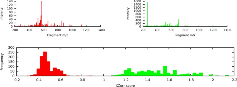
What might not be immediately obvious is that a given score function might be very good at the first of these two tasks and very bad at the second. To see that this is the case, consider a hypothetical score function that depends strongly upon the total number of peaks in the observed spectrum. Consequently, candidate peptides scored with respect to spectrum σ_i receive scores in the range, say, 0 to 1, whereas candidate peptides scored with respect to spectrum σ_j receive scores in the range 1 to 2. In this scenario, even if the score function identifies the correct candidate peptide for σ_i, the resulting PSM can never out-rank the PSM for σ_j. This is undesirable if, in fact, the score function incorrectly identifies σ_j. An example of this phenomenon is shown in Figure 1, where the SEQUEST score function XCorr¹ assigned scores to 1000 randomly drawn shuffled candidate peptides (decoys) for two different spectra. The spectrum σ₁₄ yields scores in the range 0.29–0.89, whereas the spectrum σ₇₁₆ yields scores in the range 1.0–2.2. Because the two corresponding histograms do not overlap, if we use XCorr, then all of the 1000 peptide matches to σ₇₁₆ are considered to be better than all of the 1000 peptide matches to σ₁₄. Intuitively, this is unreasonable: because these PSMs were found by scoring decoy peptides, we expect the two histograms to look quite similar.

Figure 1.

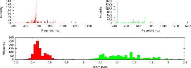
Calibrated vs raw PSM scores. Two spectra, σ₁₄ (red) and σ₇₁₆ (green), and the corresponding histograms of XCorr scores generated by searching each spectrum against 1000 randomly drawn decoys. The spectra are taken from the yeast data set.

The underlying issue here is that the XCorr score is not well-calibrated. We say that a PSM score function is well-calibrated with respect to spectra if a score of x assigned to spectrum σ_i has the same meaning or significance as a score of x assigned to spectrum σ_j. Note that the notion of calibration can be defined relative to any arbitrary partition of the PSMs, for example, based on peptide length, precursor mass, total ion current, precursor charge, etc. In practice, many PSM score functions are not well-calibrated with respect to spectra. As in Figure 1, they tend to assign systematically different scores to different spectra. Therefore, we cannot use these scores to directly compare the quality of PSMs involving two different spectra.

Our primary goal in this article is to call attention to the importance of score calibration in the context of shotgun proteomics analysis. It is important to recognize that simply creating a score with a well-defined semantics, based on a probabilistic model,²⁻⁴ on empirical p-values derived from a large collection of decoy PSMs,⁵ or on p-values created by fitting scores from many spectra to a parametric distribution,⁶ does not address calibration as we have defined it because the above methods do not take into account the statistics specific to each spectrum. On the other hand, transforming scores separately for each spectrum can indeed lead to better calibration. This can be accomplished by fitting scores to a Poisson,⁷ exponential,^8,9 or Gumbel distribution.^10,11 Alternatively, dynamic programming can be used to enumerate the entire distribution of a particular score function over all possible peptide sequences, yielding exact p-values that condition on the spectrum,¹²⁻¹⁴ provided that the score function can be represented as a sum of independent terms. Alves et al.¹⁵ describe a generic methodology for calibrating PSM scores that uses a collection of reference spectra, searched against a decoy database, to fit a calibration function for any given scoring scheme. However, in this case, the calibration is intended to address the variability across different search tools (for a given spectrum) rather than the variability across spectra. Finally, another class of methods addresses per-spectrum calibration by employing a machine learning postprocessor, such as linear discriminant analysis¹⁶ or support vector machines.¹⁷⁻¹⁹ This type of postprocessor can account for spectrum-specific effects when appropriate spectrum features are provided as input to the algorithm.

The large diversity in approaches to assigning significance to a PSM that is evident in the above review underlines the difficulty in score calibration. It stands to reason that every one of the proposed methods is well-suited for some tasks, but there does not seem to be any one method to rule them all. Indeed, we give evidence below that two of the more theoretically supported methods, one that relies on the assumption that the score of the optimal PSM follows a Gumbel distribution^10,11 and another that uses exact p-values,¹² do not always achieve optimal calibration. In light of this observation and given that our primary goal here is to study the effects of calibration, rather than the optimal practical way to achieve it, we propose a different approach here, one that asymptotically guarantees calibration while requiring only minimal theoretical assumptions.

We begin by introducing a straightforward but computationally expensive method for empirically calibrating an arbitrary PSM score function. Note that, due to its computational expense, we do not propose that this calibration procedure provides the best practical tool for the job; rather, we use the procedure to study the calibration properties of several existing approaches. In particular, we demonstrate on several different combinations of data sets and scoring functions the significant positive impact that calibration has on our ability to identify spectra at a specified false discovery rate threshold, using a standard decoy-based estimation procedure called target–decoy competition (TDC).²⁰ We then investigate an alternative method for estimating the false discovery rate, previously proposed by one of us,²¹ and show that calibrating the PSM scores has a surprising effect on this procedure, making it more liberal than TDC. Finally, we investigate the trade-off between calibration and computational expense, showing that even partial calibration can lead to significant improvements in performance.

2. Materials and Methods

2.1. Data

Analysis was performed using three previously described sets of spectra (Table 1). All three data sets and their associated protein databases are available at http://noble.gs.washington.edu/proj/calibration.

Table 1. Properties of the Three Data Sets.

data set	yeast	worm	Plasmodium
precursor resolution	low	high	high
fragment resolution	low	low	high
+1 spectra	737	1423	—
+2 spectra	34 499	7891	1311
+3 spectra	34 469	4646	8441
+4 spectra		1683	2372
+1 PSMs	737	241	—
+2 PSMs	34 499	4494	790
+3 PSMs	34 467	3173	8382
+4 PSMs		1288	2362
enzyme	trypsin	trypsin	lys-c
peptides in database	165 930	462 523	223 602
precursor m/z tolerance	±3 Th	±10 ppm	±50 ppm
fragment m/z bin width	1.0005079	1.0005079	0.10005079
average candidates/spectrum	955.7	22.0	48.7

The yeast data set was collected from Saccharomyces cerevisiae (strain S288C) whole-cell lysate.¹⁹ The cells were cultured in YPD media, grown to mid log phase at 30 °C, lysed, and solubilized in 0.1% RapiGest. Digestion was performed with a modified trypsin (Promega), and the sample was subsequently microcentrifuged at 14 000 rpm to remove any insoluble material. Microcapillary liquid chromatography tandem mass spectrometry was performed using 60 cm of fused silica capillary tubing (75 μm i.d.; Polymicro Technologies), placed in-line with an Agilent 1100 HPLC system and an LTQ ion trap mass spectrometer. MS/MS spectra were acquired using data-dependent acquisition with a single MS survey scan triggering five MS/MS scans. Precursor ions were isolated using a 2 m/z isolation window. The charge state of each spectrum was estimated by a simple heuristic that distinguishes between singly charged and multiply charged peptides using the fraction of the measured signal above and below the precuror m/z.²⁶ No attempt to distinguish between 2+ or 3+ spectra was made other than limiting the database search to peptides with a calculated M + H mass of 700 to 4000 Da. Thus, of the 35 236 spectra, 737 were searched at 1+ charge state, 30 were searched at 2+ charge state, and the remaining (34 469) were searched at both 2+ and 3+ charge states.

The worm data set is derived from a Caenorhabditis elegans digest.²⁷C. elegans were grown to various developmental stages on peptone plates containing Escherichia coli. After removal from the plate, bacterial contamination was removed by sucrose floating. The lysate was sonicated and digested with trypsin. The digest (4 μg) was loaded from the autosampler onto a fused-silica capillary column (75 μm i.d.) packed with 40 cm of Jupiter C12 material (Phenomenex) mounted in an in-house constructed microspray source and placed in line with a Waters NanoAcquity HPLC and autosampler. The column length and HPLC were chosen specifically to provide highly reproducible chromatography between technical replicates, as previously described.²⁷ Tandem mass spectra were acquired using data-dependent acquisition with dynamic exclusion turned on. Each high-resolution precursor mass spectrum was acquired at 60 000 resolution (at m/z 400) in the Orbitrap mass analyzer in parallel with five low-resolution MS/MS spectra acquired in the LTQ. Bullseye²⁸ was then used to assign charges and high-resolution precursor masses to each observed spectrum on the basis of persistent peptide isotope distributions. Because a single precursor m/z range may contain multiple such distributions, Bullseye frequently assigns more than one distinct precursor charge and mass to a given fragmentation spectrum. The final data set consists of 7557 fragmentation spectra, with an average of 2.10 distinct precursors per spectrum: 1423 +1, 7891 +2, 4646 +3, 1683 +4, and 228 +5. The +5 spectra were discarded from the analysis.

The Plasmodium data set is derived from a recent study of the erythrocytic cycle of the malaria parasite Plasmodium falciparum.²⁹P. falciparum 3D7 parasites were synchronized and harvested in duplicate at three different time points during the erythrocytic cycle: ring (16 ± 4 h postinvasion), trophozoite (26 ± 4 h postinvasion), and schizont (36 ± 4 h postinvasion). Parasites were lysed, and duplicate samples were reduced, alkylated, digested with Lys-C, and then labeled with one of six TMT isobaric labeling reagents. The resulting peptides were mixed together, fractionated via strong cation exchange into 20 fractions, desalted, and then analyzed via LC–MS/MS on an LTQ-Velos-Orbitrap mass spectrometer. All MS/MS spectra were acquired at high resolution in the Orbitrap. We focused on one of these fractions (number 10), consisting of 12 594 spectra, and we discarded 470 spectra with charge state > +4, leaving 12 124 spectra.

2.2. Assigning Peptides to Spectra

Searches were carried out using two different search engines: the Tide search engine,²² as implemented in Crux v2.0,³⁰ and MS-GF+.¹²

The yeast spectra were searched against a fully tryptic database of yeast proteins. The trypsin cleavage rule did not include suppression of cleavages via proline.³¹ The precursor m/z window was ±3.0 Th. No missed cleavages were allowed, and monoisotopic masses were employed for both precursor and fragment masses. A static modification of C + 57.02146 was included to account for carbamidomethylation of cysteine. For Tide, the mz-bin-width parameter was left at its default value of 1.0005079. For MS-GF+, the -inst parameter was set to 0, and no isotope errors were allowed.

The worm spectra were searched against a fully tryptic database of C. elegans proteins plus common contaminants. Searches were performed using the same parameters as for the yeast data set, except that candidate peptides were selected using a precursor tolerance of 10 ppm. For MS-GF+, the -inst parameter was set to 1, and no isotope errors were allowed. Note that, due to the Bullseye processing of the worm spectra, a single spectrum may have been assigned multiple high-resolution precursor windows with the same charge state. In such cases, we identified the maximum scoring PSM per charge state. Eliminating spectra with no Bullseye-assigned precursor window or no candidate peptides within the assigned precursor range yielded a total of 9312 worm PSMs.

The Plasmodium spectra were searched against a database of Plasmodium peptides, digested using Lys-C. In addition to C + 57.02146, static modifications of +229.16293 were applied to lysine and to the peptide N-termini to account for TMT labeling. All searches were performed using a 50 ppm precursor range. For Tide, the mz-bin-width parameter was set to 0.10005079. For MS-GF+, the -inst parameter was set to 1, and no isotope errors were allowed. For some spectra, no candidate peptides occur within the specified precursor tolerance window; hence, the number of PSMs (11 625) is smaller than the total number of spectra (12 594).

As noted below, a subset of the results, Table 2 and Figures 9 and 10, were obtained using the XCorr score computed by the search-for-matches search engine in Crux v1.39.²³

Table 2. Variability in PSM Discoveries Reported by Different Applications of TDC Using Calibrated and Raw XCorr Scores.

		% only in one T-TDC raw score			% only in one T-TDC calibrated score
set	FDR	0.01	0.05	0.10	0.01	0.05	0.10
yeast	0.05 quantile	0.1	0.5	1.1	0.0	0.1	0.3
	median	1.0	0.9	1.6	0.6	0.6	0.8
	0.95 quantile	3.1	2.1	2.8	2.4	1.7	2.0
worm	0.05 quantile	0.1	0.6	1.5	0.0	0.2	0.5
	median	1.5	1.5	2.5	1.1	0.8	1.2
	0.95 quantile	4.7	3.5	4.6	3.9	2.5	3.0
Plasmodium	0.05 quantile	0.0	0.6	1.4	0.0	0.1	0.2
	median	1.1	1.3	2.2	0.6	0.5	0.7
	0.95 quantile	6.0	3.3	3.9	2.6	1.6	2.3

Figure 9.

Decoy-estimated p-values: calibrated versus raw scores. The target PSM p-values were estimated from XCorr scores in three different ways: (i) p-values were estimated using the same 10K decoys per spectrum that we use to define our calibrated scores or (ii, iii) a single-decoy set was arbitrarily chosen and used to estimate the target PSM p-value according to Käll’s procedure, but once using the raw scores for both decoy and target PSMs and another time using the calibrated scores for both. (A) Scatter plot of raw score p-values (yeast, charge 2 set) computed using Käll’s procedure (a single-decoy set, y axis) and using spectrum-specific distributions generated from 10K decoys (x axis). (B) Similar to panel A, but computed using calibrated rather than raw scores. (C) The figure plots, as a function of p-value threshold, the fraction of target PSMs with p-values less than or equal to the threshold. For any nominal p-value t ≤ 0.95, we find fewer target PSMs whose raw score estimated p-value is ≤ t (blue) than when the same p-value is estimated using the calibrated scores with either the single-decoy or per-spectrum method (magenta and green, essentially in perfect agreement).

Figure 10.

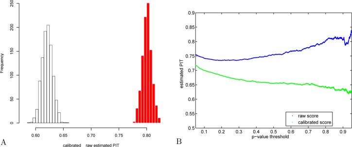
Estimating Käll’s percentage of incorrect targets: calibrated versus raw scores. (A) The value of π₀ in the yeast charge 2 optimal target PSM set was estimated separately using each of 1000 decoy sets. The red histogram corresponds to raw XCorr scores, and the white, to calibrated scores. (B) Using the first decoy set, π₀ was estimated using a fixed p-value threshold (again, yeast charge 2 set). The increasing trend that troubled Käll et al.²¹ (Figure 6B in their paper) is visible in blue here when using the raw score, but it disappears when the estimate is based on calibrated score (green).

2.3. Decoy Generation

Decoy databases were generated by independently shuffling the nonterminal amino acids of each distinct target peptide. For each database, the decoy creation procedure was repeated 11 000 times, creating a 10K decoy set (used for calibration as explained next) and an independent 1K decoy set (used for evaluating the performance of the search methods).

2.4. Calibrating the Scores

The raw score we use in our database searches is SEQUEST’s XCorr.¹ For each spectrum σ in each of our charge sets, we use Crux²³ to find the XCorr score of the best match of σ against the peptide database DB:

Our calibration of the raw score is spectrum-specific: we replace s = S(σ, db) by an estimate of the p-value of s

where db is the target database and DB is a decoy database that is randomly generated as described above.

The p-value is estimated using a straightforward Monte Carlo scheme: each spectrum σ is searched against each decoy database dc in the 10K decoy set, and the optimal (raw score) PSM for that database z = S(σ,dc) is noted (we loosely refer to these as the decoy PSMs). We next use this null sample of N = 10 000 decoy PSM scores {z_i}_i=1^N to construct a spectrum-specific empirical null distribution. This distribution is then used to assign the spectrum-specific p-value of an observed raw score s = S(σ, db), which is essentially the rank of s in the combined list of s and {z_i}. Technically, the calibrated score is the negative of the empirically estimated p-value.

Note that we can use this procedure to calibrate optimal PSMs generated by searching either the target database db or any of the decoy databases dc in the 1K decoy set. We stress that the 1K set is disjoint from the 10K decoy set that is used to calibrate the scores.

For the 1K decoy calibration, we used the first 1000 decoys of the 10K decoy set to estimate the empirical distribution of the spectrum-specific optimal PSM.

2.5. Estimating FDR Using Target–Decoy Competition

In target–decoy competition, the number of false or incorrect PSMs is estimated by searching a decoy database. Specifically, a decoy database of the same size as the target database is drawn according to the null model of choice (shuffling in our case, Section 2.3), and each spectrum is searched against the concatenated database, retaining the single best-scoring PSM for each spectrum. The concatenation of the database creates a target–decoy competition, where any optimal target PSM that scores less than the corresponding optimal decoy PSM is eliminated from consideration.

Here, we use a target-only version of the TDC procedure, where the list of reported discoveries consists only of those PSMs that score higher than the threshold and that are matched with a target peptide from the concatenated database. The number of false discoveries in this filtered discovery list is estimated by the number of PSMs whose score exceeds the threshold and that are matched to a decoy peptide in the concatenated database. The FDR at level t is then estimated by the ratio of the number of decoy to target PSMs that exceed the level t.

2.6. Estimating FDR Using the Käll Procedure

Executing two separate searches, one against the target database and one against the randomly drawn decoy database, the Käll procedure uses the set of optimal decoy PSM scores to estimate the p-values of optimal target PSMs. Applying the standard FDR analysis of Storey³² to these target PSM p-values, the Käll procedure estimates π₀, the proportion of incorrect target hits.

The list of discoveries at threshold t includes all target PSMs that score above t. Unlike TDC, no target–decoy competition is done; however, like TDC, decoys are filtered out of the reported list of discoveries. The number of false discoveries in that list is estimated by the product of π₀ and the number of decoy PSMs that score above t. The estimated FDR at level t is then the ratio of these two numbers.

2.7. Number of Discoveries at a Given FDR

Note that for both TDC and the Käll procedure, the estimated FDR is not necessarily a monotone function of the score threshold t. Hence, when determining a score cutoff to achieve a desired FDR threshold α, the procedure is to select the most permissive (lowest) cutoff score t for which the FDR is still ≤α. For computational efficiency, we computed this number for only 120 selected values of α: from 0.001 to 0.01 in increments of 0.001, from 0.012 to 0.05 in increments of 0.002, and from 0.055 to 0.5 in increments of 0.005.

2.8. Evaluating the Differences in Discovery Lists

The differences in the discovery lists between methods A and B were evaluated at a given FDR level α ∈ {0.01,0.05,0.1} as follows. First, we identified the largest discovery list reported by each method for which the FDR was still ≤α. Then, the two lists were compared to see which PSMs appear only in A and not in B and vice versa. Finally, the number of PSMs present only in A’s list was expressed as a percentage of the total number of PSMs in this list (and vice versa).

3. Results

3.1. A Procedure for Producing Calibrated Scores

One common way to calibrate scores is to assign them a p-value. Suppose that the top-scoring PSM produced by scanning a spectrum σ against a peptide database has score s. The p-value of s is defined as the probability of observing an optimal match with a score ≥ s, assuming that the spectrum σ is scanned against a randomly drawn database. Because this procedure assigns to each PSM a universal measure of surprise, we can use the resulting p-values to directly compare PSMs regardless of whether they share the same spectrum: the smallest p-value indicates the largest level of surprise and should therefore coincide with the most promising match.

Of course, this definition of p-value depends on the notion of a randomly drawn database, known more generally as the null model. In the best case, the null model can be characterized analytically, and the corresponding p-value can be calculated exactly. This is the approach taken by most familiar statistical tests, such as a t-test or χ²-test. If, however, the null model is too unwieldy to allow an exact computation of the p-value, then one can always rely on a Monte Carlo estimation if one has sufficient computational resources.

In our case, we propose a straightforward Monte Carlo scheme for estimating PSM p-values (Section 2.4). The procedure involves creating multiple databases according to a specific null model, in which nonterminal amino acids in each peptide are shuffled uniformly at random. We refer to these shuffled databases as decoy databases and to the original database as the target database. We then scan each decoy database for matches against σ, and we record the best PSM for each random database. Using the resulting scores, we generate an empirical null distribution for each spectrum, which is then used to assign the p-value of the best match of σ against the target database. This p-value is our calibrated score.

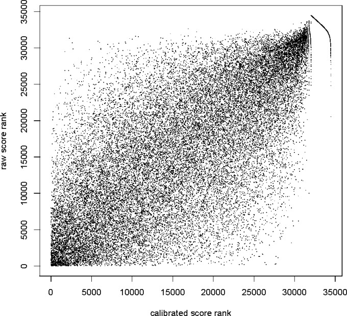
To understand the impact of calibration in practice, consider again the two tasks mentioned above: identifying which candidate peptide best matches a particular observed spectrum, and ranking the full set of PSMs in such a way that correct PSMs outrank incorrect ones. Because calibration is carried out separately for each spectrum, it should be clear that calibration will not affect the first task: the best PSM for a given spectrum is the same regardless of whether the score is calibrated. However, the changes in the ranking of PSMs involving different spectra can be substantial (Figure 2).

Figure 2.

Calibration changes the ranking of PSMs. Scatter plot of calibrated versus raw XCorr score rank of each optimal PSM from 34 469 +3 spectra from the yeast data set. The tail at the right end of the graph consist of 2438 PSMs with the same minimal calibrated score (maximal p-value), so their calibrated rank is somewhat arbitrarily determined within that set of poorly scored PSMs. Similar figures (not shown) were obtained for all other data sets that we examined.

3.2. The Impact of Calibration on Statistical Power Assessed Using Target–Decoy Competition

Given calibration’s substantial impact on the ranking of PSMs, we expect calibration to have a corresponding impact on the number of spectra successfully identified as a function of FDR threshold. Ideally, we would like the calibration procedure to boost our statistical power, which is defined in this setting as the probability of correctly identifying the correct PSM. From a practical perspective, improving statistical power corresponds to increasing the number of spectra identified at a fixed FDR threshold.

To assess the effect of calibration on statistical power, we employed a previously described, decoy-based method for estimating false discovery rate, called target–decoy competition (TDC).²⁰ Briefly, the method consists of searching a given set of spectra against a database containing an equal number of target and decoy peptides, retaining the single best-scoring PSM for each spectrum. As a result of this selection, any optimal target PSM that scores less than the corresponding optimal decoy PSM is eliminated from consideration. Subsequently, at a given score threshold, the number of accepted decoy PSMs provides an estimate of the number of accepted incorrect target PSMs. Note that, in this work, we use a variant of the originally proposed TDC protocol, in which we estimate the FDR with respect to the list of target PSMs rather than with respect to the combined list of target and decoy PSMs (Materials and Methods, Section 2.5).

It is intuitively clear that our simple calibration procedure does not depend on the particular score function. However, the magnitude of the improvement achieved via calibration obviously varies according to how well or ill calibrated the score function is. We therefore looked at three different score functions: the SEQUEST XCorr score, as implemented in the Tide search tool,²² the MS-GF+ raw score, and the MS-GF+ E-value.¹² Note that MS-GF+ E-value is designed as a calibrated score function, so, in principle, our calibration procedure should not be able to improve it.

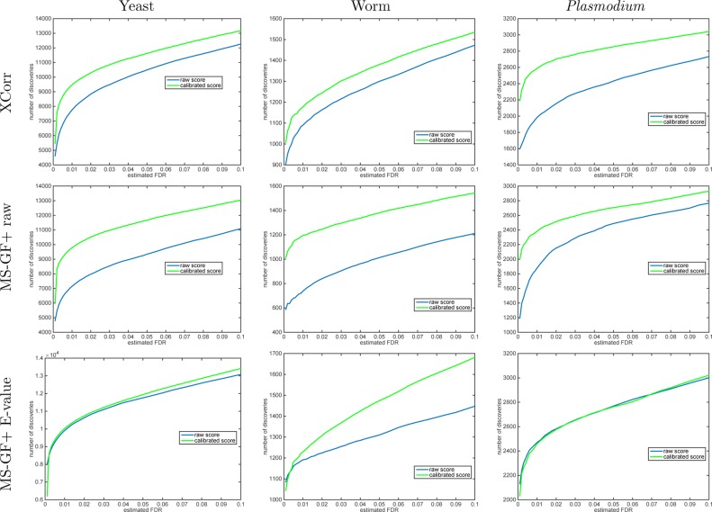
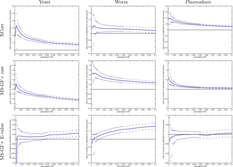
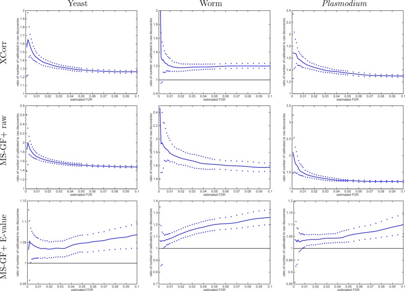
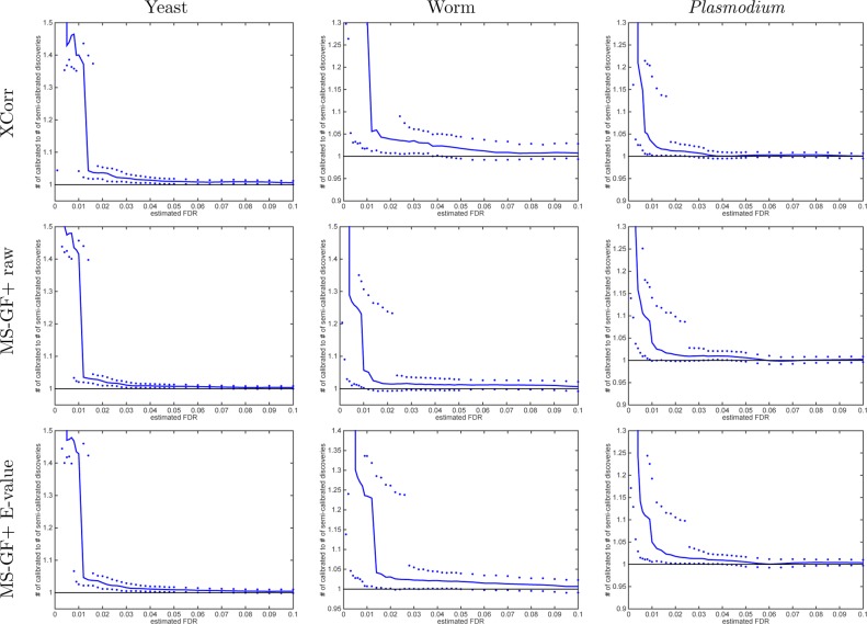
Using TDC, we find that calibrating the scores yields more discoveries across the entire practical range of FDR values for both XCorr and MS-GF+ raw scores and across all three data sets that we examined (Figures 3 and 4). At FDR 1% and using Xcorr, we observe an increase in the number of discoveries of 22, 8.0, and 31% for the yeast, worm, and Plasmodium data sets, respectively. Using the MS-GF+ raw score, the corresponding improvements at the same 1% FDR level are 37, 61, and 27%. Presumably, MS-GF+’s raw score is even less calibrated than XCorr. Note that these are median improvements across 1000 raw-vs-calibrated applications of TDC to that many independently drawn decoy databases. This improvement in statistical power occurs because when we sort PSMs according to their calibrated score, higher quality PSMs are moved higher up the list. In the context of target–decoy competition, these higher quality PSMs are less likely to be surpassed by corresponding decoy matches. In the end, the increased number of discoveries provides strong motivation to perform score calibration as part of any mass spectrometry identification procedure.

Figure 3.

Calibrating a noncalibrated score, on average, yields more discoveries (TDC). Each panel plots the median number of discoveries as a function of FDR threshold using TDC applied to the raw and calibrated scores (the median is with respect to 1000 applications, each using a single independently drawn decoy set). Calibration substantially increases the number of TDC discoveries when using the noncalibrated MS-GF+ and Xcorr scores. MS-GF+ E-value is designed as a calibrated score; hence, calibration adds little to the yeast and Plasmodium data sets. Surprisingly, though, calibration makes a substantial impact even on the E-value in the worm data set.

Figure 4.

Calibrating a noncalibrated score mostly yields more discoveries (TDC). Each panel plots, as a function of estimated FDR, the ratio of the number of TDC discoveries at FDR ≤ 0.1 when using the calibrated score (numerator) versus the number of discoveries at the same FDR when using the raw score (denominator). The solid line represents the median ratio (with respect to 1000 ratios, each comparing the raw vs calibrated TDC discoveries using a single independently drawn decoy set), whereas the 0.95 and 0.05 quantiles of the ratios are represented as dots. For small FDR values, the calibrated score yields considerably more discoveries than the uncalibrated score (MS-GF+ and Xcorr).

An additional benefit that calibration provides is a reduction in the variability in the list of identified spectra. This variability arises because of the random nature of the decoys in TDC: the set of target PSMs that win the target–decoy competition differs each time the procedure is run. Note that the use of reversed, rather than shuffled, decoy peptides simply hides this problem by arbitrarily fixing the decoys and the corresponding filtered peptides. To quantify the amount of decoy-induced variation in the list of discoveries, we randomly drew 2000 nonidentical pairs of decoys from our list of 1000 independent decoy sets and recorded, for a few selected levels of FDR, the number of discoveries that are found in one application of TDC and not the other (Materials and Methods, Section 2.8). The results (Table 2) show that the decoy-induced median variation in the composition of the discovery list is smaller when using the calibrated score than when using the raw score. Note that these results, as well as those in Figures 9 and 10, were obtained using the XCorr score as implemented in the Crux tool search-for-matches.²³

The MS-GF+ E-value score is designed to be calibrated; thus, it is not surprising that at 1% FDR level there is little difference between using the E-value score and its 10K-calibrated version: 1.2 and 3.3% more calibrated TDC discoveries in the yeast and worm data sets, respectively, and 0.5% fewer discoveries in the Plasmodium data set. Similarly, at 5% FDR level, the calibrated version of the MS-GF+ E-value identifies 1.5% more discoveries in the yeast data set and 0.2% fewer discoveries in the Plasmodium data set. It is, however, surprising that at the same 5% FDR level the calibrated version yields 12% more discoveries in the worm data and that number increases to 16% at 10% FDR level. We suspect that some of the assumptions that go into computing the MS-GF+ E-value are violated for the worm data set, but these do not affect our robust albeit costly calibration procedure.

3.3. Calibration’s Effect on the Method of Käll et al

To further investigate the effect of calibration on the statistical analysis of PSMs, we considered an alternative method for estimating the FDR, proposed by Käll et al.²¹ The method differs from the TDC method in two ways (Materials and Methods, Section 2.6). First, the Käll method estimates the FDR by using the empirical distribution function of all of the optimal decoy PSMs, rather than just those optimal decoy PSMs that win the target–decoy competition. Similarly, the list of accepted target PSMs from the Käll method includes all of the optimal target PSMs that score above a certain threshold, regardless of whether they win the target–decoy competition. Second, the Käll method requires estimation of a parameter π₀, representing the percentage of the optimal target PSMs that are incorrect. The final FDR estimate includes π₀ as a multiplicative factor.

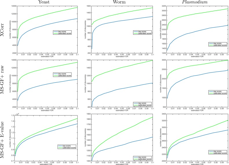
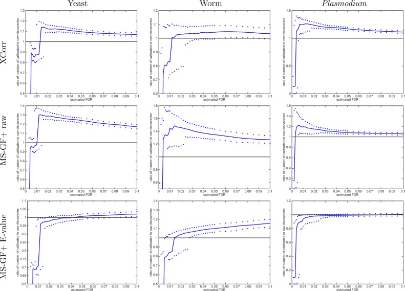
Similar to the TDC procedure, using Käll’s procedure with calibrated scores yields a significant boost in the number of discoveries across the entire range of practical FDR thresholds (Figures 5 and 6). For example, at FDR 1%, Käll’s method suggests that when using XCorr calibration increases the number of discoveries by 43, 20, and 53% for the yeast, worm, and Plasmodium data sets (again, these are median improvements using 1000 independently drawn decoy sets). Notably, this increase in the number of discoveries is substantially larger than we observed previously for TDC using XCorr, which yielded corresponding percentages of 22, 8.0, and 31%. The corresponding increases at 1% FDR when using MS-GF+’s raw score are 70, 79, and 49% for the 10K-calibrated Käll’s method over using the raw score (compared with 37, 61, and 27% increases when using TDC).

Figure 5.

A calibrated score, on average, yields more discoveries (Käll). Each panel plots the median number of discoveries as a function of FDR threshold using the Käll method applied to the raw and calibrated scores (the median is with respect 1000 applications, each using a single independently drawn decoy set). For small FDR values, the calibrated score yields considerably more discoveries than the uncalibrated score. Note that even for MS-GF+ E-value our calibration procedure typically increases the number of Käll discoveries.

Figure 6.

A calibrated score mostly yields more discoveries (Käll). Each panel plots, as a function of estimated FDR, the ratio of the number of Käll method discoveries at FDR ≤ 0.1 when using the calibrated score (numerator) versus the number of discoveries at the same FDR when using the raw score (denominator). The solid line represents the median ratio with respect to 1000 independently drawn decoy sets, whereas the 0.95 and 0.05 quantiles of the ratios are represented as dots.

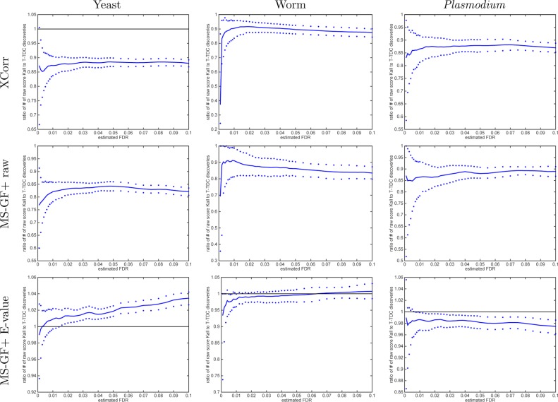
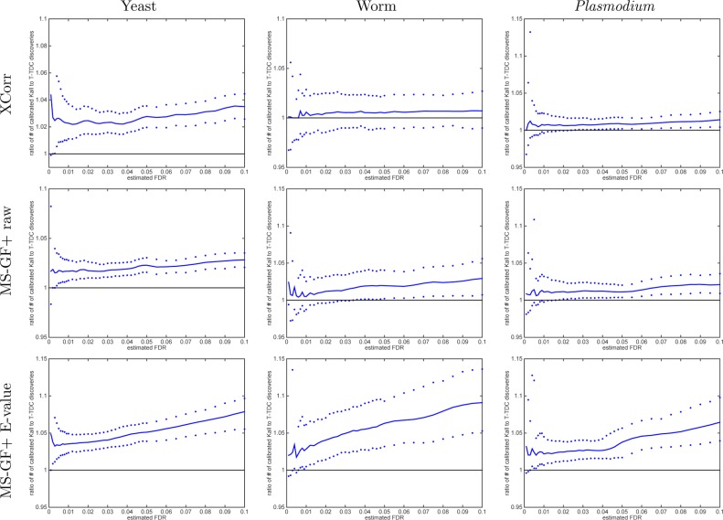
To better understand this difference, we directly compared the number of discoveries produced by the two methods as a function of FDR threshold. Surprisingly, this comparison yields opposite results depending upon whether we use calibrated or noncalibrated scores. Using noncalibrated scores (Xcorr, MS-GF+ raw score), the TDC procedure systematically yields more discoveries than the Käll procedure (Figure 7), whereas the behavior is reversed when we use calibrated scores (Figure 8).

Figure 7.

With noncalibrated scores, Käll’s method is more conservative than TDC. The ratio of the number of Käll discoveries to TDC discoveries at FDR ≤ 0.1 when using the raw score. The median ratio (with respect to 1000 independently drawn decoys) in solid line is flanked by the 0.95 and 0.05 quantiles of the ratios. Results are for raw scores, but keep in mind that MS-GF+ E-value is partially calibrated even in its raw form, so the ratio of Käll to TDC discoveries fluctuates above and below 1.

Figure 8.

With calibrated scores, Käll’s method gives more discoveries than TDC. The ratio of the number of Käll discoveries to TDC discoveries at FDR ≤ 0.1 when using the calibrated score. The median ratio (with respect to 1000 independently drawn decoys) in solid line is flanked by the 0.95 and 0.05 quantiles of the ratios. After calibrating, all three scores typically yield more Käll than TDC discoveries at any given FDR.

We claim that this reversal in behavior arises because the Käll procedure implicitly assumes a calibrated score. Recall that the Käll procedure estimates the p-value of each PSM by using the empirical score distribution from a single set of decoy PSMs. If the score is not calibrated, then the resulting p-values can differ substantially from the p-value that we estimate using 10 000 sets of decoys. To illustrate this phenomenon, we estimated the p-value of each target PSM raw score (yeast, charge 2 set) in two different ways: by constructing a single distribution of optimal PSM scores from a single decoy set (single-decoy p-values) and by constructing spectrum-specific distributions using 10 000 decoy sets (per-spectrum p-values). The two resulting sets of p-values are positively correlated (Pearson correlation of 0.825) but exhibit substantial differences (Figure 9A). Because the per-spectrum p-value accounts for spectrum-to-spectrum variability in scores, we conclude that the single-decoy p-values estimated by the Käll procedure method from raw scores are inaccurate. In contrast, when we switch to calibrated scores and repeat this comparison, the single-decoy and per-spectrum p-values are in almost perfect agreement (Figure 9B, Pearson correlation of 1.000). Thus, the Käll procedure yields accurate p-values only when the given scores are well-calibrated.

In our example, the inaccuracies in estimating the p-values based on raw scores accumulate to yield an overall conservative bias in the estimated single-decoy p-values (Figure 9C, blue curve). In contrast, the analogous curves generated when using the calibrated scores with per-decoy p-values (green) or per-spectrum p-values (magenta) perfectly overlap.

This conservative bias has two undesired consequences. First, higher (more conservative) p-values means fewer discoveries (Figure 5). Second, it also means that the percentage of incorrect targets, π₀, is incorrectly estimated because the estimation relies on correctly estimated p-values. To demonstrate the effect of calibration on estimating π₀, using each of 1000 randomly drawn decoy sets, we estimated π₀ in the list of target PSMs generated by scanning the yeast charge 2 spectra set against the target database. This was done twice: once when both target and decoy PSM were evaluated using the raw scores and once using the calibrated scores for both. We estimated π₀ using the smoother option in the R function qvalue. Clearly, using the calibrated score yields a significantly lower (less conservative) estimate of π₀ (Figure 10A). This result is problematic because the value of π₀ should not depend on which score we use.

Interestingly, Käll et al.²¹ reported a problem they observed in estimating π₀ (Figure 6B in ref (21)): “The increasing trend in the plot is evidence of a conservative null model. Apparently, there is an enrichment of target PSMs with very low scores, which likely correspond to poor quality spectra. A significant avenue for future research is finding a better null model that does not yield this type of artifact.” In our experiments, when we estimated π₀ using the raw scores, we observed the same problem (Figure 10B, blue curve). However, when the same procedure is applied to the calibrated scores, the problematic increasing trend is all but gone (green curve).

3.4. How Many Decoys Do We Need for Calibration?

To calibrate our scores, here we paid a hefty price: multiplying the search time by a factor of 10 000. While for a small set of spectra and a reasonably sized peptide database this approach might be feasible, analysis of larger data sets would require considerable computing resources. It is therefore natural to ask whether we can still enjoy some of the benefits of calibration if we use only a semicalibrated score, say by calibrating using only 1000 decoys (1K calibration). Note that, as with the 10K decoy calibration, these 1K decoys are independent of the 1000 decoy sets used for the target decoy analysis. In fact, here we simply use the first 1000 of the decoy sets used for the full 10K calibration.

Our experiments suggest that semicalibrated scores are useful, as long as we do not seek to set the FDR threshold too low. In particular, when we use an FDR threshold (estimated via TDC) in the range of 2–10%, the semicalibrated scores yield improved performance relative to noncalibrated scores (Xcorr and MS-GF+ raw score) across all three data sets that we examined (Figure 11). Especially for thresholds of 5 or 10%, the benefit provided by semicalibration is nearly as good as that of full 10k calibration (Figure 12).

Figure 11.

Semicalibrated scores mostly yield more discoveries than using raw scores (TDC, FDR levels > 2%). Each panel plots, as a function of FDR threshold, the ratio of the number of TDC discoveries at a given FDR threshold when using the semicalibrated score (numerator) versus the number of discoveries at the same FDR when using the raw score (denominator). The solid line represents the median ratio with respect to 1000 independently drawn decoy sets, whereas the 0.95 and 0.05 quantiles of the ratios are represented as dots.

Figure 12.

1K semicalibrated scores yield similar improvements to 10K-calibrated scores (TDC, FDR levels > 2%). Same as Figure 11, but now the ratio of the number of TDC discoveries when using the 10K-calibrated scores to the number of discoveries when using the 1K (semicalibrated) scores is analyzed.

At a lower FDR threshold of 1%, however, semicalibration is not beneficial. This is because, in general, our calibration procedure does not allow us to distinguish among target PSMs that out-score all of the 1K or 10K decoys. All such target PSMs receive an equivalent p-value of 0.001 in the 1K case or 0.0001 in the 10K case. The main difference between 1K and 10K calibration is the size of this set of maximal scoring PSMs. If our spectra set contains a relatively high percentage of incorrect target PSMs (i.e., a large value of π₀), then some of those incorrect targets will inevitably make it into the list of maximal scoring PSMs, particularly when that list is relatively large due to using only 1000 decoy sets. In such a situation, the minimal attainable FDR level might be higher than the threshold we desire. We observe exactly this phenomenon with XCorr applied to the yeast charge 3 set, which yields a relatively high estimated π₀ of 83.5% (compared with 43.4 and 65.9% for the charge 1 and 2 sets, respectively). When using semicalibrated scores to analyze the charge 3 spectra, we find that the median (across the 1000 independent decoy sets) of the minimal attainable FDR level is higher than 1%; hence, the list of TDC discoveries at 1% FDR level is empty (100% loss relative to the 10K list at the same FDR level of 1%). Thus, in general, the benefit of semicalibration depends strongly upon the value of π₀: higher values of π₀ will yield larger sets of indistinguishable maximal scoring PSMs, which in turn will preclude using a low FDR threshold. Note that in practice the user will be aware of this limitation because the lowest reported estimated FDR will be higher than 1%. In such a situation, the user could opt to do further calibration to achieve better precision until the desired FDR threshold yields some discoveries.

We stress that in practice the user should consider the applicability of parametric approaches (e.g., refs (10 and 11)) in addition to semi- or 10K calibration.

4. Discussion

Our study aims to communicate three primary points. First, we define the notion of calibration in the context of mass spectrometry analysis, and we provide empirical evidence for the importance of calibration in this domain. We propose a nonparametric calibration procedure, and we use it to provide evidence that two of the more theoretically founded calibration methods, the parametric Gumbel EVD and the MS-GF+ exact p-value computation, can fail in some cases to properly calibrate scores. Our second point concerns the surprising effect that calibration has on the FDR estimation procedure proposed by Käll et al. Using the XCorr or MS-GF+ raw score, the Käll procedure yields fewer discoveries than the TDC procedure, but this situation is reversed when these scores are calibrated. Finally, we investigate the trade-off between statistical power and computational cost, suggesting that in many cases a less computationally expensive but also less exact calibration procedure is preferable to no calibration at all.

As pointed out in the Introduction, we are not the first to point out the value of calibration. For example, Jeong et al.²⁴ showed that using the MS-GF spectral probability instead of its raw score yields substantially more discoveries at each FDR level. In those experiments, the FDR was estimated using the TDC method, and the authors attributed the improvement in statistical power to the better calibration (which they referred to as normalization) of the spectral probability. However, whereas the calibration procedure proposed by Jeong et al. is specific to a single score function, the one proposed here can be applied to any score function. Moreover, as shown on the worm data set, the MS-GF+ E-value is not always perfectly calibrated: applying our simple calibration procedure to the E-value increased the number of a discoveries at 4–10% FDR range by a nontrivial amount.

Another approach to calibration that seems to be theoretically supported is based on the presumed Gumbel extreme value distribution of the null optimal PSM score.^10,11 While this approach generally gives good results, there are cases where it can fail badly. For example, when the XCorr score is applied to the yeast charge 1 set and calibration is done using p-values estimated using the Gumbel distribution whose parameters are estimated from 100 decoy runs, we lose 23% of the discoveries at 1% FDR compared with the nonparametric 10K-decoys calibration. The results are much worse when using the MS-GF+ E-value score: almost all of the discoveries were lost at 1% FDR when calibrating using a Gumbel distribution estimated from 100 decoys. While it is possible that applying some transformation of the E-value score will improve this result, the point is that applying this or other less theoretically founded parametric approaches hinges on establishing their applicability, whereas the nonparametric method we propose here is universally applicable.

Similarly, the conservative nature of a simplified version of the Käll procedure was demonstrated by Wang et al.,²⁵ using the XCorr score applied to a data set derived from rat kidney on an LTQ mass spectrometer. That version, which Wang et al. refer to as the separate search, omits the π₀ term; hence, it is more conservative than the Käll procedure. Wang et al.’s findings are consistent with our results on raw scores. However, our analysis takes the Wang et al. model one step further, demonstrating that the observed conservative nature of the Käll procedure is a function of the poor calibration of the underlying XCorr score. Consequently, after score calibration, the Käll procedure actually yields lower FDR estimates than TDC and, on average, more discoveries than TDC at a given FDR (Figure 8). On the basis of this result, one might be tempted to use Käll procedure on calibrated scores; however, we caution that in a follow-up work we will show that in fact Käll’s method is a bit too liberal and hence not statistically valid, even when applied to calibrated scores.

One important caveat of our proposed procedure is that, like other target–decoy methods for FDR estimation, it is database-dependent. In other words, the calibrated score that our Monte Carlo procedure produces depends upon the choice of decoy peptide database. This is also true of methods that produce confidence estimates directly from decoy score distributions²⁰ or methods that parametrically fit observed score distributions,⁷⁻¹¹ but not of methods that analytically compute a database-independent confidence measure.¹²⁻¹⁴ Note, however, that, despite this database dependence, we have shown that our proposed procedure nevertheless reduces that database-dependent variability associated with TDC.

We have demonstrated the utility of our method for databases that range in size by more than an order of magnitude, from 22 candidates per spectrum for the worm data set up to 956 candidates per spectrum for the yeast data set (Table 1). In principle, because our method is nonparameteric, it should apply to even smaller databases containing only a handful of candidates per spectrum. Such searches might arise in experiments using purified protein complexes or other simple mixtures. Note that this is in contrast to parametric curve-fitting methods,⁷⁻¹¹ which require sufficient candidate scores from which to estimate parameters.

Finally, it is fair to ask how many randomly drawn peptide databases is enough. In this article, we used 10 000 null sampled databases to calibrate our scores, but can you do better by drawing more? In general, the answer to this question depends on several factors including the size of the spectra set and the (unknown) percentage of incorrect target PSMs. We noted that when we limited ourselves to 1000 null databases our calibrated score was doing rather poorly at low FDR levels (∼1%). In practice, this is something the user can observe: the minimal reported FDR is relatively high. If that is the case, then it is generally advisible to double the size of the null set by drawing another set of null databases of the same size as the initial set. More generally, one can use this doubling procedure as a rule of thumb: if the improvement relative to using the previous set (which consists of one-half of the doubled set) is marginal, then it is very likely that not much gain will be made by further increases of the null set.

The authors declare no competing financial interest.

Funding Statement

National Institutes of Health, United States

References

- Eng J. K.; McCormack A. L.; Yates J. R. III. An approach to correlate tandem mass spectral data of peptides with amino acid sequences in a protein database. J. Am. Soc. Mass Spectrom. 1994, 5, 976–989. [DOI] [PubMed] [Google Scholar]
- Bafna V.; Edwards N. SCOPE: a probabilistic model for scoring tandem mass spectra against a peptide database. Bioinformatics 2001, 17, S13–S21. [DOI] [PubMed] [Google Scholar]
- Zhang N.; Aebersold R.; Schwikowski B. ProbID: A probabilistic algorithm to identify peptides through sequence database searching using tandem mass spectral data. Proteomics 2002, 2, 1406–1412. [DOI] [PubMed] [Google Scholar]
- Sadygov R. G.; Yates J. R. III A hypergeometric probability model for protein identification and validation using tandem mass spectral data and protein sequence databases. Anal. Chem. 2003, 75, 3792–3798. [DOI] [PubMed] [Google Scholar]
- Tanner S.; Shu H.; Frank A.; Ling-Chi Wang E.; Zandi M.; Mumby P. A.; Pevzner; Bafna V. InsPecT: Identification of posttranslationally modified peptides from tandem mass spectra. Anal. Chem. 2005, 77, 4626–4639. [DOI] [PubMed] [Google Scholar]
- Lopez-Ferrer D.; Martinez-Bartolome S.; Villar M.; Campillos M.; Martin-Maroto F.; Vazquez J. Statistical model for large-scale peptide identification in databases from tandem mass spectra using SEQUEST. Anal. Chem. 2004, 76, 6853–6860. [DOI] [PubMed] [Google Scholar]
- Geer L. Y.; Markey S. P.; Kowalak J. A.; Wagner L.; Xu M.; Maynard D. M.; Yang X.; Shi W.; Bryant S. H. Open mass spectrometry search algorithm. J. Proteome Res. 2004, 3, 958–964. [DOI] [PubMed] [Google Scholar]
- Fenyo D.; Beavis R. C. A method for assessing the statistical significance of mass spectrometry-based protein identification using general scoring schemes. Anal. Chem. 2003, 75, 768–774. [DOI] [PubMed] [Google Scholar]
- Eng J. K.; Fischer B.; Grossman J.; MacCoss M. J. A fast SEQUEST cross correlation algorithm. J. Proteome Res. 2008, 7, 4598–4602. [DOI] [PubMed] [Google Scholar]
- Klammer A. A.; Park C. Y.; Noble W. S. Statistical calibration of the sequest XCorr function. J. Proteome Res. 2009, 8, 2106–2113. [DOI] [PMC free article] [PubMed] [Google Scholar]
- Spirin V.; Shpunt A.; Seebacher J.; Gentzel M.; Shevchenko A.; Gygi S.; Sunyaev S. Assigning spectrum-specific p-values to protein identifications by mass spectrometry. Bioinformatics 2011, 27, 1128–1134. [DOI] [PMC free article] [PubMed] [Google Scholar]
- Kim S.; Gupta N.; Pevzner P. A. Spectral probabilities and generating functions of tandem mass spectra: a strike against decoy databases. J. Proteome Res. 2008, 7, 3354–3363. [DOI] [PMC free article] [PubMed] [Google Scholar]
- Alves G.; Ogurtsov A. Y.; Yu Y. K. RAId_aPS: MS/MS analysis with multiple scoring functions and spectrum-specific statistics. PLoS One 2010, 5, e15438. [DOI] [PMC free article] [PubMed] [Google Scholar]
- Howbert J. J.; Noble W. S. Computing exact p-values for a cross-correlation shotgun proteomics score function. Mol. Cell. Proteomics 2014, 13, 2467–2479. [DOI] [PMC free article] [PubMed] [Google Scholar]
- Alves G.; Ogurtsov A. Y.; Wu W. W.; Wang G.; Shen R. F.; Yu Y. K. Calibrating E-values for MS2 database search methods. Biol. Direct 2007, 5, 26. [DOI] [PMC free article] [PubMed] [Google Scholar]
- Keller A.; Nesvizhskii A. I.; Kolker E.; Aebersold R. Empirical statistical model to estimate the accuracy of peptide identification made by MS/MS and database search. Anal. Chem. 2002, 74, 5383–5392. [DOI] [PubMed] [Google Scholar]
- Anderson D. C.; Li W.; Payan D. G.; Noble W. S. A new algorithm for the evaluation of shotgun peptide sequencing in proteomics: support vector machine classification of peptide MS/MS spectra and sequest scores. J. Proteome Res. 2003, 2, 137–146. [DOI] [PubMed] [Google Scholar]
- Higgs R. E.; Knierman M. D.; Freeman A. B.; Gelbert L. M.; Patil S. T.; Hale J. E. Estimating the statistical signficance of peptide identifications from shotgun proteomics experiments. J. Proteome Res. 2007, 6, 1758–1767. [DOI] [PubMed] [Google Scholar]
- Käll L.; Canterbury J.; Weston J.; Noble W. S.; MacCoss M. J. A semi-supervised machine learning technique for peptide identification from shotgun proteomics datasets. Nat. Methods 2007, 4, 923–25. [DOI] [PubMed] [Google Scholar]
- Elias J. E.; Gygi S. P. Target–decoy search strategy for increased confidence in large-scale protein identifications by mass spectrometry. Nat. Methods 2007, 4, 207–214. [DOI] [PubMed] [Google Scholar]
- Käll L.; Storey J. D.; MacCoss M. J.; Noble W. S. Assigning significance to peptides identified by tandem mass spectrometry using decoy databases. J. Proteome Res. 2008, 7, 29–34. [DOI] [PubMed] [Google Scholar]
- Diament B.; Noble W. S. Faster sequest searching for peptide identification from tandem mass spectra. J. Proteome Res. 2011, 10, 3871–3879. [DOI] [PMC free article] [PubMed] [Google Scholar]
- Park C. Y.; Klammer A. A.; Käll L.; MacCoss M. P.; Noble W. S. Rapid and accurate peptide identification from tandem mass spectra. J. Proteome Res. 2008, 7, 3022–3027. [DOI] [PMC free article] [PubMed] [Google Scholar]
- Jeong K.; Kim S.; Bandeira N. False discovery rates in spectral identification. BMC Bioinf. 2012, 13, S2. [DOI] [PMC free article] [PubMed] [Google Scholar]
- Wang G.; Wu W. W.; Zhang Z.; Masilamani S.; Shen R.-F. Decoy methods for assessing false positives and false discovery rates in shotgun proteomics. Anal. Chem. 2009, 81, 146–159. [DOI] [PMC free article] [PubMed] [Google Scholar]
- Klammer A. A.; Wu C. C.; MacCoss M. J.; Noble W. S. Peptide charge state determination for low-resolution tandem mass spectra. Proc. Comput. Syst. Bioinf. Conf. 2005, 175–185. [DOI] [PubMed] [Google Scholar]
- Hoopmann M. R.; Merrihew G. E.; von Haller P. D.; MacCoss M. J. Post analysis data acquisition for the iterative MS/MS sampling of proteomics mixtures. J. Proteome Res. 2009, 8, 1870–1875. [DOI] [PMC free article] [PubMed] [Google Scholar]
- Hsieh E.; Hoopmann M.; Maclean B.; MacCoss M. J. Comparison of database search strategies for high precursor mass accuracy MS/MS data. J. Proteome Res. 2009, 9, 1138–1143. [DOI] [PMC free article] [PubMed] [Google Scholar]
- Pease B. N.; Huttlin E. L.; Jedrychowski M. P.; Talevich E.; Harmon J.; Dillman T.; Kannan N.; Doerig C.; Chakrabarti R.; Gygi S. P.; Chakrabarti D. Global analysis of protein expression and phosphorylation of three stages of Plasmodium falciparum intraerythrocytic development. J. Proteome Res. 2013, 12, 4028–4045. [DOI] [PMC free article] [PubMed] [Google Scholar]
- McIlwain S.; Tamura K.; Kertesz-Farkas A.; Grant C. E.; Diament B.; Frewen B.; Howbert J. J.; Hoopmann M. R.; Käll L.; Eng J. K.; MacCoss M. J.; Noble W. S. Crux: rapid open source protein tandem mass spectrometry analysis. J. Proteome Res. 2014, 13, 4488–4491. [DOI] [PMC free article] [PubMed] [Google Scholar]
- Rodriguez J.; Gupta N.; Smith R. D.; Pevzner P. A. Does trypsin cut before proline?. J. Proteome Res. 2008, 7, 300–305. [DOI] [PubMed] [Google Scholar]
- Storey J. D. A direct approach to false discovery rates. J. R. Stat. Soc. Ser. B 2002, 64, 479–498. [Google Scholar]