Abstract
Automated reconstruction of the cortical surface is one of the most challenging problems in the analysis of human brain magnetic resonance imaging (MRI). A desirable segmentation must be both spatially and topologically accurate, as well as robust and computationally efficient. We propose a novel algorithm, LOGISMOS-B, based on probabilistic tissue classification, generalized gradient vector flows and the LOGISMOS graph segmentation framework. Quantitative results on MRI datasets from both healthy subjects and multiple sclerosis patients using a total of 16 800 manually placed landmarks illustrate the excellent performance of our algorithm with respect to spatial accuracy. Remarkably, the average signed error was only 0.084 mm for the white matter and 0.008 mm for the gray matter, even in the presence of multiple sclerosis lesions. Statistical comparison shows that LO-GISMOS-B produces a significantly more accurate cortical reconstruction than FreeSurfer, the current state-of-the-art approach (p ≪ 0.001. Furthermore, LOGISMOS-B enjoys a run time that is less than a third of that of FreeSurfer, which is both substantial, considering the latter takes 10 h/subject on average, and a statistically significant speedup.
Index Terms: Cortical reconstruction, generalized gradient vector flow, LOGISMOS, optimal multi-surface segmentation, multi-layered graph search
I. Introduction
Segmentation of the cerebral cortical surface is one of the fundamental problems in human neuroimaging. In particular, accurate cortical reconstruction is important for quantitative analysis including volume, surface area, thickness and sulcal depth of the cortex, which have been shown to be important clinical endpoints. However, accurate and robust segmentation of the cortex remains a challenging task due to the very complex geometry of the cortical surface, large inter-subject variability of the folds as well as partial voluming effects. The main goal of this manuscript is to present a novel method to obtain more accurate and robust cortical segmentations compared to existing techniques. A more accurate segmentation would improve the results of many subsequent processing pipelines, including shape analysis, cortical thickness and other studies.
FreeSurfer [1] is a commonly used software suite for addressing this task; its approach is based on skull-stripping followed by segmentation via surface deformation with topological constraints to prevent self-intersections. In the FreeSurfer approach, an initial tessellation is deformed to produce a smooth representation of the WM and GM surfaces. The surface deformation is based on a spring-like term that regularizes the surfaces along the tangential and normal directions, and an intensity-based term that drives the boundary to the desired location based on intensity profiles. Gradient descent is used to optimize the deformation energy; however, self-intersections are detected and avoided by reducing the step size accordingly. Note that this method, like all optimization-based methods, is prone to local minima, unlike our proposed method which guarantees a globally optimal solution with respect to the employed cost function.
Many other algorithms have been developed for accurate cortical surface reconstruction incorporating techniques such as Markov random fields [2], deformable models [2]–[4], PDE-based methods [5], active contour models [6], probabilistic methods [7], Reeb analysis [8], [9], atlas-based registration [10], region growing [11], Bayesian segmentation [12], and implicit surface evolution [13], [14].
We present a novel approach based on the LOGISMOS graph segmentation [15] framework. LOGISMOS allows for simultaneous segmentation of multiple interacting surfaces in a robust and computationally efficient manner. While it has been previously applied to a number of medical image analysis tasks [16], [15], [17]–[20], including the neuroimaging domain in rodent brains [21], the original LOGISMOS method is not suitable for the human cortical reconstruction task, both because it is strongly dependent on the geometric accuracy of an initial segmentation and because its graph construction can not readily handle the tightly folded cortical geometry.
We report a novel approach that makes use of generalized gradient vector flows (GGVF) [22] in the LOGISMOS context to address both these challenges. Furthermore, we expand the LOGISMOS framework to allow regionally-aware graph construction and segmentation, which is a novel methodological contribution of this manuscript. Additionally, while the steps included in the pre-processing stage already exist in the literature, we present a complete and carefully engineered novel pipeline that combines these techniques to create the most suitable input for the main segmentation stage.
II. Methods
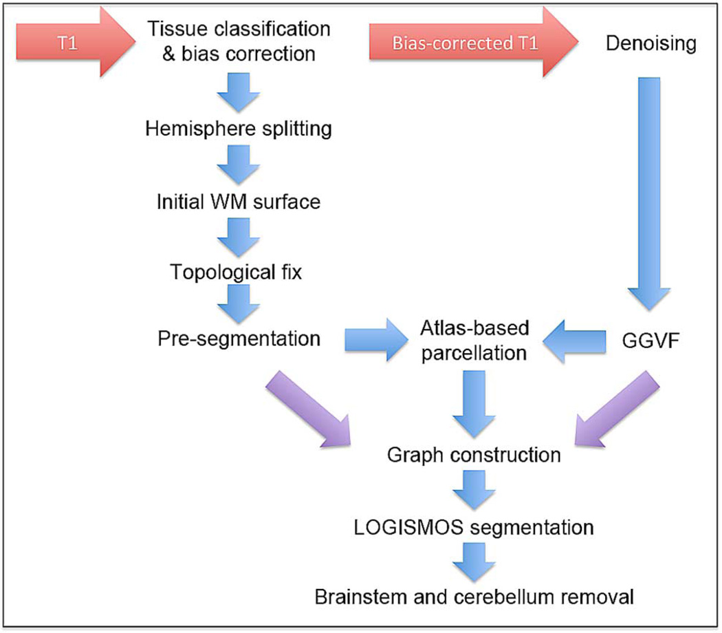
Our cortical segmentation method LOGISMOS-B1 consists of four main steps: 1) pre-processing of the raw input image to create a rough preliminary segmentation; 2) graph construction; 3) LOGISMOS segmentation; and 4) post-processing for removal of brain stem and cerebellum. An overview of the pipeline is given in Fig. 1.
Fig. 1.
Pipeline overview. The pre-processing creates an initial WM surface. This surface, as well as the GGVF method and the regional parcellation are combined together to construct a graph. LOGISMOS-based segmentation generates the final WM and GM surfaces. Finally, the brainstem and cerebellum are removed in post-processing.
A. Image Pre-Processing
The input to our algorithm is a single T1-weighted structural MR image. First, this T1w image is input to the BRAINSABC software2 [23] for pre-processing. BRAINSABC deformably registers the input image to an atlas and performs atlas-based tissue classification and bias-field correction using an expectation-maximization algorithm for simultaneous probabilistic tissue classification and bias-field correction [24]. This classification is limited to high-level tissue classes such as white matter (WM), gray matter (GM), cerebellar white, and gray matter, as well as nonbrain tissue types such as the skull.
All voxels that were classified as brain tissue (WM, GM, subcortical, etc.) are combined, and the resulting binary image is morphologically dilated using a spherical structuring element (r = 1 mm) to create a skull-strip mask. Next, the cerebral cortex is split into two hemispheres. This is done by detecting the plane of maximal symmetry, using the implementation in the BRAINS package. Note that performing the segmentation separately per hemisphere removes any complications that may arise from the interactions between the two hemispheres near the midsagittal plane.
The largest connected component of the WM tissue segmentation in each hemisphere is used as the preliminary segmentation for the LOGISMOS-based segmentation after two topological correction steps. The first step is to fill “holes” in the WM pre-segmentation such that its boundary only consists of the inner surface of the cortical ribbon. This means any “holes” in the white matter that would create additional boundaries, such as the subcortical structures and ventricles, are filled in. Next, handles are detected and removed following the methodology in [25], [26]. Briefly, this technique detects handles and removes them by either filling them in or cutting them apart, based on the route that modifies the least number of voxels. This creates a binary map of spherical topology, the boundaries of which form an approximation of the inner surface of the cortical ribbon.
B. Graph Construction
Given an approximate preliminary segmentation, the LOGISMOS approach [15] provides a framework for optimal segmentation of multiple interacting surfaces. This is achieved by modeling the problem as a complex geometric graph. With a properly-ordered multicolumn graph, the segmentation task has been shown to reduce to a V-weighted net surface search problem which can be efficiently solved.
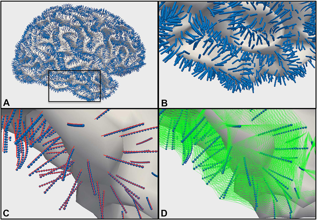
To this end, the preliminary segmentation is converted to a triangular mesh using the marching cubes algorithm. This mesh representation of the preliminary segmentation is referred to as the “base graph” in the LOGISMOS framework. From each node of this base graph (i.e., the vertices of the triangle mesh), a “column” is built, such that the final segmentation will “choose” exactly one node from each column. Consecutive nodes within a column are connected to each other by intra-column arcs. Nodes in neighboring columns are connected to each other by inter-column arcs, which introduce hard constraints on the smoothness of the final surface. Fig. 2 illustrates this graph structure.
Fig. 2.
Graph structure. (A) Whole WM surface (white) and the graph nodes (blue spheres). Black inset zoomed in (B), and further zoomed in the rest of panels. (C) Intra-column arcs (red) and graph nodes (blue). (D) Inter-column arcs (green) and graph nodes (blue).
The choice of method for building a single column of the geometric graph is crucial to the successful segmentation of complex objects such as the highly convoluted human cortex. We propose a new approach for building the columns of this geometric graph, based on the generalized gradient vector flows (GGVF [22]), which allow for spatially varying amount of smoothing based on the magnitude of the input gradient field. As discussed in detail in Section V-B, this technique is fundamental to the successful segmentation of the human cortex.
The gradient of the bias-field corrected T1-weighted image is computed, masked with the skull-strip mask and rescaled such that the maximum vector magnitude is equal to 1. This rescaled gradient field is used as the initial edge map in the following.
Given such an initial edge map f, the GGVF field v͂ is given by the equilibrium solution of
| (1) |
where g() and h() are the two weighting functions which govern the trade-off between the smoothing term and the data term. The smoothing term alone will produce a smoothly varying vector field. In contrast, the data term penalizes against large deviations from the input. The weighting functions are clearly dependent on the gradient of the edge map, which can be leveraged to reduce smoothing near strong gradients.
In practice, the recommended choice of weighting functions for GGVF are given by
| (2) |
| (3) |
In this setup, κ is the only remaining free parameter for controlling the amount of global smoothing.
As in [22], we implemented the partial differential equation specifying GGVF using an explicit finite difference scheme. Such an implementation has been shown to be numerically stable if the time step Δt is sufficiently small, specifically, if Δt ≤ (ΔxΔy)/(4gmax), where Δx and Δy are the spatial sample intervals and is the maximum value of the weighting function over the input edge map.
Once the GGVF field is computed, starting from each node in the base graph obtained from the preliminary segmentation, the graph columns are built by following the GGVF field using a step size Δ, which determines node spacing along a column.
Multiple surfaces are represented by introducing duplicates of this entire graph (base graph and the associated GGVF columns) and introducing inter-surface arcs which encode hard constraints on minimum and maximum surface separation. In the proposed method, we use the white matter surface (i.e., the WM-GM boundary) as the base graph, and both the WM surface and the pial surface (i.e., the GM-CSF boundary) are considered to be mutually interacting, nonintersecting surfaces of the same object. The surface separation constraints are set by considering the expected range of cortical thickness from the literature. Note that the two hemispheres are considered separately.
C. Regionally-Aware Segmentation
The gradient vector field (and its flow) are inherently better behaved near strong edges rather than inside regions of homogenous intensity. To minimize the effect of meaningless gradient directions on the graph construction in these flat regions, any nodes along a column that require more than 180 rotation of the gradient direction may typically be discarded. However, in certain thick parts of the cortex, such as the cingulate, the image intensity remains flat for a relatively long distance between the two gradient peaks corresponding to the WM and GM boundaries. Our heuristic for reducing noise may therefore prevent the desired GM boundary from being included in the search space.
However, removing this heuristic globally may result in zigzags in the columns as they travel through the flat intensity regions; these columns may intersect each other and potentially lead to self-intersecting surface segmentations. Instead, we introduce regional-awareness: in regions that are known a priori to have a thick cortical mantle, the exclusion heuristic is locally relaxed. The inter-column smoothness constraint is also relaxed in these regions as well as at the boundary of the region to allow for the graph behavior to change locally. This allows for accurate segmentation of the GM boundary in the cingulate and similarly thick regions, without adversely affecting the segmentation elsewhere.
The definitions of regions for this purpose is obtained using a registration-based approach. The BRAINSABC tissue classification software maps an external atlas to the subject image as part of the pre-processing stage. This mapping is used to carry the atlas labels to the subject space. Then, each graph column is assigned a label by considering the label at the pre-segmentation mesh vertex. However, the pre-segmentation mesh is not the final, accurate WM surface and is not guaranteed to lie on the cortex. If this vertex does not have a cortical label (i.e., it falls in a subcortical ROI), then we consider the label of a second node that corresponds to the minimum separation constraint between the two surfaces. Any graph columns that are still not assigned labels (e.g., because the second node falls outside the brain) are assigned via majority voting from the neighboring columns. Note that the goal is not to create a perfect parcellation, but rather to provide an estimate of the current region that can be used to adjust segmentation parameters locally.
The 35 ROIs defined in our atlas are, for each hemisphere, as follows: insula, anterior and posterior parts of middle frontal gyrus, cuneus, ambiens gyrus, fusiform gyrus, inferior parietal lobule, inferior temporal gyrus, isthmus of cingulate gyrus, lateral occipital gyrus, lateral orbital gyrus, lingual gyrus, straight gyrus, middle temporal gyrus, parahippocampal gyrus, paracentral lobule, opercular part of inferior frontal gyrus, orbital part of inferior frontal gyrus, triangular part of inferior frontal gyrus, visual cortex, postcentral gyrus, posterior cingulate gyrus, precentral gyrus, precuneus, caudal and rostral parts of anterior cingulate gyrus, superior frontal gyrus, superior parietal lobule, superior temporal gyrus, supramarginal gyrus, frontal pole, temporal pole, transverse temporal gyrus, limen insulae. These ROIs are illustrated in Fig. 3. The mapping on a typical subject is shown in Fig. 4.
Fig. 3.
Regional parcellation of the cortex for the atlas. Colors denote different ROIs. Left: Lateral view. Middle: Medial view. Right: Top view.
Fig. 4.
Regional parcellation of the cortex for a typical subject. Colors denote different ROIs. Left: Lateral view. Middle: Medial view. Right: Top view. Note that, because the parcellation is computed using the pre-segmentation surface, these are WM surfaces (unlike the atlas visualization in Fig. 3). Furthermore, note that the pre-segmentation surfaces contain brainstem and cerebellum, which are later removed in post-processing.
D. LOGISMOS Segmentation
Each node in the graph is assigned a cost related to the segmentation task such that a desirable segmentation has a low cost. Our cost function is based on edge strength, as defined by the first and second derivatives of image intensity [27]. Then, LOGISMOS finds the minimum closed set of this graph, which is equivalent to the minimum-cost cut or the optimal surface segmentation.
The bias corrected T1-weighted image is de-noised using gradient anisotropic diffusion filtering for five iterations using the ITK implementation with the default conductance value of 1. For the white matter surface, the gradient magnitude of the T1-weighted image is used as the cost function. For the gray matter surface, a weighted sum of the first and second order derivatives of the T1-weighted image is used, as given by the gradient magnitudes. Specifically
| (4) |
| (5) |
| (6) |
All gradients were computed via convolution with recursive Gaussians with a kernel size of σ = 0.2 mm. To account for different image intensity magnitudes and to simplify the weighting of these costs against each other, all gradient images (∇T1, ∇|∇T1|) are rescaled such that their intensity range is [0 … 1. The weight w was determined experimentally.
E. Mesh Post-Processing
LOGISMOS segmentation results contain varying amounts of brain stem and cerebellum tissue, which are removed via post-processing on the meshes. This is accomplished by creating a binary mask corresponding to the regions to be removed for each subject. To form the binary mask, cerebellar white and gray matter regions that resulted from BRAINSABC tissue classification during pre-processing are merged and morphologically closed to remove any present holes. The brain stem segmentation is obtained by mapping the atlas segmentation to the subject’s image using image registration also computed by BRAINSABC. The largest connected component in the brain stem segmentation is extracted and morphologically dilated to ensure full coverage of undesired mesh vertices. The brain stem and cerebellum segmentations thus obtained are combined together to create the binary mask to be used for post-processing. Each WM mesh vertex that falls within this mask and each corresponding GM vertex are removed. The mesh openings created in this process are closed with planar patches.
III. Experimental Methods
A. Data
To evaluate the performance of our algorithm, we used the cortical reconstruction validation resource from Johns Hopkins University3. This validation dataset contains volumetric T1w and FLAIR MR images of multiple sclerosis (MS) patients and healthy controls [28]. For the experiments presented in this paper, only the T1-weighted images were used. The images of the healthy controls have an isotropic resolution of (1 mm)3 while the images of the MS patients have an isotropic resolution of (0.83 mm)3. Additionally, the dataset includes manually picked landmark points in seven different regions of the cortex on both inner and outer surfaces, identified by two independent raters. Each of these seven regions (calcarine sulcus, cingulate, central sulcus, parieto-occipital sulcus, superior-frontal sulcus, superior-temporal sulcus, and the Sylvian fissure) have 30 landmarks per hemisphere, referred to as clusters in the following. Therefore, 7 clusters × 2 hemispheres × 2 surfaces × 30 landmarks × 2 raters = 1680 landmarks are available per subject, for a total of 16 800 manual landmarks for 10 subjects (five MS, five healthy controls). The MS subjects have additional landmark clusters picked in the vicinity of white matter lesions. Not relevant to our cortical surface segmentation task, these additional landmarks were not used in the evaluation.
B. Compared Methods
Considering that FreeSurfer currently represents the state-of-the-art approach, we have compared our algorithm with FreeSurfer. In particular, we have used the 5.1 release version of FreeSurfer and used the first two steps of the automated reconstruction pipeline (skull-stripping and cortical reconstruction). In order to isolate the provenance of performance differences, we have investigated a hybrid method that consisted of skull-stripping using the LOGISMOS-B method followed by FreeSurfer reconstruction.
For our algorithm, we have used the following parameter settings. For the preliminary segmentation, the BRAINSABC software was used; this included three iterations of gradient anisotropic diffusion filtering as pre-processing, followed by a symmetric diffeomorphic registration using a 10 × 10 × 10 grid. The atlas distributed with the BRAINS package was used for tissue classification and regional parcellation. For GGVF, we used κ = 0.05 and five iterations.
For the graph construction, we used 20 000 columns containing 120 nodes each, with a node spacing of 0.1 mm for each hemisphere. The inter-surface separation constraints were set to a minimum of 2.5 mm and a maximum of 15 mm (i.e., no maximum was enforced in practice). The gray matter cost function had the weighting parameter w = 0.75. The cingulate (caudal and rostral parts of anterior cingulate gyrus) and the temporal gyrus (transverse temporal gyrus and superior temporal gyrus) exhibit markedly thicker gray matter layer than other brain regions and were therefore extracted from the parcellation for the purpose of regionally-aware segmentation. These ROIs were enlarged by propagating them (via nearest neighbor) for 10 iterations. The inter-column smoothness constraint was set at an interval of 1 node outside the chosen ROIs, two nodes inside the chosen ROIs and eight nodes at the ROI-non_ROI interface to allow local behavior change. The node exclusion threshold was set using vector inner product of local GGVF direction between consecutive nodes; the threshold was 0 (equivalent to 180 rotation) outside the ROIs and −0.1 inside the ROIs.
C. Evaluation Criteria
For each manual landmark, we compute its signed and unsigned distance to the reconstructed surface. In order to create a single independent standard, the landmarks from the two experts were pooled together and surface distances were obtained by averaging of cluster-specific distances over all landmarks from both sets. The hemisphere and inner/outer surface location of each cluster is provided, which makes it possible to use the appropriate surface in the computation (left/right WM/GM). The distance is computed by locating the closest triangle on the mesh using an octree-based search method and then computing the distance between the landmark and this triangle. Note that the distance is measured between the landmark and the closest point on the triangle, which may or may not coincide with a vertex. In order to determine the sign of the distance, the surface mesh was scan-converted into a high resolution binary image (0.5 × 0.5 × 0.5 mm3), which was used as an efficient lookup table to determine whether a landmark is inside or outside the surface. Note that the binary lookup was used only for the inside/outside decision; the actual distances were measured directly as point-to-surface distances.
We report the average landmark-surface distance for each landmark cluster as well as for the entire dataset. Additionally, we also report computation times for each method. Two-tailed paired t-tests were used for statistical comparison, with 0.05 significance threshold.
IV. Results
The unsigned GM errors were quite similar between FreeSurfer and LOGISMOS-B (p = 0.44) but LOGISMOS-B had significantly smaller WM unsigned error (p = 0.05). However, the hybrid approach had significantly worse results than both FreeSurfer (p = 0.02 for WM and p ≪ 0.001 for GM) and LOGISMOS-B (p = 0.01 for WM and p = 0.08 for GM).
LOGISMOS-B had significantly smaller signed errors for both the white matter (p ≪ 0.001) and the gray matter (p ≪ 0.001) compared to both FreeSurfer and the hybrid approach. The WM signed error was not significantly different between the FreeSurfer and hybrid approaches (p = 0.420); while the GM signed error was significantly larger for the hybrid approach (p ≪ 0.001).
Table I–VI summarize the quantitative comparisons of the individual methods. Note that since the hybrid approach delivered an overall inferior performance, the statistical significance assessments of differences presented in all the Tables are limited to the pairwise comparisons between the LOGISMOS-B and FreeSurfer methods.
TABLE I.
Mean and Standard Deviation of Unsigned Distance Between Manual Landmarks and Reconstructed Cortical Surfaces.
| Avg. unsigned error (mm) | LOGISMOS-B | FreeSurfer | Hybrid |
|---|---|---|---|
| White matter | *0.575 ± 0.255 | 0.611 ± 0.302 | 0.627 ± 0.332 |
| Gray matter | 0.684 ± 0.300 | 0.703 ± 0.331 | 0.730 ± 0.349 |
Asterisks Indicate Statistically Significant Differences. Statistical Comparison Only Between LOGISMOS-B and FreeSurfer
TABLE VI.
Mean and Standard Deviation of Distance Between Manual Landmarks and Reconstructed Cortical Surfaces, for Healthy Subjects and MS Patients.
| Avg. error (mm) | Healthy | MS | ||
|---|---|---|---|---|
| LOGISMOS-B | FreeSurfer | LOGISMOS-B | FreeSurfer | |
| Siqned WM error | 0.122 ± 0.431 | 0.161 ± 0.485 | *0.046 ± 0.439 | 0.366 ± 0.392 |
| Signed GM error | −0.072 ± 0.604 | 0.053 ± 0.478 | *0.088 ± 0.358 | −0.388 ± 0.542 |
| Unsigned WM error | *0.580 ± 0.255 | 0.675 ± 0.250 | 0.571 ± 0.256 | 0.546 ± 0.336 |
| Unsigned GM error | 0.777 ± 0.348 | *0.644 ± 0.234 | *0.592 ± 0.206 | 0.762 ± 0.397 |
Asterisks Indicate Statistically Significant Differences Between LOGISMOS-B and FreeSurfer
Table I and Table II compare the unsigned and signed errors for LOGISMOS-B, FreeSurfer, and the hybrid approach.
TABLE II.
Mean and Standard Deviation of Signed Distance Between Manual Landmarks and Reconstructed Cortical Surfaces.
| Avg. signed error (mm) | LOGISMOS-B | FreeSurfer | Hybrid |
|---|---|---|---|
| White matter | *0.084 ± 0.436 | 0.263 ± 0.452 | 0.271 ± 0.478 |
| Gray matter | *0.008 ± 0.502 | −0.167 ± 0.556 | −0.212 ± 0.579 |
Asterisks Indicate Statistically Significant Differences. Statistical Comparison Only Between LOGISMOS-B and FreeSurfer
Table III and Table IV show the average signed and unsigned errors per cluster, respectively. Bonferroni correction was used to address multiple comparisons in this analysis, with n = 56 (two types of distances ×14 clusters ×2 surfaces).
TABLE III.
Signed Distance Between Manual Landmarks and Reconstructed Cortical Surfaces, Broken Down by Sulcus.
| Signed error (mm) | LCALC | LCING | LCS | LPO | LSF | LST | LSYL | RCALC | RCING | RCS | RPO | RSF | RST | RSYL | Overall | |
|---|---|---|---|---|---|---|---|---|---|---|---|---|---|---|---|---|
| WM | LOGISMOS-B | −0.39 | 0.20 | **−0.12 | −0.01 | *0.34 | 0.13 | 0.14 | −0.27 | *0.60 | −0.20 | 0.14 | 0.40 | 0.17 | 0.02 | **0.084 |
| FreeSurfer | −0.32 | 0.30 | 0.46 | 0.03 | 0.50 | 0.24 | 0.17 | *0.24 | 0.96 | 0.02 | 0.19 | 0.49 | 0.27 | 0.12 | 0.263 | |
| Hybrid | −0.40 | 0.30 | 0.45 | 0.02 | 0.53 | 0.31 | 0.15 | 0.27 | 0.93 | 0.01 | 0.28 | 0.50 | 0.27 | 0.12 | 0.271 | |
| GM | LOGISMOS-B | −0.38 | −0.06 | 0.04 | *0.04 | 0.21 | *0.03 | *0.07 | −0.23 | 0.42 | −0.14 | 0.26 | 0.17 | 0.00 | −0.29 | **0.008 |
| FreeSurfer | −0.34 | −0.25 | −0.28 | −0.31 | −0.22 | −0.32 | −0.22 | −0.07 | 0.24 | −0.34 | *0.03 | −0.03 | 0.07 | −0.31 | −0.167 | |
| Hybrid | −0.40 | −0.27 | −0.31 | −0.34 | −0.27 | −0.31 | −0.33 | −0.06 | 0.18 | −0.44 | 0.03 | −0.09 | −0.04 | −0.30 | −0.212 |
Single Asterisk Indicates Statistically Significant Difference in the Raw Data
Double Asterisk After Multiple Comparison Correction
Statistical Comparison Only Between LOGISMOS-B and FreeSurfer. L—Indicates Left Hemisphere, R—Indicates Right Hemisphere. CALC: Calcarine Sulcus, CING: Cingulate, CS: Central Sulcus, PO: Parieto-Occipital Sulcus, SF: Superior-Frontal Sulcus, ST: Superior-Temporal Sulcus, SYL: Sylvian Fissure
TABLE IV.
Unsigned Distance Between Manual Landmarks and Reconstructed Cortical Surfaces, Broken Down by Sulcus.
| Unsigned error (mm) | LCALC | LCING | LCS | LPO | LSF | LST | LSYL | RCALC | RCING | RCS | RPO | RSF | RST | RSYL | Overall | |
|---|---|---|---|---|---|---|---|---|---|---|---|---|---|---|---|---|
| WM | LOGISMOS-B | 0.89 | 0.55 | 0.64 | 0.50 | *0.46 | *0.51 | *0.56 | 0.73 | *0.74 | 0.64 | 0.44 | *0.53 | 0.38 | 0.50 | *0.575 |
| FreeSurfer | 0.80 | 0.57 | 0.48 | 0.53 | 0.58 | 0.65 | 0.68 | 0.69 | 1.02 | *0.44 | 0.52 | 0.65 | 0.49 | 0.46 | 0.611 | |
| Hybrid | 0.80 | 0.58 | 0.47 | 0.54 | 0.61 | 0.73 | 0.67 | 0.75 | 1.01 | 0.44 | 0.58 | 0.67 | 0.47 | 0.46 | 0.627 | |
| GM | LOGISMOS-B | 0.80 | 0.79 | **0.50 | *0.56 | *0.59 | *0.68 | 0.77 | 0.68 | 0.93 | *0.52 | 0.53 | 0.72 | 0.65 | 0.84 | 0.684 |
| FreeSurfer | 0.71 | 0.71 | 0.86 | 0.77 | 0.90 | 0.87 | 0.75 | *0.52 | **0.46 | 0.74 | 0.55 | 0.79 | 0.57 | 0.70 | 0.703 | |
| Hybrid | 0.72 | 0.74 | 0.87 | 0.79 | 0.93 | 0.91 | 0.75 | 0.57 | 0.48 | 0.82 | 0.55 | 0.82 | 0.58 | 0.70 | 0.730 |
Single Asterisk Indicates Statistically Significant Difference in the Raw Data
Double Asterisk After Multiple Comparison Correction
Statistical Comparison Only Between LOGISMOS-B and FreeSurfer. L—Indicates Left Hemisphere, R—Indicates Right Hemisphere. CALC: Calcarine Sulcus, CING: Cingulate, CS: Central Sulcus, PO: Parieto-Occipital Sulcus, SF: Superior-Frontal Sulcus, ST: Superior-Temporal Sulcus, SYL: Sylvian Fissure
Table V compares the average run times for FreeSurfer and LOGISMOS-B. LOGISMOS-B can be seen to be more than three times faster than FreeSurfer (p ≪ 0.001). In particular, the atlas-based tissue classification took 139 min, the hemisphere splitting 23 min, the topological correction 2 min, the graph segmentation 8 min, and mesh post-processing less than a minute on average.
TABLE V.
Computation Times for FreeSurfer and LOGISMOS-B Cortical Reconstruction.
| FreeSurfer | LOGISMOS-B | |
|---|---|---|
| Average run time (hh:mm) | 9:58 | *2:55 |
Asterisks Indicate Statistically Significant Differences
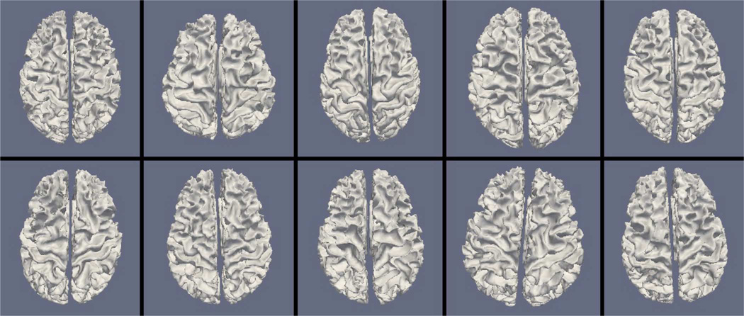
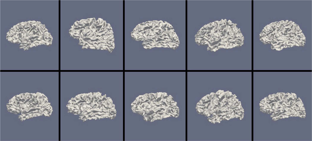
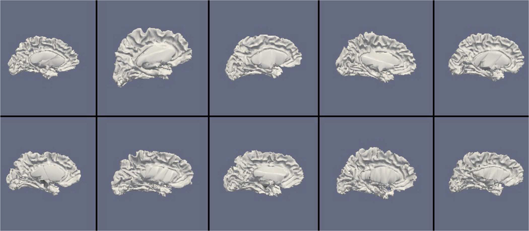
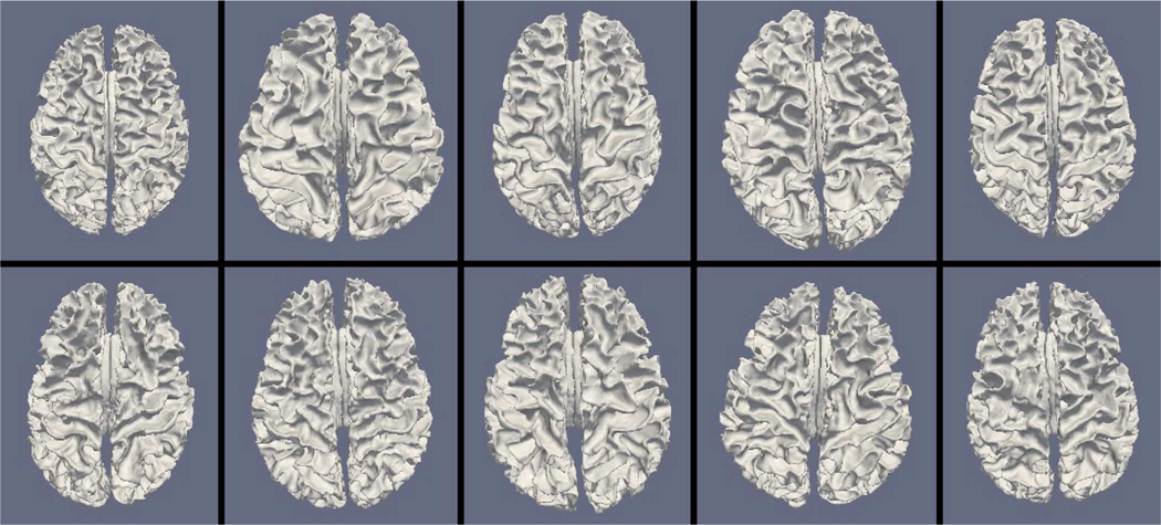
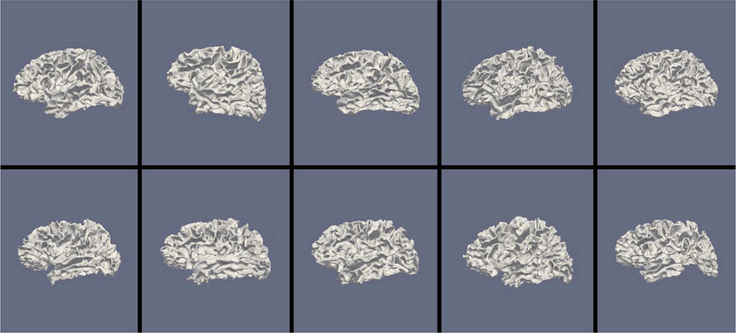
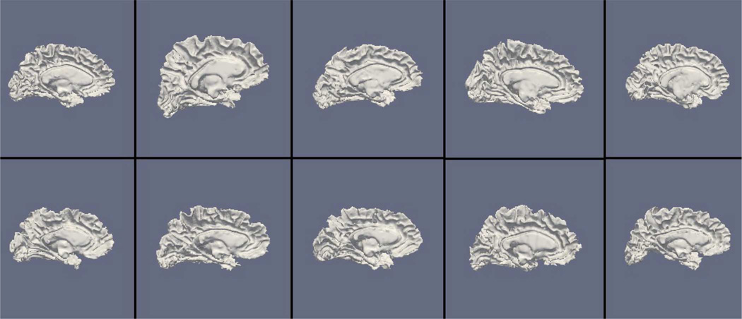
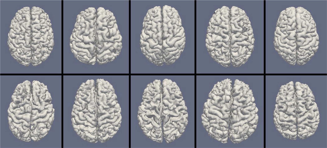
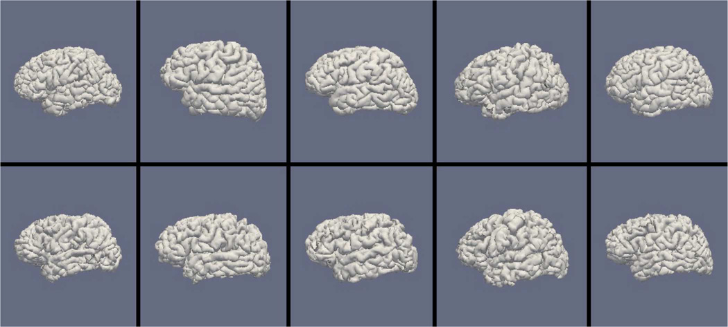
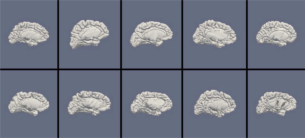
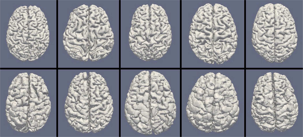
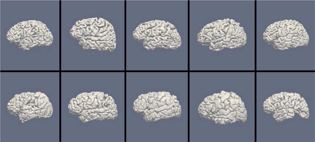
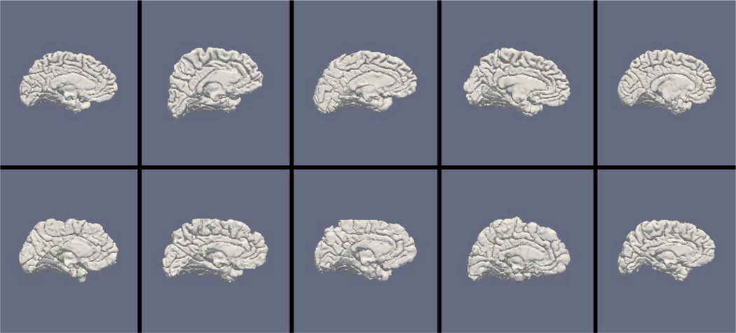
Figs. 9, 11, and 13 show the 10 reconstructed LOGISMOS-B white matter surfaces from the top, side, and medial views, while Figs. 10, 12, and 14 show the corresponding FreeSurfer results. Similarly, Figs. 15, 17, and 19 show the 10 reconstructed LOGISMOS-B gray matter surfaces, and Figs. 16, 18, and 20 show the corresponding FreeSurfer results. Again, the performance of the two approaches for the healthy subjects are comparable, whereas the differences are quite noticeable for the MS patients. Table VI summarizes the surface errors per healthy/MS subject groups and statistical significance of their differences for LOGISMOS-B and FreeSurfer.
Fig. 9.
Reconstructed white matter surfaces for 10 subjects with LOGISMOS-B, top view. Top row: Healthy controls. Bottom row: MS patients.
Fig. 11.
Reconstructed white matter surfaces for 10 subjects with LOGISMOS-B, side view. Top row: Healthy controls. Bottom row: MS patients.
Fig. 13.
Reconstructed white matter surfaces for 10 subjects with LOGISMOS-B, medial view. Top row: Healthy controls. Bottom row: MS patients.
Fig. 10.
Reconstructed white matter surfaces for 10 subjects with FreeSurfer, top view. Top row: Healthy controls. Bottom row: MS patients.
Fig. 12.
Reconstructed white matter surfaces for 10 subjects with FreeSurfer, side view. Top row: Healthy controls. Bottom row: MS patients.
Fig. 14.
Reconstructed white matter surfaces for 10 subjects with FreeSurfer, medial view. Top row: Healthy controls. Bottom row: MS patients.
Fig. 15.
Reconstructed gray matter surfaces for 10 subjects with LOGISMOS-B, top view. Top row: Healthy controls. Bottom row: MS patients.
Fig. 17.
Reconstructed gray matter surfaces for 10 subjects with LOGISMOS-B, side view. Top row: Healthy controls. Bottom row: MS patients.
Fig. 19.
Reconstructed gray matter surfaces for 10 subjects with LOGISMOS-B, medial view. Top row: Healthy controls. Bottom row: MS patients.
Fig. 16.
Reconstructed gray matter surfaces for 10 subjects with FreeSurfer, top view. Top row: Healthy controls. Bottom row: MS patients.
Fig. 18.
Reconstructed gray matter surfaces for 10 subjects with FreeSurfer, side view. Top row: Healthy controls. Bottom row: MS patients.
Fig. 20.
Reconstructed gray matter surfaces for 10 subjects with FreeSurfer, medial view. Top row: Healthy controls. Bottom row: MS patients.
V. DISCUSSION
A. Performance
The presented results indicate that LOGISMOS-B is an accurate method for automated determination of the human cortical surface. While the performance difference for unsigned GM surface positioning errors did not reach statistical significance between the LOGISMOS-B and FreeSurfer approaches, the WM unsigned errors were significantly smaller for LOGISMOS-B. Additionally, LOGISMOS-B exhibited significantly smaller signed surface positioning errors than FreeSurfer, both for the WM and the GM surfaces, showing a significantly smaller inside/outside positioning bias of both the GM and WM cortical surfaces. This improved accuracy can at least partially be attributed to the fact that LOGISMOS-B is guaranteed to find the globally optimal solution, whereas FreeSurfer is subject to local minima during its gradient-based optimization process.
The breakdown of surface positioning errors into clusters, presented in Table III and Table IV, gives further insight into the performance of LOGISMOS-B. It can be seen that for some regions, such as the parieto-occipital sulcus, surface localization is highly accurate. In some other regions, such as the cingulate, the localization shows lower levels of accuracy, especially for the GM surface. This may be partially explained by imperfect splitting of the hemispheres during the pre-processing by the BRAINS package. The use of regionally-aware segmentation improves LOGISMOS-B’s performance considerably in this region, while other regions are unaffected, as expected. Further improvement may be possible by introducing regional cost functions to capture local characteristics of the brain, again by leveraging the possibility of the regionally-aware segmentation approach in LOGISMOS-B. Note that, given the high number of comparisons, the best approach somewhat varies per region, as to be expected; however, overall, LOGISMOS-B offers the best performance.
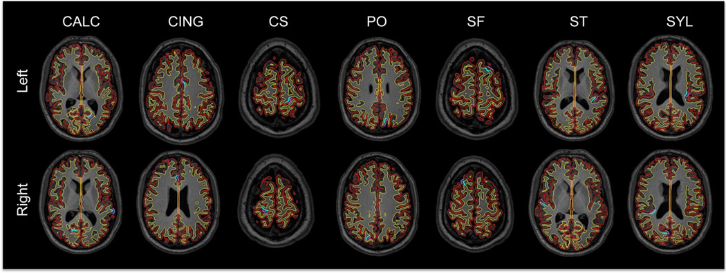
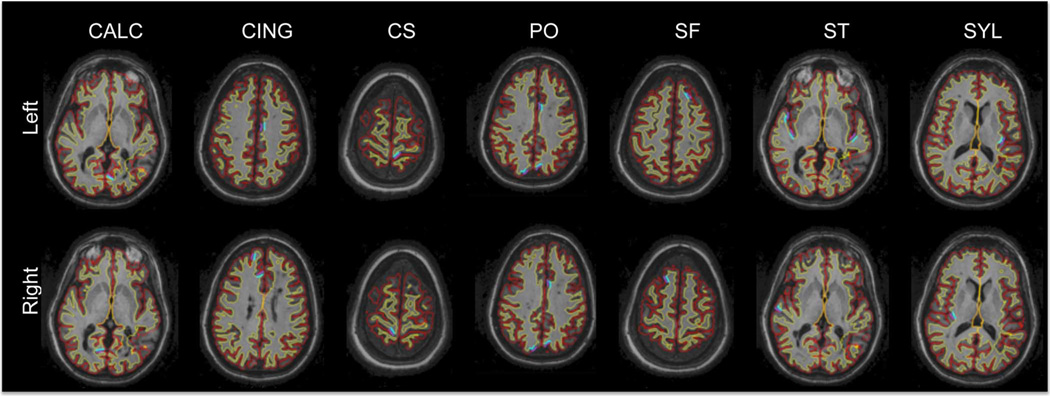
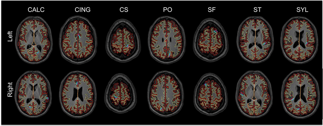
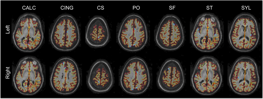
It can be observed from both quantitative and qualitative results that LOGISMOS-B performs very well not only in normal brains but also in MS patients, despite not being specifically adapted to the presence of lesions (unlike approaches such as [28] which explicitly segment the MS lesions before cortical reconstruction). This is due to the underlying LOGISMOS framework which yields a globally optimal solution and is therefore extremely robust with respect to both the image noise and the presence of lesions. LOGISMOS is insensitive to local minima of the energy functional and LOGISMOS-B is further helped by employment of GGVF columns that help recovery from imperfect preliminary segmentations as discussed below. The 3-D figures (Figs. 9–20) clearly demonstrate the robustness of LOGISMOS-B in comparison to the FreeSurfer approach for the MS patients. In particular, note the fused gyri throughout the brain for most if not all MS patients using the FreeSurfer approach. Additionally, note the missing folds near the postcentral gyrus for the second MS patient and the very large chunk of tissue entirely missing near the inferior temporal gyrus for the fifth MS patient (best visible on Fig. 18). The 2-D figures (Figs. 5–8) also clearly show these missing tissues in the FreeSurfer segmentations for MS subjects (best visible for the slices corresponding to the left CALC and ST on Fig. 8). These faulty segmentations often happen in the neighborhood of an MS lesion, which creates local minima for the energy functional of the FreeSurfer optimization, by introducing strong edges locally and by causing the tissue appearance to deviate from the expected intensity profiles. The graph-based segmentation underlying the LOGISMOS-B approach guarantees finding the global optimum with respect to the employed cost function [29] and is therefore inherently more robust against such local minima. Both the qualitative and quantitative results indicate that the performance of LO-GISMOS-B and FreeSurfer is comparable for the healthy subjects, with LOGISMOS-B giving slightly more accurate results for the WM surface and FreeSurfer giving slightly more accurate results for the GM surface. The excellent performance of LOGISMOS-B in both populations suggests it is suitable for use in a variety of datasets.
Fig. 5.
Outline of the reconstructed LOGISMOS-B surfaces on a series of horizontal slices for a healthy subject. Red: GM surface, yellow: WM surface. Manually picked landmark clusters are shown in purple (GM) and blue (WM). CALC: Calcarine sulcus, CING: cingulate, CS: central sulcus, PO: parieto-occipital sulcus, SF: superior-frontal sulcus, ST: superior-temporal sulcus, SYL: Sylvian fissure.
Fig. 8.
Outline of the reconstructed FreeSurfer surfaces on a series of horizontal slices for an MS patient. Red: GM surface, yellow: WM surface. Manually picked landmark clusters are shown in purple (GM) and blue (WM). CALC: Calcarine sulcus, CING: cingulate, CS: central sulcus, PO: parieto-occipital sulcus, SF: superior-frontal sulcus, ST: superior-temporal sulcus, SYL: Sylvian fissure.
Note also the left–right symmetry of the presented results using LOGISMOS-B, which can be observed both visually as well as from the similar patterns in the error measurements between the hemispheres. This observed symmetry is a further evidence of LOGISMOS-B cortical surface segmentation accuracy.
Signed and unsigned distances to landmarks measure different properties of the methods. A high signed error indicates a systematic over- or under- segmentation bias. Even though individual landmarks may have large errors, they have to “cancel” each other out to achieve a low average signed error, which would indicate the surface is, on average, at the correct location. On the other hand, the unsigned error represents the aggregated local errors regardless of their directions—as such, they never cancel each other. For small overall signed distance errors, it can be interpreted as the variability of the signed distance. While achieving close-to-zero unsigned errors is impossible without achieving close-to-zero signed errors, the opposite is not true. Specifically, once a close-to-zero bias is achieved (close-to-zero signed positioning errors), it is desirable to demonstrate that the unsigned errors are also small showing low variations of the segmented surfaces around the independent standard. Our results indicate that, LOGISMOS-B has a very small segmentation bias and low unsigned errors. The achieved error rates demonstrate a performance improvement compared to that of the FreeSurfer.Figs. 5 and 6 show the original MR image for a healthy subject with the reconstructed surfaces as mesh cross sections with a series of horizontal slices, for LOGISMOS-B and FreeSurfer, respectively. The manual landmarks from one expert are shown overlaid on the images. The most superior slice was chosen from each cluster. Figs. 7 and 8 show the same for an MS patient. The performance of the two approaches for the healthy subject is comparable, whereas the differences are quite noticeable for the MS patient.
Fig. 6.
Outline of the reconstructed FreeSurfer surfaces on a series of horizontal slices for a healthy subject. Red: GM surface, yellow: WM surface. Manually picked landmark clusters are shown in purple (GM) and blue (WM). CALC: Calcarine sulcus, CING: cingulate, CS: central sulcus, PO: parieto-occipital sulcus, SF: superior-frontal sulcus, ST: superior-temporal sulcus, SYL: Sylvian fissure.
Fig. 7.
Outline of the reconstructed LOGISMOS-B surfaces on a series of horizontal slices for an MS patient. Red: GM surface, yellow: WM surface. Manually picked landmark clusters are shown in purple (GM) and blue (WM). CALC: Calcarine sulcus, CING: cingulate, CS: central sulcus, PO: parieto-occipital sulcus, SF: superior-frontal sulcus, ST: superior-temporal sulcus, SYL: Sylvian fissure.
While the data presented here only used T1-weighted images for a fair comparison with FreeSurfer, our framework can be readily adapted to work with multiple magnetic resonance imaging (MRI) contrasts. For example, if T2-weighted images are available, they can be used for improved GM surface segmentation by including the gradient of the T2-weighted image in the cost function. Additionally, it may be possible to improve the preliminary segmentation by using both images for tissue classification. Using multiple images would naturally slow down the computation time, especially for the tissue classification step. The LOGISMOS-based segmentation step creates a single cost function, whether based on a single T1-weighted image or a pair of T1w and T2w images; therefore, the additional computational load would be limited to the cost function computation step. In our experience, using a secondary input image increases the computation time of the tissue classification time linearly, whereas the LOGISMOS-based segmentation step computation time remains in roughly the same order of magnitude. Additionally the increased accuracy of the preliminary tissue classification may not justify the extra computational load, since the subsequent LOGISMOS-based segmentation step is designed to improve the preliminary segmentation and it was shown to successfully recover from errors in the input.
The results of the hybrid approach offer interesting insight into the source of the performance differences. One possible explanation would be that LOGISMOS-B simply uses a better skull-stripping technique. To test this hypothesis, we created the hybrid approach that uses the LOGISMOS-B skull-strip mask to bypass the FreeSurfer pre-processing. Remarkably, this method performs worse than both FreeSurfer and LOGISMOS-B, on all accounts. The fact that the hybrid approach performs worse than LOGISMOS-B clearly shows that the performance improvement that LOGISMOS-B enjoys is not a trivial side effect of better pre-processing. Furthermore, the lower accuracy of the hybrid approach compared to FreeSurfer implies that the skull-stripping technique used in LOGISMOS-B may in fact be less accurate than that used in the FreeSurfer approach. We note that this result is somewhat expected because LOGISMOS-B pre-processing does not aim to achieve perfect or optimal skull-stripping; it merely aims to provide the most suitable input to the segmentation stage. This means an overly conservative estimate of the mask: the robust LOGISMOS-based segmentation can readily recover from an overly inclusive skull-strip mask, but it can not recover from a too aggressive strip. Additionally, due to our need for a pre-segmentation, we favor an approach that provides a rough white matter mask in addition to the skull-strip mask. Importantly, this emphasizes that we do not propose an alternative to just the segmentation component of FreeSurfer but to the entire FreeSurfer pipeline. Our results demonstrate that our pipeline as a whole leads to a more accurate segmentation than the FreeSurfer pipeline as a whole.
B. Construction of Graph Columns
The choice of method for building a single column of the geometric graph is crucial to the successful segmentation of complex objects such as the highly convoluted human cortex and is at the core of LOGISMOS-B. For convex surfaces, using equally spaced nodes along the surface normal direction offers an adequate solution. For nonconvex surfaces, however, these normal lines intersect, potentially leading to a self-intersecting surface segmentation. One approach to solve this problem involves the concept of electric lines of force (ELF) [29], which are theoretically guaranteed not to intersect each other. However, the computation of the ELF direction at any given point requires the computation of distances to all vertices, which is computationally prohibitive for dense meshes. In practice, the ELF computation can be limited to a local neighborhood, which works well for surfaces of limited curvature but no longer offers the theoretical nonself-intersection guarantee that is present in the general case. A recent approach [30] uses dynamic particle systems to compute layers of sample points around the base graph. While this approach was shown to work well for simple shapes, it does not guarantee nonself-intersection in the complex setting of the cortical surface.
Bauer et al. [31] propose using gradient vector flows (GVF) to overcome this problem. They compute the gradient image of the binary preliminary segmentation to create an initial gradient field, which is then “flowed” using the gradient vector flow (GVF) method [32] to create a smoothly varying vector field. The integral lines of this vector field are used to build the graph columns. While this approach guarantees nonoverlapping columns, the GVF force field is known to have difficulties near thin, long structures, which proves troublesome for the thin, deep sulcal folds of the human cortex. The gradient vector flow method [32] was originally developed to address the issue of poor convergence to boundary concavities in the context of snake-based segmentation. This method computes the diffusion of the gradient vectors from an initial edge map derived from an input image. The GVF field v͂ is given by the equilibrium solution of
| (7) |
where is the initial edge map and is a regularization parameter that controls the amount of smoothing performed by the flow. While GVF performs adequately for creating a smooth vector field that captures boundary concavities, it is nonetheless prone to problems near thin, elongated structures which tend to get overly smoothed.
For this reason, Xu et al. [22] later introduced the generalized GVF, or GGVF, which allows for a spatially varying amount of regularization. This is the variant we are using in LOGISMOS-B. Note that in the case of GVF, g(∇f|) = µ is a constant, which leads to indiscriminate smoothing everywhere in the image, while h(|∇f|) = |∇f|2 has a strong response near edge locations. As discussed in [22], when two edges are in close proximity, GVF tends to smooth between the edges and lose thin features these edges may represent, whereas the GGVF formulation leads to reduced smoothing (smaller g) in such regions and preserves thin features. This property is crucial in the cortical surface, since the entire cortical ribbon presents a dense edge field thanks to the sulcal folds.
Fig. 21 illustrates the different column building strategies. Using the normal directions [Fig. 21(A), (D), (G)] results in straight paths for the graph columns, which is clearly inappropriate for the highly folded cortical surface. The curved paths of ELF [Fig. 21(B), (E), (H)] offer substantial improvement over the normal directions. However, they may intersect each other after they pass the medial surface of the object, leading to self-intersecting final segmentations; this can be prevented by forcing them to stop at the medial surface, but this may cause them to pile up in certain regions and leave other regions under-sampled. Additionally, they are dependent on the preliminary segmentation. The proposed method based on the GGVF approach [Fig. 21(C), (F), (I)] yields nonoverlapping paths that converge to the medial surface while providing more regular coverage of the space.
Fig. 21.
Construction of graph columns. (A)–(C) Whole brain; (D)–(F) zoomed in view; (G)–(I) zoomed in view with cross-sectional clipping for illustrating the interior of the surface. Outside of the WM surface is shown in white, the inside in green, the graph columns in red.
Our approach offers two significant advantages over existing methods. First, the spatially varying smoothing allows the capture of thin long structures more effectively than the standard GVF approach. Second, using the gradient field of the grayscale image as the input vector field allows for decoupling the graph construction from the preliminary segmentation to a large extent. While the base graph is still dependent on the preliminary segmentation, the paths of the graph columns become independent of the preliminary segmentation. This is crucial for successful recovery from a poor preliminary segmentation. Even if a sulcus is entirely missing from the preliminary segmentation, the LOGISMOS stage can, at least in theory, fully recover it when using a graph constructed with this approach.
Note that the modications to LOGISMOS are a very signicant extension; without this methodological innovation, LOGISMOS performs extremely poorly for cortical reconstruction. For example, for the same dataset, using the same parameters but switching to ELF-based columns as in the original LOGISMOS framework, the segmentation fails frequently, and the signed errors are at the level of 2 mm for some regions. Visual inspection of the results also reveals that not only are the surfaces incorrectly placed in many regions, they also contain severe topological defects. The (sparse) ELF-based construction can not guarantee nonintersecting graph columns in the tightly folded cortex; this makes the smoothness and surface separation constraints impossible to enforce (since the columns do not satisfy the basic assumptions of ordering). The resulting surfaces therefore often intersect each other as well as self-intersect and are simply drawn to strong edges in the image regardless of the satisfaction of basic requirements for a good cortical reconstruction. In other words, while a multi-surface graph search serves as the underlying mechanism for both the original LOGISMOS and the reported LOGISMOS-B methods, the novel graph construction aspects presented here are responsible for the difference between a success and a failure when applied to the tightly folded GM/WM cortical surfaces imaged by MRI.
C. Preliminary Segmentation
An important concern is the choice of method for obtaining the preliminary segmentation. While the accuracy of this segmentation is not crucial to the final result, its topological correctness greatly affects the quality of the resulting mesh. In particular, any holes or handles that may be present in the preliminary segmentation lead to “runaway” graph columns that typically result in self-intersecting meshes. While it may be possible to remove such artifacts in post-processing, it is desirable to prevent them in the first place as much as possible, because they may cause inaccurate segmentation in their local neighborhoods. For this reason, we constrain the preliminary segmentation to only include the inner boundary of the cortex and remove any “holes” such as the subcortical structures. Note that imperfect preliminary segmentation of these may potentially lead to the final segmentation leaking into the subcortical structures. In addition to the subcortical structures, we also remove any artificial holes and handles that may result from inadequate spatial resolution. Our results indicate that the final meshes from our segmentations are largely free of intersections, except in the vicinity of the brainstem where the GM surface becomes ill-defined.
D. Algorithm Parameters
LOGISMOS-B has relatively few free parameters, and most of the parameters are related to the preliminary segmentation. For these, we have found that the default values provided in the BRAINS AutoWorkup suite are extremely robust and work well out-of-the-box.
The remaining parameters are with respect to the LOGISMOS segmentation, and have intuitive meaning. The number of columns and node spacing determine the level of detail in the final segmentations. The column height should be set large enough to ensure the desired solution is within the search space. The inter-surface separation constraints can be set based on expected range of cortical thickness.
The main parameter of cost function specification is the weight for the gray matter cost function. This parameter determines the ratio of the contribution of the first and second derivatives. Note that this parameter can be used to slightly move the GM segmentation inward or outward by favoring either the first derivative, which has strong response in the peak of the T1w intensity edge, or the second derivative, which has strong response inside and outside the peak of the first derivative [27].
E. Future Work
Considering the two hemispheres as two mutually interacting objects (with two surfaces each, i.e., WM and GM) may improve the behavior of the graph cut near the midsagittal plane, potentially increasing accuracy in regions such as the cingulate cortex.
One of the end goals of cortical surface reconstruction algorithms is to provide locally accurate measurements of cortical thickness. Expanding LOGISMOS-B to allow such analysis remains future work.
VI. Conclusion
The reported cortical reconstruction algorithm, LOGISMOS-B, is based on probabilistic tissue classification, generalized gradient vector flows and the LOGISMOS graph segmentation framework. Compared to the current state-of-the-art, LOGISMOS-B offers improved anatomic accuracy and dramatically reduced computational requirements.
Acknowledgment
This work was supported by the National Institutes of Health (NIH) National Institute of Biomedical Imaging and Bioengineering (NIBIB) under Grant R01-EB004640.
The authors would like to thank J. Prince and P. Calabresi for providing the image dataset and the independent standard [28].
Footnotes
B for Brain
Available online: https://github.com/BRAINSia/BRAINSTools
Contributor Information
Ipek Oguz, Email: ipek-oguz@uiowa.edu, Department of Electrical and Computer Engineering, The University of Iowa, Iowa City, IA 52242 USA.
Milan Sonka, Department of Electrical and Computer Engineering, The University of Iowa, Iowa City, IA 52242 USA.
References
- 1.Dale AM, Fischl B, Sereno MI. Cortical surfacebased analysis. I. Segmentation and surface reconstruction. NeuroImage. 1999 Jan.9(2):179–194. doi: 10.1006/nimg.1998.0395. [DOI] [PubMed] [Google Scholar]
- 2.Mangin J-F, Frouin V, Bloch I, Regis J, Lepez-Krahe J. From 3-d magnetic resonance images to structural representations of the cortex topography using topology preserving deformations. J. Math. Imag. Vis. 1995;5(4):297–318. [Google Scholar]
- 3.Xu C, Pham DL, Rettmann ME, Yu DN, Prince JL. Reconstruction of the human cerebral cortex from magnetic resonance images. IEEE Trans. Med. Imag. 1999 Jun.18(6, pp):467–480. doi: 10.1109/42.781013. [DOI] [PubMed] [Google Scholar]
- 4.Kim JS, Singh V, Lee JK, Lerch J, Ad-Dab’bagh Y, Mac-Donald D, Lee JM, Kim SI, Evans AC. Automated 3-d extraction and evaluation of the inner and outer cortical surfaces using a Laplacian map and partial volume effect classification. NeuroImage. 2005 Aug.27(1):210–221. doi: 10.1016/j.neuroimage.2005.03.036. [DOI] [PubMed] [Google Scholar]
- 5.Osechinskiy S, Kruggel F. Cortical surface reconstruction from high-resolution mr brain images. Int. J. Biomed. Imag. 2012 Jan.2012:870196. doi: 10.1155/2012/870196. [DOI] [PMC free article] [PubMed] [Google Scholar]
- 6.Davatzikos CA, Prince JL. An active contour model for mapping the cortex. IEEE Trans. Med. Imag. 1995 Jan.14(1):65–80. doi: 10.1109/42.370403. [DOI] [PubMed] [Google Scholar]
- 7.Cardoso MJ, Clarkson MJ, Ridgway GR, Modat M, Fox NC, Ourselin S, Initiative ADN. LoAd: A locally adaptive cortical segmentation algorithm. NeuroImage. 2011 Jun.56(3):1386–1397. doi: 10.1016/j.neuroimage.2011.02.013. [DOI] [PMC free article] [PubMed] [Google Scholar]
- 8.Shi Y, Lai R, Toga AW. CoRPORATE: Cortical reconstruction by pruning outliers with Reeb analysis and topology-preserving evolution. Inf. Process. Med. Imag. 2011 Jan.22:233–244. doi: 10.1007/978-3-642-22092-0_20. [DOI] [PubMed] [Google Scholar]
- 9.Shi Y, Lai R, Toga AW. Unified geometry and topology correction for cortical surface reconstruction with intrinsic Reeb analysis. Med. Image Comput. Comput. Assist. Interv. 2012 Jan.15(Pt. 1):601–608. doi: 10.1007/978-3-642-33415-3_74. [DOI] [PMC free article] [PubMed] [Google Scholar]
- 10.Vachet C, Hazlett HC, Niethammer M, Oguz I, Cates J, Whitaker R, Piven J, Styner M. Group-wise automatic mesh-based analysis of cortical thickness. SPIE Med. Imag. 2011 [Google Scholar]
- 11.Kriegeskorte N, Goebel R. An efficient algorithm for topologically correct segmentation of the cortical sheet in anatomical MR volumes. NeuroImage. 2001 Aug.14(2):329–346. doi: 10.1006/nimg.2001.0831. [DOI] [PubMed] [Google Scholar]
- 12.Joshi M, Cui J, Doolittle K, Joshi S, Essen DV, Wang L, Miller MI. Brain segmentation and the generation of cortical surfaces. NeuroImage. 1999 May;9(5):461–476. doi: 10.1006/nimg.1999.0428. [DOI] [PubMed] [Google Scholar]
- 13.Han X, Pham DL, Tosun D, Rettmann ME, Xu C, Prince JL. CRUISE: Cortical reconstruction using implicit surface evolution. NeuroImage. 2004 Nov.23(3):997–1012. doi: 10.1016/j.neuroimage.2004.06.043. [DOI] [PubMed] [Google Scholar]
- 14.Tosun D, Rettmann ME, Naiman DQ, Resnick SM, Kraut MA, Prince JL. Cortical reconstruction using implicit surface evolution: accuracy and precision analysis. NeuroImage. 2006 Feb.29(3):838–852. doi: 10.1016/j.neuroimage.2005.08.061. [DOI] [PMC free article] [PubMed] [Google Scholar]
- 15.Yin Y, Zhang X, Williams R, Wu X, Anderson DD, Sonka M. LOGISMOS-layered optimal graph image segmentation of multiple objects and surfaces: Cartilage segmentation in the knee joint. IEEE Trans. Med. Imag. 2010 Dec.29(12):2023–2037. doi: 10.1109/TMI.2010.2058861. [DOI] [PMC free article] [PubMed] [Google Scholar]
- 16.Song Q, Bai J, Garvin MK, Sonka M, Buatti JM, Wu X. Optimal multiple surface segmentation with shape and context priors. IEEE Trans. Med. Imag. 2013 Feb.32(2):376–386. doi: 10.1109/TMI.2012.2227120. [DOI] [PMC free article] [PubMed] [Google Scholar]
- 17.Zhao F, Zhang H, Wahle A, Thomas MT, Stolpen AH, Scholz TD, Sonka M. Congenital aortic disease: 4D magnetic resonance segmentation and quantitative analysis. Med. Image Anal. 2009 Jun.13(3):483–493. doi: 10.1016/j.media.2009.02.005. [DOI] [PMC free article] [PubMed] [Google Scholar]
- 18.Sun S, Sonka M, Beichel RR. Lung segmentation refinement based on optimal surface finding utilizing a hybrid desktop/virtual reality user interface. Comput. Med. Imag. Graph. 2013 Jan.37(1):15–27. doi: 10.1016/j.compmedimag.2013.01.003. [DOI] [PMC free article] [PubMed] [Google Scholar]
- 19.Liu X, Chen DZ, Tawhai MH, Wu X, Hoffman EA, Sonka M. Optimal graph search based segmentation of airway tree double surfaces across bifurcations. IEEE Trans. Med. Imag. 2013 Mar.32(3):493–510. doi: 10.1109/TMI.2012.2223760. [DOI] [PMC free article] [PubMed] [Google Scholar]
- 20.Sun S, Sonka M, Beichel RR. Graph-based IVUS segmentation with efficient computer-aided refinement. IEEE Trans. Med. Imag. 2013 Aug.32(8):1536–1549. doi: 10.1109/TMI.2013.2260763. [DOI] [PMC free article] [PubMed] [Google Scholar]
- 21.Oguz I, Zhang H, Rumple A, Sonka M. RATS: Rapid automatic tissue segmentation in rodent brain MRI. J. Neurosci. Methods. 2014;221:175–182. doi: 10.1016/j.jneumeth.2013.09.021. [DOI] [PMC free article] [PubMed] [Google Scholar]
- 22.Xu C, Prince JL. Generalized gradient vector flow external forces for active contours. Signal Process. 1998;71(2):131–139. [Google Scholar]
- 23.Kim EY, Johnson HJ. Robust multi-site MR data processing: Iterative optimization of bias correction, tissue classification, and registration. Front. Neuroinf. 2013 Nov.7(29):1–18. doi: 10.3389/fninf.2013.00029. [DOI] [PMC free article] [PubMed] [Google Scholar]
- 24.Leemput KV, Maes F, Vandermeulen D, Suetens P. Automated model-based tissue classification of MR images of the brain. IEEE Trans. Med. Imag. 1999 Oct.18(10):897–908. doi: 10.1109/42.811270. [DOI] [PubMed] [Google Scholar]
- 25.Jaume S. Topology simplification algorithm for the segmentation of medical scans. Brussels, Belgium: Ph.D. dissertation, Univ. catholique de Louvain; 2004. [Google Scholar]
- 26.Jaume S, Rondao P, Macq B. Open topology: A toolkit for brain isosurface correction. Insight J. 2005 [Google Scholar]
- 27.Sonka M, Reddy GK, Winniford MD, Collins SM. Adaptive approach to accurate analysis of small-diameter vessels in cineangiograms. IEEE Trans. Med. Imag. 1997 Feb.16(1):87–95. doi: 10.1109/42.552058. [DOI] [PubMed] [Google Scholar]
- 28.Shiee N, Bazin P-L, Cuzzocreo J, Ye C, Kishore B, Carass A, Calabresi P, Reich D, Prince J, Pham D. Robust reconstruction of the human brain cortex in the presence of the WM lesions: Method and validation. Human Brain Mapp. to be published. [Google Scholar]
- 29.Yin Y, Song Q, Sonka M. Electric field theory motivated graph construction for optimal medical image segmentation. Graph-Based Representat. Pattern Recognit. 2009;LNCS 5534:334–342. [Google Scholar]
- 30.Veni G, Fu Z, Awate S, Whitaker RT. Bayesian segmentation of atrium wall using globally optimal graph cuts on 3-D meshes. Inf. Process. Med. Imag. 2013;LNCS 7917:656–667. doi: 10.1007/978-3-642-38868-2_55. [DOI] [PMC free article] [PubMed] [Google Scholar]
- 31.Bauer C, Sun S, Beichel R. Avoiding mesh folding in 3-D optimal surface segmentation. Advances in Visual Computing. 2011 Jun;LNCS 6938:214–223. [Google Scholar]
- 32.Xu C, Prince JL. Snakes, shapes, and gradient vector flow. IEEE Trans. Image Process. 1998 Mar.7(3):359–369. doi: 10.1109/83.661186. [DOI] [PubMed] [Google Scholar]


