Predicting protein phosphorylation from gene expression: top methods from the IMPROVER Species Translation Challenge

Abstract

Motivation: Using gene expression to infer changes in protein phosphorylation levels induced in cells by various stimuli is an outstanding problem. The intra-species protein phosphorylation challenge organized by the IMPROVER consortium provided the framework to identify the best approaches to address this issue.

Results: Rat lung epithelial cells were treated with 52 stimuli, and gene expression and phosphorylation levels were measured. Competing teams used gene expression data from 26 stimuli to develop protein phosphorylation prediction models and were ranked based on prediction performance for the remaining 26 stimuli. Three teams were tied in first place in this challenge achieving a balanced accuracy of about 70%, indicating that gene expression is only moderately predictive of protein phosphorylation. In spite of the similar performance, the approaches used by these three teams, described in detail in this article, were different, with the average number of predictor genes per phosphoprotein used by the teams ranging from 3 to 124. However, a significant overlap of gene signatures between teams was observed for the majority of the proteins considered, while Kyoto Encyclopedia of Genes and Genomes (KEGG) pathways were enriched in the union of the predictor genes of the three teams for multiple proteins.

Availability and implementation: Gene expression and protein phosphorylation data are available from ArrayExpress (E-MTAB-2091). Software implementation of the approach of Teams 49 and 75 are available at http://bioinformaticsprb.med.wayne.edu and http://people.cs.clemson.edu/∼luofeng/sbv.rar, respectively.

Contact: gyanbhanot@gmail.com or luofeng@clemson.edu or atarca@med.wayne.edu

Supplementary information: Supplementary data are available at Bioinformatics online.

1 INTRODUCTION

Inferring biological mechanisms and pathways from high throughput in vitro and/or in vivo experimental data remains an outstanding problem. To address this issue in detail, one would need to measure messenger RNA and protein levels at multiple time points and have information on the methylation states of genes, knowledge of transcriptional regulation and histone modifications, information on copy number variation and mutational status of genes and regulatory regions. Given the difficulty and prohibitive cost of performing such experiments, such detailed knowledge and data are likely to remain unavailable for some time. The problem is further confounded by the complexity of cellular responses to variations in their environment, regulatory feedback mechanisms and varieties of organ-specific time scales and tolerances.

Consequently, bioinformatics studies need to develop methods and stochastic (probabilistic/Bayesian) approaches to understand biological phenomena from insufficient data and limited knowledge. One goal of such studies is to predict the likelihood that, given the data, some particular sets of proteins or pathways are activated. An even more difficult problem in this context is to assess the degree to which the results of such predictions in one species are relevant to another species. This understanding is critical if we are to accurately translate data from experiments conducted on model species, such as mice and rats, to humans.

This article describes the methods and results of three teams that were tied in first place in the Systems Biology Verification IMPROVER Sub-challenge 1 (SC1): intra-species protein phosphorylation prediction. SC1 assessed the degree to which gene expression data could be predictive of changes in protein phosphorylation in rat lung epithelial cells and hence provided a baseline performance for the next challenge [Sub-challenge 2 (SC2)], which dealt with protein phosphorylation translation from rat to human for lung epithelial cells under a variety of stimuli (Rhrissorrakrai et al., 2015). Phosphorylation levels were measured at 5 and 25 min after cells were exposed to 1 of 52 stimuli, and gene expression levels were measured 6 h after such exposure. Measurements in untreated cells were also available in each experimental batch. Differences in gene expression levels between treated and control cells were expected to be the result of upstream signaling events driven by active phosphorylation cascades in treated cells. Hence, the SC1 sought to determine whether changes in gene expression levels were sufficiently informative to infer the molecular modifications observed upstream, in particular the phosphorylation status of effector proteins. It was expected by the organizers of the competition that data derived from this challenge might be informative not only for the remaining sub-challenges but also provide information to understand (i) intra-species mechanisms operative when lung epithelial cells are treated to a variety of stimuli, (ii) the relationship between these two layers of signaling responses and (iii) the degree of cross-platform translatability between the two measurement technologies.

2 METHODS

2.1 Organization of the challenge

The overview of SC1 is presented in Figure 1. A number of 52 stimuli were chosen to maximize the number of protein phosphorylation events linked to pathways perturbed upon stimulus exposure. The following criteria were considered for the initial selection of potential candidates: (i) stimuli that modulate the activity of transcription factors/regulators, (ii) classic stimuli known to target specific pathways and (iii) stimuli with heterogeneous downstream effects. Computational and manual curation approaches were undertaken to achieve an appropriate selection. Protein phosphorylation data were obtained with a Luminex xMAP bead-based assay, using microspheres coated with antibodies designed to bind specifically to phosphorylated proteins in rat bronchial epithelial cells. This platform does not allow to distinguish between the different phosphorylation sites. Signals from individual beads were measured by a flow cytometry detection device as a distribution of fluorescent intensity. Loading biases in the intensity data were removed by fitting a robust linear regression where the explanatory variable was the protein amount measured by a ‘naked’ bead (a bead with no antibodies attached to it). The effect of the naked bead was then subtracted from the signal of each phosphoprotein and divided by the root mean squared error (RMSE) derived from the regression fit. Because the resulting processed signal represents multiples of the RMSE, a value of 3.0 would correspond to a probability of 0.0027 to observe such a signal just by chance (assuming a normal distribution). The phosphorylation measurements were performed in triplicate at two time points, 5 and 25 min after the cell culture growing conditions were modified by adding one of the 52 stimuli. The median signal over the triplicates was considered the phosphoprotein level for each stimulus. The 5 and 25 min time points were selected by trial and error to maximize the number of activated phosphoproteins as well as the strength of the phosphoproteomics signal in both human and rat cells. The use of two time points allowed capturing both rapid and slow kinetics of protein phosphorylation. In 35 (8%) of the 416 combinations of proteins and stimuli, the protein phosphorylation levels were different between the two time points, and therefore, a protein was called phosphorylated if the phosphorylation level at either time point was >3.0. On the other hand, the gene expression levels were measured at 6 h to ensure that it reflects downstream events following phosphorylation and activation (or not) of the corresponding pathways. Gene expression and phosphoproteomics experiments were run in experimental batches by dividing the 52 stimuli in four parts. Each batch included separate dimethyl ether (DME) control samples. After experiments were completed, the stimuli were partitioned into training and test set by considering four types of data: phosphorylation response, differential gene expression, gene set enrichment and the experimental batch. Stimuli were clustered based on each of the four types of data, and a final clustering was obtained by equally weighting the results from each individual clustering. Each resulting cluster was split in two parts, with half of the stimuli being assigned to the training set and the other being assigned to the test set to balance similarity of response and experimental batch between the two sets. The protein phosphorylation data were provided as phosphorylation status of 16 proteins for 52 different stimuli, 26 in the training data (Subset A in Fig. 1) and 26 in the test data (Subset B in Fig. 1). Separate data files were provided for 5 and 25 min time points with DME controls being provided for the training data only. DME was used as solvent for all stimuli. The gene expression (GEx) data were obtained using the Affymetrix Rat Genome 230 2.0 microarray platform that allowed measuring expression levels of 13 841 unique genes 6 h after exposure to a given stimulus, with two or three replicates per stimulus and two or three DME controls per batch.

Fig. 1.

Overview of SC1. Participants were provided with gene expression (GEx; measured via microarrays) and protein phosphorylation (P; profiled with Luminex xMAP) data from Subset A of stimuli in rat for training. Participants were asked to predict which proteins show changes in their phosphorylation status for each stimulus in Subset B (test data) in rat, using gene expression data measured later in time from cells treated with the same stimuli. Blue indicates available data, while red indicates hidden data

Participating teams were asked to provide a confidence level (ranging from 0 to 1) that a given protein was phosphorylated when cells were treated to one of the 26 stimuli used in the test set. Teams were ranked based on three metrics: the area under the precision recall (AUPR) curve, the Pearson correlation coefficient (PCC) and balanced accuracy (BAC; mean of sensitivity and specificity). The PCC metric was normalized to range between 0 and 1. These metrics were computed by aggregating predictions for all 16 proteins and 26 test stimuli. The sum of ranks over the three metrics was used to determine the overall ranking of the teams in this challenge. While AUPR and PCC were computed from the vector of confidence levels for 26 stimuli × 16 proteins (continuous variable between 0 and 1) and the true activation status of the protein (binary: 0 = non-activated, 1 = activated), the computation of BAC metric required rounding the submitted confidence levels to the nearest integer (0 or 1). See (Rhrissorrakrai et al., 2015) in the current issue for more details on team ranking in SC1.

The overarching theme of the three approaches described next was to consider each training stimulus as a statistical sample (data point) characterized by the stimulus-induced gene expression changes (relative to untreated cells, i.e. DME). For each of the 26 training samples (stimuli), the phosphorylation status of a given protein is treated as a binary outcome (phosphorylated or not), and hence, supervised machine learning methods were used to train one model for each protein. For every protein, there were between 0 and 10 stimuli in the training set that lead to the phosphorylation of the protein. For the 13 proteins with two or more activations in the training set, prediction models were fit and then applied to the expression changes determined for the stimuli in the test set to infer the phosphorylation status of each protein. The fundamental assumption on which these methods rely is that, irrespective of the stimulus that caused the phosphorylation of a given protein, its targets will change in the same direction when compared with untreated cells.

2.2 Method of Team 49 (A.L.T., R.R.)

The approach of Team 49 was based on the expectation that some of the gene expression changes between stimuli-treated rat cells and control (DME) should be informative/predictive of the phosphorylation status of a given protein. Each of the 26 stimuli in the training set was considered as one observation (sample) for which the change in log₂ expression of genes (features) between stimuli-treated cells and DME was computed. The phosphorylation status of a given protein was considered positive (class = 1) if the median phosphorylation level (over the 2–3 replicates) of the protein in the stimulus-treated cells was >3 at either of the time points (5 or 25 min), and negative (class = 0) otherwise. A machine learning-based approach (Tarca et al., 2007, 2013a and 2013b) was used to build a classifier for each of the 16 proteins. The overall procedure used was as follows:

1. The gene expression data (both training and test) was averaged over replicates for each stimulus within each batch. To correct for possible batch effects, the mean expression level of the DME group in a given batch was subtracted from the mean expression of all stimuli. This resulted in a data matrix with 26 rows (training stimuli) and 13 841 columns (differential expression levels of rat genes between treatment and DME control).

2. If a given protein did not have a positive response for at least two stimuli in the training data, the confidence level that the protein was phosphorylated (belongs to class = 1) was set to 0 for all test stimuli.

3. If the protein was phosphorylated for two or more stimuli, a linear discriminant analysis (LDA) model was fit to the training data using the top p genes ranked by a moderated t-test P-value. Genes with fold change less than fold change threshold (FCT; see below) were discarded if there were at least NF = 6 genes meeting the threshold, where NF (number of features) is the maximum number of features considered as inputs in the model. If not, no threshold on the fold change was set. The LDA model was fit with prior probabilities being set to 0.5 for both classes unless the protein was positive in less than six stimuli, in which case the prior for Class 0 was set to 0.75 and the prior for Class 1 was set to 0.25.

The choice of the number of genes to use (value of p) was made by maximizing the performance of the LDA model using p genes, where p was an integer in [1,NF]. The performance for each p was evaluated as the average of three metrics: area under the receiver operating characteristic curve, belief confusion metric and correct class enrichment metric (Tarca et al., 2013a). Performance characteristics were estimated using 3-fold cross-validation on the training data repeated 20 times. The FCT was optimized by searching for the value that provided best cross-validation performance among the following options: 1.25, 1.5, 1.75, 2, 2.25, 2.5, 2.75, 3 and 4.0. The optimization of p and FCT was done separately for each protein. In the one instance in which the protein was positive in only two stimuli, NF was set to 2 and FCT to 2.5, and a 2-fold instead of 3-fold cross-validation was used. The posterior probabilities for class 1 (positive) or class 0 (negative) were obtained by applying the trained LDA model to the gene expression data for each stimulus in the test set, rounded to the nearest integer 1 or 0. These probabilities were submitted as the confidence level that the corresponding protein was phosphorylated when cells were treated with the stimuli included in the test set. All analyses were performed using the R statistical environment (www.r-project.org) using adapted functionality from the maPredictDSC package available in Bioconductor (Gentleman et al., 2004). An R script implementing the method of Team 49 is available in the software section of http://bioinformaticsprb.med.wayne.edu.

2.3 Method of Team 50 (A.D., S.H., M.B., G.B.)

The expression data were preprocessed using a novel method, which generated a universal noise curve. This curve was used to linearize the signal and remove outliers. The resulting processed gene expression data (GEx) consisted of 52 vectors of 13 841 linearized signals (see Supplementary Information for details). The phosphorylation data were binarized using a sharp threshold of 3.0 for either of the two time points at 5 and 25 min. Subsequently, two approaches were used to predict activation for each of the 16 proteins. The first method was based on mutual information (MI), and the second was a combination of principal component analysis (PCA), followed by LDA. Both predictions were evaluated individually based on leave-one-out (LOO) cross-validation and then combined by weighting their predictions. The weight for each method was proportional to its corresponding Matthews correlation coefficient (MCC).

2.3.1 Method of Team 50-A: based on MI

For each gene, a sharp threshold on the P-value (P < 0.01) from a t-test was used to identify gene with significantly different expression levels in stimulus-treated cells compared with controls. The gene expression data were then binarized (1/0 representing on/off state of the gene). Given the binarized data, each protein (gene) was assigned a probability P(c) (P(g)) to be ON/OFF across the 26 treatment stimuli. We then computed the Shannon entropy (Cover and Thomas, 2012; Shannon, 2001) of a given protein or gene using the formulae

$$H(c)=-{\displaystyle \sum _{c=0,1}p}(c)\log p(c);H(g)=-{\displaystyle \sum _{g=0,1}p}(g)\log p(g).$$ (1)

Similarly, we also constructed the joint distribution p(g, c) for each gene–protein pair and from it, their joint entropy:

$$H(g,c)=-{\displaystyle \sum _{g=0,1}{\displaystyle \sum _{c=0,1}p}}(g,c)\log p(g,c)$$ (2)

Finally, the MI for every gene–protein pair was computed from their Shannon entropies and their joint entropy:

$$I(g,c)=H(c)+H(g)-H(g,c)$$ (3)

A gene–protein pair with high MI has a significant correlation between gene expression level (relative to control) and protein phosphorylation state. Figure 2 shows an example of one such pair: protein AKT1 and gene SYNPR, which had an MI of 0.53 bits and a PCC of −0.67.

Fig. 2.

AKT1 phosphorylation signal versus SYNPR gene expression signal. Each point in the figure corresponds to one stimulus in the training set. The green squares are statistically significant levels of phosphorylation. The red circles are statistically significant levels of deviation in gene expression. When SYNPR is underexpressed (red circles), AKT1 is phosphorylated (green squares). The MI was I = 0.53 bits and a PCC $\rho =-0.67$ between the two variables

This scheme was used to identify the best set of predictive genes (between 30 and 70) for each protein. A gene was selected if its MI exceeded half the highest MI for the given protein and had a false-positive rate <1/3 estimated by LOO cross-validation. To predict the phosphorylation state, a voting procedure was used on the top genes for each protein. Each gene contributed one vote if it was significantly expressed under the unknown stimulus. The voter confidence level for phosphorylation of the protein was the fraction of top genes significantly expressed. A training procedure was used to identify thresholds and a non-linear scale across the 26 experiments to convert the voting confidence level into a final confidence level, using LOO with equal penalty for both false-positive and false-negative findings.

2.3.2 Method of Team 50-B: based on PCA and LDA

All genes with no variation over the 26 training samples were discarded, which reduced the data to 6033 genes. A PCA analysis was performed on these, and 22 leading PCs were retained. The gene expression data were now a 52 × 22 matrix containing projections of 52 stimuli on the 22 leading PCs. The first 26 rows of this matrix (corresponding to the training data), and the 26 × 16 phosphorylation data matrix (binarized using a crisp threshold of 3.0) were used in the subsequent training procedure. The core of the training was an LDA as implemented in the MATLAB Statistics Toolbox, which generated probabilistic predictions of class membership (phosphorylation status) for each protein.

A key parameter in the training was the number k of PCs used. We used a LOO procedure to estimate the classification quality as a function of k for each protein separately, quantified by the MCC (MCC(k)), where MCC = 1 indicates perfect, error-free prediction, and MCC = 0 represents random guesses (Hastie et al., 2009). In the test set data, for each considered value of k, we computed the mean of the posterior probability over the 26 LOO classifiers. Using these, the results for different k were combined in a weighted sum with the normalized MCC(k) as weights, yielding the final certainties for phosphorylation for each protein in the test set data.

2.3.3 Combining results from both methods

For both methods described above for Team 50, the MCC was calculated for each protein separately using the false-positive, false-negative, true-positive and true-negative findings of the two methods as applied to the training set (25 stimuli used to predict the 26th). The predictions of the two approaches were combined using a weighted average of their MCC score:

$$Q_{combined}=(Q_1*MC{C}_1+Q_2*MC{C}_2)/(MC{C}_1+MC{C}_2),$$ (4)

where Qs denote the prediction of the methods for a given protein, and MCC values are the corresponding MCC of the protein from predicting the training set. If the MCC was zero for both methods, the un-weighted average of the two Q values was used.

2.4 Method of Team 75 (Z.W., F.L.)

The prediction of the protein phosphorylation levels of each of the 16 proteins was performed by a regression method across the expression of 13 841 genes for 26 training stimuli. For each protein, we constructed a support vector regression (SVR) model (Basak et al., 2007; Cortes and Vapnik, 1995; Vapnik, 2000), yielding 16 SVR models. The high dimensionality of gene expression data required a feature selection step before constructing the models. The following procedure was used:

Ridge regression was performed between the protein phosphorylation levels and all 13 841 genes. Next, genes were sorted in descending order by the magnitude of their ridge regression weights. The choice of ridge regression parameter is detailed in Supplementary Information. The feature space for each protein was constructed by keeping the gene with highest magnitude of regression weight one at a time. Next, SVR models were built using the selected features. The mean squared errors (MSE) of the SVR models were evaluated using LOO on the 27 measurements (control + 26 treatments). Genes were added until the MSE of the SVR model became stable. For example, Figure 3 shows the MSE of the SVR model used to predict the phosphorylation levels of AKT1 against the number of features added. The number of genes used for each protein was the one which resulted in the lowest MSE on the training data. After selecting the features (genes), SVR models were fit using the training data and used to predict the phosphorylation level in the test data. The final phosphorylation status of 16 proteins under 26 stimuli were predicted using a cutoff threshold of 3 on phosphorylation level. The radial basis function (RBF) kernel (Chang and Lin, 2011) was used in all SVR models. A software implementation of the approach of Team 75 is available at http://people.cs.clemson.edu/∼luofeng/sbv.rar.

Fig. 3.

Plot of MSE against numbers of selected features for the SVR model to predict the phosphorylation of AKT1. The MSE is lowest when 128 genes are used

3 RESULTS

3.1 Prediction performance, modeling strategies and team ranking

The phosphorylation activity for all 16 proteins and 52 stimuli are shown in Supplementary Figure S1. The performance of the teams that participated in the intra-species protein phosphorylation challenge is presented in Table 1. An average sensitivity and specificity of 72% (BAC = 0.72) was the best performance recorded among the 21 participating teams, pointing to a moderate level of predictive information available in a one snapshot of gene expression data to infer protein phosphorylation status.

Table 1.

Ranking of the teams in the IMPROVER intra-species protein phosphorylation challenge

Rank	AUPR	Pearson	BAC	Team
1	0.42	0.71	0.68	49
1	0.38	0.72	0.68	50
1	0.38	0.71	0.72	75
4	0.37	0.7	0.61	93
5	0.35	0.64	0.67	111
6	0.35	0.68	0.6	61
6	0.31	0.65	0.65	89
8	0.29	0.63	0.66	112
9	0.27	0.62	0.59	116
10	0.23	0.59	0.58	64
11	0.24	0.59	0.56	90
12	0.23	0.6	0.56	100
13	0.28	0.56	0.55	78
14	0.15	0.55	0.58	72
15	0.19	0.56	0.53	105
16	0.14	0.54	0.55	82
17	0.13	0.53	0.55	106
18	0.14	0.49	0.45	71
19	0.13	0.49	0.46	52
20	0.1	0.48	0.49	84
21	0.07	0.43	0.5	99

Note: Performance metrics included AUPR curve, normalized PCC and BAC. Expected values for a random prediction are AUPR = 0.11, PCC = 0.5, BAC = 0.5.

Three teams (Teams 49, 50 and 75) were ranked first because their submissions could not be reliably differentiated based on the official ranking procedure that involved three different metrics. We note that the methods used by these three teams were very different. Team 49 used a few top genes ranked by moderated t-test P-values, filtered them by the magnitude of expression level change and combined these features in an LDA model, achieving 4% better for AUPR than the other top two teams. Team 75 ranked genes by ridge regression and then used the top ones in SVR models obtaining 4% higher BAC than the other two teams. Team 50 computed predictions by weighting two self-contained prediction approaches: (i) one based on ranking genes by MI and using a few top ones in a voting scheme and (ii) a second one based on LDA modeling that used principal components analysis for dimensionality reduction. The results presented in the Supplementary Information show that each of the two methods combined by Team 50 had similarly good performance and hence contributed equally to the success of their approach.

To evaluate whether the ranking of the teams was stable with respect to the composition of the test dataset, the organizers of the challenge performed a robustness analysis of the team ranks by sampling the test stimuli with replacement (bootstrap) 1000 times for each protein, based on which team performance was assessed. Each bootstrap sample had by design similar proportions of positive and negative stimuli as observed in the complete test dataset (Rhrissorrakrai et al., 2015). For each bootstrap sample, the performance metrics and team ranks were computed. Their distributions are shown in Figure 4. This figure shows that there was no significant difference in performance among the three teams. It also shows that there was a significant performance difference between the top three teams and other teams. A caveat of this analysis is that the team rank estimates are not independent from one bootstrap sample to another, and hence, the P-values for the rank differences may be unreliable.

Fig. 4.

Robustness analysis of the team’s ranks by bootstrap of the test set 1000 times and re-scoring teams

3.2 Evaluation of the overlap in gene signatures among the top three teams

To determine whether certain genes were particularity predictive for the phosphorylation status of each protein, we identified the genes that were selected by more than one of the top teams. Table 2 shows all genes selected by at least two of the three top teams for each protein, whereas Supplementary Table S1 lists all genes used by any of the teams in their classifiers. The P-value shown in Table 2 for a given protein represents the likelihood that the observed number of genes selected by two or more teams at the same time could have been a chance event. To compute these P-values, a simulation was performed by selecting at random from all genes on the microarray three lists of genes. The size of each list corresponded to the number of predictor genes used by each team for a given protein. The number of genes in common among two or more teams was recorded, and the procedure was repeated 100 000 times. A P-value was reported as the fraction of the simulation runs when the overlap statistic was at least as extreme as the one observed and reported in Table 2. All nominal P-values reported in Table 2 would remain significant at 5% after adjustment using the false discovery rate method.

Table 2.

List of predictor genes used by at least two of the three teams ranked first in the challenge

Protein P-value	Gene	Selected by team 49/50/75	Protein P-value	Gene	Selected by team 49/50/75
AKT1	OSGEPL1	101	TF65	TNFRSF1B	110
0.005	CLEC2D	101	0	VIPR2	110
	DAPK1	110		MICALL2	110
	TSLP	011		SLC1A5	101
CREB1	GUCY1A3	110		ECH1	011
0	ADHFE1	110		PLA2G4A	011
	SMTNL2	110		FUBP1	011
	SYNPR	011		FAM105A	011
	CYB561	011		EBF3	011
	CALM1	011	KS6B1	EPM2AIP1	110
	METTL7A	011	0	CCR1	101
GSK3B	GRB14	110		LOC100361467	011
0	PDE12	101		RASA1	011
	PPP2R3A	101		SH2B3	011
	ZRANB2	011		LOC257642	011
	SPRY4	011		ETV4	011
	LOC100361467	011		BB512	011
	TNFRSF11B	011		GAP43	011
	RASA1	011		PCDH1	011
	SH2B3	011	MP2K6	DI03	111
	LOC257642	011	0	RSAD2	111
MK03	SMTN	110		ANGPTL4	011
0.0004	DI03	110		RAMP3	011
	CCND1	011		SPRY4	011
	ABHD2	011		LOC100361467	011
WNK1	GLCCI1	110		RASA1	011
0.0001	RGD1565927	101		SH2B3	011
	DUSPZ	101		LOC257642	011
FAK1	RBKS	101		HMGC51	011
0	MT1A	011	MP2K1	SMTN	110
	CTF1	011	0.001	DI03	110
	LOC100360017	011		CCND1	011
1KB A	RAB8B	011		PEA15A	011
0.29	NTNG1	011	MK09	GRB14	110
	FAM46A	011	0.006	TNFRSF11B	011

The mean number of genes used by Team 49, Team 50 and Team 75 were 3.4 ± 2.8, 45.3 ± 47.1 and 124.8 ± 58.9, respectively. These results show a great diversity in the number and type of genes selected by the teams with the approach of Team 49 being the most parsimonious. This suggests that the number and identity of genes that are useful are strongly method dependent and that there is no universal gene set predictive for any given protein. The likely explanation for this phenomenon is that the differences in the predictive ability of genes are small, as they are highly correlated with each other. Consequently, using different criteria for gene selection identifies different genes useful for predictions. To study the extent of the correlation between different predictor genes selected by different teams, we focused on Teams 49 and 50 because they used the smallest number of genes as predictors.

For each protein where both teams had at least one common feature selected, the Pearson correlation of expression values between all combinations of features selected by each team was calculated across the samples for the 26 training stimuli, and separately using the data from the test stimuli. An example of the correlation matrix obtained on the training stimuli is shown in Figure 5 for the protein AKT1, while the complete set of correlations maps for training and test stimuli are given in Supplementary Figure S2. The color scale at the top left corner of the figure shows the sign and magnitude of correlation versus color. We can observe several clusters of genes selected by Team 50 being highly correlated with one or more different genes selected only by Team 49. For instance, the cluster of 15 genes selected by Team 50 (underlined in black) are negatively correlated (mean correlation of −0.61) with gene LRP6 and positively correlated (mean correlation of 0.63) with gene CLEC2D selected by Team 49. These correlations were persistent in the test dataset also (−0.4 and 0.51, respectively) and hence explaining how fewer and different genes selected by Team 49 resulted in similar performance as Team 50.

Fig. 5.

Clustered heatmap of gene expression correlations between genes selected as predictors of AKT1 protein phosphorylation by Teams 49 (rows) and 50 (columns). The gene highlighted in green was selected as predictor by both teams. The cluster of 15 genes selected by Team 50 (underlined in black) are negatively correlated (mean correlation of −0.61) with gene LRP6 and positively correlated (mean correlation of 0.63) with gene CLEC2D selected by Team 49. These correlations were persistent in the test dataset also (−0.4 and 0.51, respectively); see Supplementary Figure S2

3.3 Experimental design factors affecting the prediction performance

From the perspective of building and evaluating prediction models for each protein from gene expression data, the ideal situation would have been the situation where an equal number of stimuli activate or not activate a given protein and similarly, where the same number of proteins are activated or not activated by a given stimulus. In reality, of course this was not the case in the given data, both training and test. To assess the effect of the imbalance in the number of active stimuli and active proteins, the performance metrics of each team were calculated as a function of the number of stimuli or proteins that were active in the test set. The results are shown in Figure 6. In Figure 6, the x-axis indicates the number of active stimuli for each given protein (top) or the number of active proteins for a given stimulus (bottom), and the y-axis is the score by team as well as the aggregate average score across all three teams. Surprisingly, the effects of varying these two quantities are relatively mild for BAC and PCC metrics. However, a strong improvement in AUPR was observed with increasing number of activations.

Fig. 6.

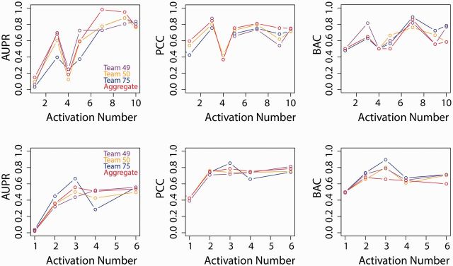
Team scores for the various metrics as a function of the number of stimuli for which a given protein is active (top) and the number of active proteins for a given stimulus (bottom)

Because the split of the stimuli into a training and test set was performed by the challenge organizers after observing the phosphorylation and gene expression patterns, we have tested whether the particular split led to unusually low or high prediction performance. The method of Team 49 was applied on 25 random splits of the stimuli into training and test sets. The mean BAC over the 25 trials was 0.66 (SD = 0.06), whereas mean Pearson correlation was 0.68 (SD = 0.05). These values are very similar to those reported in Table 1, and hence, there was no evidence that the split of the stimuli that was used in the challenge was particularly favorable to the development of prediction models, and hence, with other splits the performance results would have been similar. However, when the phosphorylation status was set randomly to each stimulus in the training set, the mean BAC over the 25 trials was 0.55 (SD = 0.04), whereas mean Pearson correlation was 0.56 (SD = 0.05).

We have also determined the persistence of the predictor genes of Team 49’s method across the 25 trials in which training stimuli were randomly selected among all 52 involved in the challenge. The percentage of the trials in which a given predictor gene was selected of all instances when a model could be built (the protein was phosphorylated for three or more stimuli), are reported in Supplementary Table S2 for genes selected in >33% of the trials. A number of 6 of these 17 more reliable gene predictors were also found by two or more of the three teams during the challenge. As an example, for protein MK03, genes WISP1 and DIO3 were selected in > 50% of the trials, and both were among the predictors identified in the challenge by Team 49 (see Supplementary Table S1) with DIO3 gene being also found by Team 50, as shown in Table 2.

4 DISCUSSION

Animal models are often used in biomedical research for testing the effect of various stimuli (e.g. drugs) before considering them for testing in humans. The general assumption is that biological processes in animals (e.g. mice or rats) are similar to biological processes in humans under analogous conditions. However, few studies have addressed the limitation on which biological events observed in rodents can be translated to humans. For instance, gene expression level changes in murine and human models were not at all correlated in peripheral blood as a response to inflammatory injuries, such as burns, blunt force trauma, as well as to endotoxin in human patients and in mice (Seok et al., 2013). The Species Translation Challenge, comprising four sub-challenges, was developed to systematically assess translatability of protein phosphorylation and pathway activation in response to a range of stimuli. The aim of the first sub-challenge, the ‘intra-species protein phosphorylation prediction sub-challenge’, was to assess whether downstream (in time) gene expression data are sufficiently informative to infer protein phosphorylation status of some key signaling molecules, and provide a baseline performance expectation for the translation from rat to human.

Three teams ranked first in this challenge, based on the fact that their performance was not distinguishable by the prespecified ranking methodology (Table 1). The performance of these three teams was also significantly better than any one of the remaining teams, as determined using a rank stability analysis. The prediction performance results of these top ranked teams suggest that a snapshot of the transcriptomic activity in rat epithelial cells contains a moderate level of information regarding protein phosphorylation levels, with the average sensitivity and specificity being about 70%. Improved performance might be obtained if the gene expression data were collected at multiple time points following treatment, to capture important time-dependent effects, non-linearity and multi-node cooperation in gene–protein interactions.

In this article, we have described in detail the approaches of the three teams tied for first place in this sub-challenge. Each team used a different method to select predictor genes, namely, ranking genes by moderated t-test P-values between classes and choosing a handful of the top ones (Team 49), using MI between each gene and the outcome and performing dimensionality reduction via PCA (Team 50) and performing gene ranking by ridge regression (Team 75). A large variation in the number of predictor genes was observed for each given protein from one team to the next with the most parsimonious approach (Team 49) using on average less than four predictor genes. Moreover, the types of models used to make predictions based on the selected genes were also very different among teams. Team 49 used an LDA model. Team 50 used a voting procedure, which combined the predictions from a method based on MI with one based on an LDA model trained on principal components. Team 75 results were based on SVR with RBF kernels. However, an important aspect of the model development was common among the three teams, namely, that the optimal number of predictors used was automatically determined based on cross-validated model performance, even though the specific performance metrics used were different. This element was also in common among the best and third best teams in the IMPROVER Diagnostic Signature Challenge (Tarca et al., 2013a). Despite the very different prediction approaches and gene signatures, the performance results of these three teams were very similar. The main reasons for this were (i) a redundancy in the gene signatures of Teams 50 and 75 and (ii) strong correlations between predictor genes selected by different teams (as suggested by Figure 5). Although an analysis of the overlap of predictor genes found more common genes than expected by chance among the three teams, this analysis did not account for extra overlap that could have occurred simply by modeling the noise in the data, i.e. when the phosphorylation status of proteins were randomly assigned to the different training stimuli.

Another common aspect among the approaches described herein is the fact that they used only information from the training data to make inference on the phosphorylation status of the 16 proteins after treatment with stimuli in the test set. Alternative approaches could have relied at least in part on prior knowledge regarding the target genes of the 16 proteins under the study. The top three teams considered that an unbiased approach, in which all genes are treated as potential candidates for being informative of the phosphorylation status of a given protein would have a better chance to maximize prediction performance than relying on the literature evidence of potential gene targets for each protein. Moreover, these data-driven methodologies can be applied to proteins for which no potential targets are available.

A KEGG (Ogata et al., 1999) pathway enrichment analysis (Falcon and Gentleman, 2007) on the union of predictor genes from the three teams was done to determine whether biological pathways are activated for each of the phosphorylation proteins. We found that five proteins have at least one enriched pathway (false discovery rate of 10%). The results are presented in the Supplementary Table S3. This analysis found also that almost half of the predictive genes associated with FAK1 and PTN11 activity are related to metabolism pathways. This should not be surprising because metabolism is a fundamental process that the cell regulates in response to any stress. However, it suggests that genes related to metabolism may be the best predictors of phosphorylation activity. For PTN11, we also found activation of four gene sets, which are related to signaling in cancer (Bentires-Alj et al., 2004). Similarly, for MK14K11, two cancer-related pathways show some evidence of enrichment, although not significant after adjustment for multiple testing. This is consistent with the role of MK14K11 in cancer signaling and, in particular, P53 activation. For IKBa, we found that many enriched pathways are related either to metabolism or to the function of IKBa as a key regulator of the immune response nuclear factor kappa-light-chain-enhancer of activated B cells (NFkB) pathway. A limitation of this analysis is that the predictor genes of the most two parsimonious approaches, Teams 50 and 49, have limited or no contribution, respectively, to the pathway enrichment results, as the union of predictor genes for each protein is dominated by genes selected by Team 75.

In summary: The ‘intra-species protein phosphorylation prediction’ sub-challenge of the IMPROVER Species Translation Challenge was designed to identify the extent to which it is possible to predict upstream protein phosphorylation effects from a snapshot of downstream transcription activity. This crowdsourcing initiative identified three approaches, described in detail herein, that were ranked best among 21 participating teams. Two of these three approaches (Teams 50 and 49) were also applied successfully in the ‘inter-species protein phosphorylation prediction (SC2)’, and therefore, SC1 represented a case study for the different teams to tune their approaches for SC2. Moreover, comparing the performance of the same approach (e.g. Team 49) between SC1 and SC2, we could conclude that when using only gene expression data to predict protein phosphorylation, the inter-species prediction problem (SC2) was only slightly more difficult than the intra-species prediction (SC1) (BAC and Pearson were almost identical with AUPR being 0.09 units less in SC2 than in SC1 for Team 49). In addition to providing an estimate for the best performance to be expected in such an experimental design (about 70% BAC that was significantly better than expected by chance; see performance breakdown per protein in Supplementary Table S4), the results described here also provide informative gene signatures for the phosphorylation activity of 16 proteins in rat lung epithelial cells under various stimuli. The prediction performance did not depend on the particular choice of training stimuli (of the 52 used in the challenge), yet only few predictor genes were stable over different sets of training stimuli and gene selection methods.

REFERENCES

- Basak D, et al. Support vector regression. Neural Inf. Process. Lett. Rev. 2007;11:203–224. [Google Scholar]
- Bentires-Alj M, et al. Activating mutations of the noonan syndrome-associated SHP2/PTPN11 gene in human solid tumors and adult acute myelogenous leukemia. Cancer Res. 2004;64:8816–8820. doi: 10.1158/0008-5472.CAN-04-1923. [DOI] [PubMed] [Google Scholar]
- Chang CC, Lin CJ. LIBSVM: a library for support vector machines. ACM Trans. Intell. Syst. Technol. 2011;2:27. [Google Scholar]
- Cortes C, Vapnik V. Support-vector networks. Mach. Learn. 1995;20:273–297. [Google Scholar]
- Cover TM, Thomas JA. Elements of Information Theory. Hoboken, New Jersey, USA: John Wiley & Sons; 2012. [Google Scholar]
- Falcon S, Gentleman R. Using GOstats to test gene lists for GO term association. Bioinformatics. 2007;23:257–258. doi: 10.1093/bioinformatics/btl567. [DOI] [PubMed] [Google Scholar]
- Gentleman RC, et al. Bioconductor: open software development for computational biology and bioinformatics. Genome Biol. 2004;5:R80. doi: 10.1186/gb-2004-5-10-r80. [DOI] [PMC free article] [PubMed] [Google Scholar]
- Hastie T, et al. The Elements of Statistical Learning. Vol. 2. New York, NY, USA: Springer; 2009. [Google Scholar]
- Ogata H, et al. KEGG: kyoto encyclopedia of genes and genomes. Nucleic Acids Res. 1999;27:29–34. doi: 10.1093/nar/27.1.29. [DOI] [PMC free article] [PubMed] [Google Scholar]
- Rhrissorrakrai K, et al. Understanding the limits of animal models as predictors of human biology: lessons learned from the sbv IMPROVER Species Translation Challenge. Bioinformatics. 2015;31:471–483. doi: 10.1093/bioinformatics/btu611. [DOI] [PMC free article] [PubMed] [Google Scholar]
- Seok J, et al. Genomic responses in mouse models poorly mimic human inflammatory diseases. Proc. Natl Acad. Sci. USA. 2013;110:3507–3512. doi: 10.1073/pnas.1222878110. [DOI] [PMC free article] [PubMed] [Google Scholar]
- Shannon CE. A mathematical theory of communication. ACM SIGMOBILE Mob. Comput. Commun. Rev. 2001;5:3–55. [Google Scholar]
- Tarca AL, et al. Machine learning and its applications to biology. PLoS Computat. Biol. 2007;3:e116. doi: 10.1371/journal.pcbi.0030116. [DOI] [PMC free article] [PubMed] [Google Scholar]
- Tarca AL, et al. Strengths and limitations of microarray-based phenotype prediction: lessons learned from the improver diagnostic signature challenge. Bioinformatics. 2013a;29:2892–2899. doi: 10.1093/bioinformatics/btt492. [DOI] [PMC free article] [PubMed] [Google Scholar]
- Tarca AL, et al. Methodological approach from the best overall team in the sbv improver diagnostic signature challenge. Syst. Biomed. 2013b;1:24–34. [Google Scholar]
- Vapnik V. The Nature of Statistical Learning Theory. Springer-Verlag, New York: Springer; 2000. [Google Scholar]
Associated Data
This section collects any data citations, data availability statements, or supplementary materials included in this article.