DIME: A Novel Framework for De Novo Metagenomic Sequence Assembly

Abstract

The recently developed next generation sequencing platforms not only decrease the cost for metagenomics data analysis, but also greatly enlarge the size of metagenomic sequence datasets. A common bottleneck of available assemblers is that the trade-off between the noise of the resulting contigs and the gain in sequence length for better annotation has not been attended enough for large-scale sequencing projects, especially for the datasets with low coverage and a large number of nonoverlapping contigs. To address this limitation and promote both accuracy and efficiency, we develop a novel metagenomic sequence assembly framework, DIME, by taking the DIvide, conquer, and MErge strategies. In addition, we give two MapReduce implementations of DIME, DIME-cap3 and DIME-genovo, on Apache Hadoop platform. For a systematic comparison of the performance of the assembly tasks, we tested DIME and five other popular short read assembly programs, Cap3, Genovo, MetaVelvet, SOAPdenovo, and SPAdes on four synthetic and three real metagenomic sequence datasets with various reads from fifty thousand to a couple million in size. The experimental results demonstrate that our method not only partitions the sequence reads with an extremely high accuracy, but also reconstructs more bases, generates higher quality assembled consensus, and yields higher assembly scores, including corrected N50 and BLAST-score-per-base, than other tools with a nearly theoretical speed-up. Results indicate that DIME offers great improvement in assembly across a range of sequence abundances and thus is robust to decreasing coverage.

1. Background

Metagenomics is the study of all micro-organisms coexistent in an environmental area, including environmental genomics, ecogenomics, or community genomics. In the past, microbial genomic studies usually focused on one single individual bacterial strain that is suitable to be separately cultivated (Wu et al., 2007). However, there are limitations when it comes to separately culturing individual stain. This is because, first, an isolate bacterial strain functions differently in isolation compared to when it works in communities. Due to experimental limitations, most of the microbes could not be isolated in laboratory conditions and, in fact, all micro-organisms in a habitat have various functional effects on one another and their hosts, such as the human gut (Gill et al., 2006) and larger ecosystems (Venter et al., 2004). Research (Qin, 2009; Khachatryan et al., 2008; Lin et al, 2009) has shown the strong association between common diseases and the diversity of microbes in humans, like inflammatory bowel disease and gastrointestinal disturbance. For this reason, studying how these micro-organisms function is crucial for any project involving curing these diseases. Population sequencing is an essential tool for recovering the genomic sequences in a genetically diverse environmental sample, which is known as metagenomics and also known as environmental genomics or community genomics. These studies are fundamental for identifying and discovering novel genes; studying ecosystems by utilizing other bioinformatics tools, like multiple sequence alignment services (Nguyen, 2012); and hence advancing our systemic understanding of biological processes and communities.

With high-throughput next generation sequencing (NGS) technology, like the 454 technology (Turnbaugh, 2009), solutions for metagenomics analysis become possible. Using automatic tools such as MG-RAST (Meyer et al., 2008), biologists can analyze the reads in the environmental sample by aligning them against known genomes, protein families, and functional groups in order to grossly obtain the structure of taxonomy of species and discover genes. The NSG platforms not only dramatically increase the size of sequencing datasets in large metagenomic projects (He et al., 2013), but also shorten the average length of reads with high coverage on the genomes. As demonstrated by the study of Meyer et al. (2009), assembled sequences help extract more information from the reads and leads to the discovery of more genes and better functional annotation than using short and noisy individual reads. Current methods for metagenomic sequencing assembly are deficient in generating high-quality assembled contigs and handling the large scale of data, particularly for terascale metagenomics projects. For instance, 454 Roche GS Titanium system could collect 200 Mbp to 300 Mbp data within 5 hrs. Typically, existing popular assembly tools lack the ability to achieve a good trade-off between the noise of the resulting contigs and the gain in sequence length for better annotation in large-scale sequencing projects (Pignatelli and Moya, 2011). As far as we know, there are a few de novo assemblers aiming at metagenomics (Pignatelli and Moya, 2011), including MetaVelet (Namiki et al., 2011), Genovo (Laserson et al., 2010), and MetaIDBA (Peng et al., 2011). By analyzing our experimental results, we can find that some methods, like Genovo, assemble the sequences too long to obtain correct matching on the reference genome, while for other methods, like MetaVelvet and SOAPdenovo (Luo et al., 2012), reported consensus sequences are too short for further analysis.

In order to address the aforementioned problems, we present a novel framework based on DIvide, conquer, and MErge strategies (DIME) for de novo metagenomic assembly. The four phases framework of DIME are summarized as follows:

• • Weight-edge construction (WEC). A weight graph is built to capture the chances that two reads share a common area sequenced from the same section on the sequence. We first scan all reads to count the number of l-mers shared between them by transforming a read into a string of l-mer. We then select pairs of reads to calculate their similarity scores based on the Smith-Waterman algorithm (Smith and Waterman, 1981), if they share at least β common l-mers.

• • Clustering. A graph partition algorithm is applied to the weight graph to split the set of reads into disjoint subsets with nearly balanced sizes. The basis for clustering is that gaps often remain after initial contig construction. By separating reads into groups, reads with high similarity to a certain group will not disrupt the assembly on that group.

• • Local-assembling. Traditional overlap-layout-consensus (OLC) assembly tools, including Cap3 and Genovo, are used to run locally for each reads cluster to generate a set of candidate contigs.

• • Merging. A global merging procedure is applied to combine the candidate contigs, correct chimeric reads, and refine consensus sequences based on the generative probabilistic model.

The four phases framework can be easily deployed on cloud platform, and we give two implementations on a Hadoop cluster. One of the advantages of cloud technologies is that a large distributed infrastructure can be readily accessed by nondistributed computing experts since the whole execution environment and experimental conditions can be easily customized. In addition, as the infrastructure is rented on a pay-per-use basis, immediate access and release to the required resources become possible without planning beforehand (Guo et al., 2013). As far as we know, many other bioinformatics tools have been implemented in Hadoop platform, including Crossbow (Langmead et al., 2009) and Contrail (Schatz et al., 2010). Crossbow is for searching SNPs. Contrail aims to assemble Illumina datasets, and it relies on the graph-theoretic framework of de Bruijn graphs. The reported contigs by Contrail only achieved similar size and quality to those generated by Velvet (Namiki et al., 2011), so we drop Contrail in the experiment and select other two de Bruijn graph–based methods, MetaVelvet (Namiki et al., 2011) and SOAPdenovo (Luo et al., 2012), which are claimed to be better than Velvet.

For a systematic evaluation of the performance of DIME, we compare DIME to five other popular short read assembly programs: Cap3 (Huang and Madan, 1999), Genovo (Laserson et al., 2010), MetaVelvet (Namiki et al., 2011), SOAPdenovo (Luo et al., 2012), and SPAdes (Nurk et al., 2013), on four synthetic and three real metagenomic sequence datasets with various reads, from fifty thousand to a couple of million in size. A bunch of commonly used metrics (Salzberg et al., 2012), including N50, corrected N50, unaligned reference bases, and unaligned assembly bases, demonstrate that DIME not only gives a high accuracy partition of the sequence reads, but also reconstructs more bases and yields a better quality assembly than other tools with nearly theoretical speed-up on a Hadoop cluster. In addition, the four phases framework of DIME is very flexible to support other next generation sequencing platforms, like Illumina, with some minor modifications, which are also a future direction for DIME. Therefore, we believe DIME is a promising framework for large metagenomic projects with diminishing coverage.

2. Materials and Methods

In the de novo assembly of environmental samples, the number, length, and content of these sequences are uncertain. With the observation that gaps often remain after initial contig construction, isolated overlapping DNA sequences can be clustered and assembled separately. The overall sequenced sample can be considered as a weight undirected graph, where a vertex represents a single fragment, and an edge represents the chance that two reads share an area from the same section on the genome. A balanced graph partition algorithm can be effectively applied to the graph, and the reads set can be grouped into disjoint sets. Existing assembler then will be executed in parallel for the separated reads set. Due to the similarity of genomes between closed species in environmental samples, erroneously grouped DNA fragments are inevitable. In order to cope with the erroneous clustering and further improve the assembly quality, another phase with generative probabilistic model is formulated to represent the sequencing procedure that DNA reads are obtained as noise copies of contiguous parts of the contigs. The novel assembly framework with four phases is proposed to seek the best trade-off between the noise of contigs and the gain in length of consensus sequence for a better annotation. Furthermore, the novel assembly framework can be well cast into the popular MapReduce programming model and deployed on commercial cloud platform. In the following paragraphs, we elaborate our novel metagenomic sequencing assembly framework in four phases with the Map-Reduce task designs. Figure 1 outlines the four phases of our method.

FIG. 1.

The pipeline of DIME. DIME is divided into four major phases: weight-edge construction, clustering, parallel-genovo, and merging.

2.1. Phase I: Weight-edge construction (WEC)

2.1.1. Notations

The entire read set is denoted as R, and we assume that there are n reads. Let r_i be the i-th read (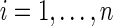), and |r_i| be the length of the read i. Given a fix length η of l-mer, read i can be represented as a string of (|r_i|− η + 1) l-mers. Let L denote the set of all different l-mers, and l_j be the j-th l-mer in the alphabet order. Giving a specific l-mer l_j, we define a set H_j consisting of the reads, which have l_j in their strings. Given two reads r_a and r_b, the chance that they can be concatenated is denoted as CHC(r_a,r_b).

2.1.2. WEC

The purpose of weight-edge construction (WEC) is to build a weighted graph where a vertex represents a read and the weight on an edge represents the measure of the chance that two linked reads by this edge share an area that is sequenced from the same section on the genome. Two issues are raised from this phase:

• 1. It is computationally unacceptable to exhaustively calculate all weights, if we have hundreds of thousands of reads (the total number of weights is ). Moreover, if two reads differ greatly from each other, which is usually the case in the sequencing sample, the existence of the edge itself is unnecessary.

• 2. How to define the weight function to capture the chance CHC(r_a,r_b) given two reads r_a and r_b.

In order to cope with the two concerns, we design two procedures: (1) scanning and (2) aligning, which are adapted from two methods, ZEBRA algorithm (Grillo et al., 1996) and Smith-Waterman (SW) dynamic programming algorithm (Smith and Waterman, 1981), respectively. ZEBRA uses a fast scanning rule to skip nonmatch reads, and SW is a classical local alignment algorithm. The details of the sequential WEC is as follows:

• 1. We first transform all reads into strings comprising only l-mers.

• 2. For each l-mer l_j, we construct the set H_j, which comprises the reads that have l_j in their strings. We then get a table with two columns. The first column is for L (the set of all l-mers), and the second column is for the set H_j. Each row represents the pair of l_j and its set H_j.

• 3. We split the set H into two disjoint parts, H′ and H′′. If the cardinality of H_j is less than a predefined threshold maxH, we put H_j into H′, otherwise it goes to H′′. The reasons that we need maxH are twofold: (1) l-mers coming from the repeated regions on the genome are not so important as the rest of the l-mers, because a unique l-mer indicates a high probability that reads with the l-mer are from the same sequence, while the former does not have this attribute. (2) In our MapReduce implementation, we need to enumerate all the subsets of H_j with only two members and send them back and forth among computing nodes. If |H_j| is large, the communication cost is too high.

• 4. For the reads in H_j ∈ H′, we generate all the pair combinations of reads, and repeat for every j. We then count the frequency for each unique pair as fre_ra,rb given reads r_a, r_b.

• 5. We need to filter out pairs of reads that are less possible to be adjacent on the sequence. If fre_ra,rb ≥ β, we put the pair (r_a, r_b) into a candidate list. If fre_ra,rb < β, we search (r_a, r_b) in H_j ∈ H′′, and increment fre_ra,rb each time, when we find a pair. We add the pair into the candidate list if it is not less than the threshold.

• 6. For the pairs in the candidate list, we use SW to get the local alignment and obtain the CHC by the following formula:

  where the s_h, s_m, s_in, s_d are the unit scores for the hit, miss, insert, and delete bases, and the n_h, n_m, n_in, n_d are the counts of the corresponding base pairs, respectively.

• 7. We connect two vertexes a and b in the weighted graph if we obtain a value of CHC(r_a, r_b), which is the weight on the edge.

More details of the algorithm of WEC can be found in the Supplementary Material (available online at www.liebertpub.com/cmb). In the above steps, two parameters maxH and β are applied. maxH aims to reduce the computational burden and save communication cost because of the repeat region on the genome. We do not suffer information loss since |H_j| ≥ maxH goes to H′′, and the rest pairs of reads with frequencies less than β will be evaluated if those pairs show up in H. In our experiments, we set maxH to twenty times the expected value of |H_j|. For example, if we fix η to eight letters, and there are 1,000,000 reads, then the expected frequency of reads having a certain l-mer is , so we set maxH to 320. The setting of β is related to the error rate of the sequencing platform. In Margulies et al. (2005), an error rate of about 3% is reported. We treat a pair of reads as candidates for alignment, if they overlap at least 25 bp. Based on the error rate, it is expected that there are 10 l-mers sharing between them, if we fix η to 8 bp. We will set β to a slightly smaller value than 10 instead. From the experimental results in section 3.4, this setting for β can achieve acceptable clustering accuracy. The MapReduce implementation of WEC can be found in the Supplementary Material.

2.2. Phase II: Clustering

In clustering, we partition the set of reads into disjoint subsets with balanced size, and one property of each subset by partition is that the average weight of reads in the same subset is larger than the average weight of reads from different subsets. The weights are from local alignment in phase I. The details of algorithm 2 for clustering can be found in the Supplementary Material. Specifically, we design clustering based on the following considerations:

• 1. We first predefine a number of result cluster N, and set the maximum cardinality of a cluster to (where α ≥ 1 is a scale factor.)

• 2. Since the graph generated in WEC may have multiple connected components, we set the target to the connected component instead of the whole graph. For each connected component, if the cardinality of vertex set is less than or equal to , we keep it unchanged; otherwise, we use a k-way graph partitioning algorithm, Kmeits (Karypis and Kumar, 1999), to partition the component until all the partitions have the cardinality no larger than . Because the graph partitioning problem is NP-complete, we are not going to redesign a new algorithm to deal with it. We adopt Kmetis (Karypis and Kumar, 1999) to handle this tough job. More details of Kmeits can be found in the Supplementary Material.

2.3. Phase III: Local-assembling

Through the above two phases, N sets with a limited number of reads are generated, and they can be treated as separate and independent sequence assembly jobs. In the local-assembling (LA), we modify the input and output parts of existing assembly tools, like Cap3 and Genovo, and wrap them up in the Hadoop platform, which can automatically regulate the workload balance among the computing nodes. Note that, in DIME, only overlap-layout-consensus (OLC) methods are applied. The OLC methods use an overlap graph where nodes represent the reads and edges represent overlaps between reads. The overlaps are precomputed by a series of pairwise sequence read alignments. A reason that we select OLC methods is that for the refinement of candidate contigs from phase III, we need the count information of every base on the candidate contigs (Fig. 2) to build a generative probabilistic model, and further merge and promote the quality of assembly. More details of Cap3 and Genovo are described in the following paragraphs.

FIG. 2.

Count of each deoxyribonucleic acid for one base on the contig. Reads coverage information from local assembler in phase 3.

2.3.1. Local-cap3

The Cap3 assembler proposes a method to resolve assembly problems in the form of the third generation of CAP sequence assembler. It clips 5′ and 3′ poor regions of reads, uses forward-reverse constraints to correct errors in construction of contigs, and generates consensus sequence for contigs. Among these features, the most outstanding is the algorithm for making use of constraints to correct assembly errors. The algorithm performs a correction only if the correction is supported by a sufficient number of constraints. The random distribution of subclones indicates that errors in constraints are also randomly distributed. Therefore, it is unlikely that a sufficient number of wrong constraints all consistently support a correction to the same region. If quality values are not available, Cap3 is the better choice, because Cap3 is able to make full use of redundant coverage in the construction of consensus sequences. Like the other OLC methods, Cap3 consumes much more time as the size of the datasets increases. For instance, a typical sequencing reads set from the 454 platform that reaches up to millions of reads will require around 40 hours to get the contigs.

2.3.2. Local-genovo

Our algorithm for local-genovo derives from the metagenomes de novo assembly approach, Genovo (Laserson et al., 2010). The reason we choose Genovo is that it can reconstruct more bases and produce an assembly with better quality, especially for the low-abundance dataset compared to other methods. Genovo is an instance of iterated conditional modes (ICM) algorithm, which sequentially performs a random walk on states corresponding to different assemblies for maximizing local conditional probabilities. The drawback of Genovo is the computation time. Take a middle-size metagenomic dataset, for example, which have 220k reads with 400 bp as average length; Genovo consumes more than 37 hr on a typical desktop computer in our experiments. The local-genovo is modified to run on the Hadoop platform and to produce a set of contigs with the count information in the structure as shown in Figure 2. The count information are from those reads covering the current base. The frequency is also employed to compute the global merging in phase IV.

2.4. Phase IV: Merging

The merging phase is designed to further merge and refine the candidate contigs for creating high quality of assembly. In this phase, three general questions are addressed:

• 1. How to decide whether two contigs should be merged together.

• 2. How to identify and correct indel bases on overlap of two contigs when they're merged.

• 3. How to remove the chimeric reads (Lasken & Stockwell, 2007), that is, a prefix or a suffix matching distant locations in the genome.

2.4.1. Generative probabilistic model

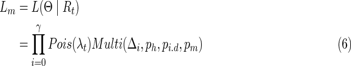
For the first question, we present a generative probabilistic model to describe the process of next generation sequencing. When a DNA fragment is sequenced from the genome, the sequencing model is Θ = (λ, p_h, p_i.d, p_m), with λ representing the expectation of how many reads will cover a single base and p_h, p_i.d, p_m denoting the probabilities for base hit, insertion and deletion, and mismatch, respectively. We assume that the number of short sequencing reads, X, covering a single base on the genome, follows Poisson distribution (Lander and Waterman, 1988) with parameter λ:

In the generative probabilistic model, we estimate the parameter λ as the average count of reads covering a base given the assembled contig from phase III. By giving a consensus sequence with reads covering it, we estimate the p_h, p_i.d, p_m as the average hits, indels, and mismatches per base; for example, considering a consensus sequence with 10 pb and 9 hits from 10 reads per base, then we set for that assembled part.

For any base with symbol B () on the contig or consensus, let δ_h denote the count of reads covering the same position by the same symbol as B, let δ_i.d denote the count of reads skipping this base, and let δ_m denote the count of reads covering the base but with another symbol different from B. We further assume that the vector 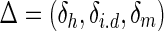follows a multinomial distribution with parameters k and P = (p_h, p_i,d, p_m), which are

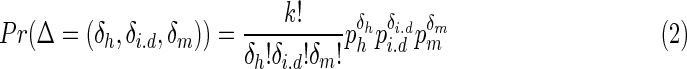Given a set of aligned reads, R, the likelihood generating the candidate contig by our model within the interval [a, b) is

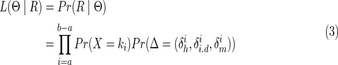Taking Equations 1 and 2 to Equation 3, we can get the following likelihood

Suppose we get an alignment t of two contigs t_u,t_v, which will be discussed in the next section, two likelihoods can be calculated. The first is before merging, L_b, and the second is after merging, L_m, assuming that the range of alignment covering on T_i is [a, b), and the corresponding range on T_j is [c, d) with a length γ on the alignment with all the inserted and deleted bases. L_b and L_m are defined as follows:

Based on Equations 5 and 6, we merge the two candidate contigs if L_b < L_m, otherwise we keep them unchanged.

2.4.2. Consensus sequence and chimeric reads

For the second question, we treat the process of sequencing as a multinomial distribution with three parameters p_h, p_i.d, p_m for the probabilities of hit, insertion and deletion, and mismatch per base. Since there are four letters for one base, we set the base on consensus to one letter each time and compute the probability using Equation 2. Note that if there is a deletion happening on the consensus, we insert a special letter “−” as empty. Therefore, we can get five probabilities for five hypotheses, and the letter with the highest probability will be the final symbol on the consensus.

For the third question about removing the chimeric reads, we align two ends of contigs in four different states: both with end reads that are placed on the ends of the contigs, only the first contig with the end read, only the second contig with the end read, and both without end reads. Thus, only the state with L_b < L_m can be further merged for two candidate contigs.

2.4.3. Mapreduce implementation for merging

In phase IV, we first use three MapReduce tasks as shown in phase I to determine a candidate list, which consists of contig pairs. The difference is that we use contigs instead of reads. A merging process is executed sequentially to calculate the likelihoods based on our generative probabilistic model, and refine each base on the consensus using the multinomial distribution. The procedure of merging is given in Algorithm 3. More details about Algorithm 3 can be found in the Supplementary Material.

3. Results

We compared the performances of two cloud implementations of DIME (DIME-cap3 and DIME-genovo) to four popular assembly tools—Cap3 (Huang and Madan, 1999), Genovo (Laserson et al., 2010), MetaVelvet (Namiki et al., 2011), SOAPdenovo (Luo et al., 2012)—and SPAdes (Nurk et al., 2013) on both simulated and real metagenomic datasets from the 454 platform. Following the measurement employed in Salzberg et al. (2012), seven metrics were used to assess the quality of reported contigs: assembly size, number of contigs (Num), longest length of contigs (LLC), N50, CorrN50, unaligned references bases (URB), and unaligned assembly bases (UAB) for simulated datasets. For real dataset, in addition to LLC and N50, we used another metric, BLAST-score-per-base (Bspb), to evaluate the performance. We also illustrated the scalability of our novel assembly framework in four aspects, including the running time comparison of Cap3, Genovo, DIME-cap3, and DIME-genovo; running time analysis for four phases of DIME; memory usage; and the speed-up of DIME. Note that MetaVelvet and Genovo are specially designed for metagemomic assembly. MetaVelvet, SOAPdenovo, and SPAdes are specialized for Illumina Genome-Analyzer platform, but they also support 454 reads. According to the suggestions of a recent article (Treangen et al., 2013; Nurk et al., 2013), SOAPdenovo and SPAdes can do very well for metagenomic datasets. We dropped Newbler, the 454 Life Science de novo assembler, and IDBA-UD, because Genovo and SPAdes claimed to gain higher quality results compared to them (Laserson et al., 2010; Nurk et al., 2013). More details on the settings of parameters for these four tools can be found in the Supplementary Material.

3.1. Evaluation metrics

As done in previous studies (Laserson et al., 2010; Qin, 2009), we evaluated only contigs longer than 500 bp unless otherwise stated. The N50 value x is the size of the smallest contig such that 50% of the genome is covered by contigs of length ≥ x. The CorrN50 value is the N50 for the corrected contigs. Following the procedure in Salzberg et al. (2012), we aligned the reported contigs to the reference genomes by BLAST (Altschul et al., 1990), and corrected the contigs by breaking them at every misjoin and at every indel longer than five bases. URB are the reference sequences covered by simulated reads that do not align to any contig. UAB are contig sequences that do not align to the reference genome (Salzberg et al., 2012). Therefore, for URB and UAB, the lower the value, the better the quality of assembly. Note that only one aligned interval with the highest bit score (similarity ≥ 95%) can be counted as a valid matching even if one contig has multiple matchings on the references, or the reference has more than one contig aligning to it. Assembly size, URB, and UAB are expressed as a percentage of the reference sequence size or assembled contigs size. We declared in the introduction that a common bottleneck of available tools is hard to seek a good trade-off between the noise of the resulting contigs and the gain in sequence length for better annotation. So we define another metric, F-accuracy, which can be interpreted as a weighted average of URB and UAB:

And the higher value of F-accuracy means the better coverage on both reference sequences and reported contigs.

For the real metagenomic sequencing datasets, since we do not have the actual list of genomes, corrN50, MPR, URB, and UAB are unavailable. In this case, we adopted the same indicator in Laserson et al. (2010), Blast-score-per-base (Bspb), to estimate the relationship between the quality and the number of sequence bases that the contigs cover. For Bspb, we used the GenBank's online tool to BLAST the reported contigs with default parameters, except for allowing 1000 hits. We then collected the BLAST hits to compile a pool of genomes that best represents the consensus of the dataset. We threw away the BLAST hits if the genome was not in the pool. The quality of the remaining BLAST hits was accessed by Bspb, which was calculated as the BLAST alignment score divided by the length of the aligned interval. We were then able to show the quantity vs. the quality of the pool bases covered by the result contigs by plotting a curve with varied align threshold of Bspb. If a contig had more than one BLAST hit on the same area of the genome, we counted it only once and used the highest Bspb value for those bases. More details about Bspb can be found in Laserson et al. (2010).

3.2. Experimental setting

We deployed our cloud-based de novo assembler on a 10-node cluster. Each node came with 16 GB main memory and quad-core Opteron(tm) processor 2376 under 2.3 Ghz. The cluster shared a 625 GB secondary storage that was under the control of HDFS. The typical Hadoop configurations were left without any changes, including the default 64 MB block size, 3 HDFS replication factor, and one master node for controlling. For the parameters used by DIME, we fixed l-mer length η = 12 and threshold of frequency β = 7, and assigned the number of clusters N = 30 for simulated and real datasets, except for the E. coli and Tilapia1 datasets at N = 10.

3.3. Data simulation

We took the existing program, MetaSim (Richter et al. 2008), to artificially construct four metagenome sequence read datasets with different complexity. According to the simulation conducted in Pignatelli and Moya (2011), we selected 112 different species from the NCBI bacteria genome library as the genome pool. The first dataset, named LC, had only two dominant organisms, which are strongly taxonomically related. The second dataset, named MC, had a few dominant organisms. The third dataset, HC, did not have a dominant organism; that is, all the species had equal weight to obtain a similar coverage rate. Since we aimed for a large metagenomic sequencing project using 454 platform, we resampled the HC dataset with the coverage of each genome 10 times higher than in the original dataset and named it the HCh dataset. The statistic summary of the four datasets are shown in Table 1. The individual composition of each dataset and the error profile of MetaSim are presented in the Supplementary Material.

Table 1.

Summary of the Simulated Datasets Used in This Study

Dataset	Number of species	Number of base pairs (Mb)	Number of reads
LC	112	89.5	220,288
MC	112	92.8	220,288
HC	112	91.2	220,288
HCh	112	1,077.2	2,202,880

LC, dataset with low complexity of organisms; MC, dataset with medium complexity of organisms; HC, dataset with high complexity of organisms; HCh, dataset created by resampling the HC dataset with the coverage of each genome ten times higher than in the original dataset.

3.4. Clustering experiment on simulated datasets

The general purpose of de novo sequence assembly is to recover consensus correctly. In DIME, the clustering process is one of the most important parts to achieve high quality assembly. So we defined a metric, clustering accuracy, to evaluate its performance. For the simulated datasets, each sequenced read came with its position on the original DNA sequences. If two reads share at least κ bases on the same genome and the same area, we consider them in the same ground-truth contig. In reality, assemblers can not align two reads together with insufficient overlap, so we set κ into three levels, 20, 30, and 40 bases. If most of the reads from the ground-truth contig t were grouped in cluster c, we then assigned t to c, and the reads sharing between the cluster and the contig, R_c ∩ R_t, was denoted as R_t′. The clustering accuracy is defined as follows

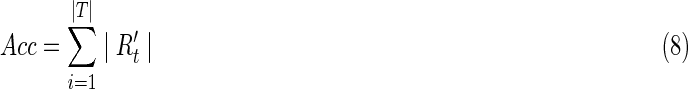Based on this definition, we used WEC and clustering to partition the read set into 5, 10, 20, 30, and 60 groups. The performance of clustering is shown in Table 2. In the worst case scenario that the read set is split into 60 groups for the LC dataset, the accuracy of DIME can still reach up to 94%. From the perspective of clustering accuracy, WEC and clustering procedures can highly recover the memberships of reads in terms of rough partition. In the following experiments, we clustered the reads set into 30 groups unless otherwise stated.

Table 2.

Clustering Accuracy on Simulated Datasets

		Length of minimum overlap2
Dataset	# Clusters1	20	30	40
LC	5	97.4%	98.2%	98.8%
	10	96.2%	97.2%	97.9%
	20	95.7%	96.7%	97.8%
	30	95.3%	96.4%	97.2%
	60	94.6%	95.8%	96.6%
MC	5	98.7%	98.9%	99.2%
	10	98.3%	98.6%	99.0%
	20	97.4%	97.7%	98.1%
	30	97.3%	97.6%	98.0%
	60	97.3%	97.6%	98.0%
HC	5	100.0%	100.0%	100.0%
	10	100.0%	100.0%	100.0%
	20	99.9%	100.0%	100.0%
	30	99.9%	100.0%	100.0%
	60	99.9%	100.0%	100.0%
HCh	5	99.0%	99.4%	99.6%
	10	98.9%	99.3%	99.5%
	20	98.6%	99.1%	99.4%
	30	98.5%	99.0%	99.4%
	60	98.0%	98.7%	99.1%

¹We manually set the output number of clusters to 5, 10, 20, 30, and 60.

²If most of reads from the ground-truth contig t were grouped in cluster c, we then assigned t to c, and the reads sharing between the cluster and the contig, R_c ∩ R_t, was denoted as . The clustering accuracy is defined as follows:

LC, dataset with low complexity of organisms; MC, dataset with medium complexity of organisms; HC, dataset with high complexity of organisms; HCh, dataset created by resampling the HC dataset with the coverage of each genome 10 times higher than in the original dataset.

3.5. Experiment on a single sequence dataset

Before the evaluation of the performances on metagenomic datasets, we benchmarked DIME on a single sequence dataset, E. coli, whose reference strand can be accessed from the NCBI short read archive. This dataset was sequenced by the 454 Titanium, and the total length of the genome of E. coli was 4.6 Mb, which contained around 110 k reads with an average length of 351 bp. In our experiment, we clustered the E. coli dataset into 10 groups since its size was relatively small. For URB and UAB, it is worth it to note that only one matching interval with the highest bit score (similarity ≥ 95%) can be counted as a valid matching if one contig has multiple alignments on the reference. As shown in Table 3, DIME-cap3 and DIME-genovo outperformed Cap3, Genovo, and SPAdes on URB and UAB, although the last two produced higher N50 or corrected N50. Higher values of URB and UAB strongly means more generated contigs are mistakenly constructed. Since the dataset and the genome of E. coli is small, our methods gained a slightly lower N50 and corrected N50 value by comparing to Cap3 and Genovo. However, DIME, Cap3, and Genovo gained higher value on both by comparing to MetaVelvet and SOAPdenovo, which means that de Bruijn graph–based methods may be not quite suitable to handle datasets by 454 platform.

Table 3.

Comparing the Methods on a Single Sequencing Task

	E. coli
Assembler	Assembly size (%)	Num1	LLC2(bp)	N501 (bp)	CorrN502(bp)	URB4(%)	UAB5(%)	F-accuracy3
DIME-cap3	105.7	822	43,534	9,731	8,600	19.9	25.4	0.77
DIME-genovo	101.0	408	111,514	24,546	12,514	33.4	35.8	0.66
Cap3	107.3	609	49,632	14,291	9,508	24.2	28.1	0.74
Genovo	105.5	90	203,303	95,468	24,009	58.7	59.2	0.42
MetaVelvet	95.6	1,452	20,708	4,553	4,065	18.6	14.8	0.83
SOAPdenovo	99.2	2,536	8,979	2,399	2,282	16.6	16.1	0.84
SPAdes	101.0	112	279,680	93,032	26,067	57.9	58.3	0.42

Only contigs of length ≥500 contributed to the statistics.

¹N50: the largest value y such that at least 50% of the genome is covered by contigs of length y.

²CorrN50: The CorrN50 value is the N50 for the corrected contigs. We aligned the reported contigs to the reference genomes by BLAST and corrected the contigs by breaking them at every misjoin and at every indel longer than 5 bases.

³F-accuracy: interpreted as a weighted average of URB and UAB, 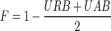. The higher F-accuracy, the better quality of results.

Num, number of contigs generated by assemblers; LLC, longest length of contigs; URB: unaligned reference bases; UAB, unaligned assembly bases.

3.6. Experiments on multispecies simulated datasets

We also tested DIME and five other tools on four simulation datasets to assess the performance. The summary of the statistics of reported contigs are listed in Table 4. An overview of the results indicates that DIME-genovo gained relatively higher corrected N50 on most cases except for the dataset MC. When the dataset became larger, de Bruijn graph–based methods, MetaVelvet and SOAPdenovo, did not perform as well as the overlap-layout-consensus methods. DIME and cap3 all obtained more than 700 on corrected N50, while MetaVelvet and SOAPdenovo stayed around 640. Another clear conclusion is that DIME recovered more bases than the other five tools. Although we set only one alignment to be counted when aligning to the reference to calculate unaligned reference bases (URB), DIME can still recover more than 90% of the reference for the dataset LC and more than 80% for the dataset HCh. In this respect, MetaVelvet, SOAPdenovo, and SPAdes only reported limited contigs that can be annotated on the reference sequence, although SPAdes did significantly improve the qualities of assemblies. For example, SPAdes only lost around 30% of the reference genomes for LC and HCh; Metavelvet lost more than 80% of the reference genomes for all four datasets, and SOAPdenovo lost more than 70% for all four datasets. In order to take both URB and UAB into consideration, we defined the F-accuracy in section 3.1. A higher value of F-accuracy indicates a better trade-off between the noise of assembled contigs and a better annotation. Our methods were much better than any other four assemblers in terms of F-accuracy with at most 40% improvement.

Table 4.

Summary of the Assemblies of Four Simulated Datasets

	LC
Assembler	Assembly size (%)	Num	LLC (bp)	N50 (bp)	CorrN50 (bp)	URB (%)	UAB (%)	F-accuracy
DIME-cap3	95.6	18437	3795	721	720	26.8	23.4	0.75
DIME-genovo	127.9	19406	42360	810	809	9.5	29.2	0.81
Cap3	66.3	13568	2588	688	687	50.3	25.2	0.62
Genovo	1.32	20317	28455	810	805	11.1	32.3	0.78
MetaVelvet	12.2	2684	1810	658	656	88.7	7.6	0.52
SOAPdenovo	17.1	3620	1380	721	718	84.7	10.8	0.52
SPAdes	67.8	5093	3795	1014	918	38.5	9.3	0.76

	MC
DIME-cap3	58.6	12960	2290	671	669	46.1	8.0	0.73
DIME-genovo	150.0	30704	5451	725	718	20.7	47.4	0.66
Cap3	25.2	5665	2842	660	658	77.1	8.8	0.57
Genovo	157.7	32006	4211	728	717	24.6	52.2	0.62
MetaVelvet	17.2	3878	1356	664	662	84.4	9.3	0.53
SOAPdenovo	21.7	5375	1667	707	700	78.5	1.2	0.60
SPAdes	55.6	7484	5522	847	747	63.1	33.6	0.52

	HC
DIME-cap3	57.3	11336	2338	676	675	45.3	4.5	0.75
DIME-genovo	163.7	30742	4247	711	704	15.2	48.2	0.68
Cap3	24.5	4901	1716	669	667	77.3	7.7	0.57
Genovo	171.4	31847	4541	717	703	16.0	51.0	0.66
MetaVelvet	13.2	2684	1810	658	656	87.7	7.6	0.52
SOAPdenovo	29.7	5612	1312	709	706	73.6	11.4	0.57
SPAdes	45.9	5863	5425	898	805	68.8	32.1	0.49

	HCh
DIME-cap3	81.5	362658	5096	735	733	33.7	18.6	0.74
DIME-genovo	98.8	308472	36761	1052	1045	15.9	14.9	0.85
Cap3	5.0	22852	4169	718	717	95.6	11.1	0.47
Genovo	NA	NA	NA	NA	NA	NA	NA	NA
MetaVelvet	10.6	54678	2526	637	637	89.8	4.8	0.53
SOAPdenovo	26.1	137401	1603	635	634	76.7	11.2	0.56
SPAdes	75.5	142296	37059	1200	1103	33.9	12.4	0.77

Only contigs of length ≥500 contributed to the statistics.

The value in bold indicates that the assembler obtained the highest F-accuracy.

When restricting the comparisons between DIME, Cap3, and Genovo, we can have some other interesting findings. With the divide, conquer, and merge strategies provided by DIME, we have more bases recovered and generate contigs with less noise. For instance, URB and UAB of Cap3 for LC were 50.3% and 25.2%, respectively, while DIME-cap3 lowered the former to 26.8% and the latter to 23.4% for the same dataset, and it also achieved higher corrected N50. It is also the same scenario for Genovo, where DIME-genovo decreased the URB from 11.1% to 9.5% and reduced the UAB from 32.3% to 29.2%. Scrutinizing the results of HCh, we found that Cap3 only assembled 5% of reference genomes, but DIME-cap3 can obtain 66.3% of the reference sequence. One explanation is that Cap3 is not suitable to assemble large sequencing datasets. By examining the unaligned reads, we found that most of them, which can be aligned in our method, were treated as singlets by cap3. Another explanation is that our generative probabilistic model used in the global merging process can successfully identify two adjacent contigs and combine them together. In our experiments, Genovo used up all the memory for the dataset HCh on a computing node with 32 GB memory and was finally killed by the system.

3.7. Experiments on real metagenomic datasets

We also conducted comparisons on three datasets from real metagenomic projects with different sizes of read sets (Table 5). The first dataset, named Tilapia1 (SRR001069), is sampled from the gut contents of hybrid striped bass containing microbial and viral communities. The number of total reads in this sample is about 50k with 5.7 Mb base pairs. The second real dataset is from the hot springs containing microbial communities with the name NTS (Vos et al., 2012). NTS is sequenced from Los Alamos National Laboratory. The largest real dataset is the third one labeled SRR072232 from NCBI. SRR072232 comes from the HMP Mock Community staggered sample by 454 sequencing platform, which is one of the largest real metagenomic sequence datasets we can freely download thus far. Since we do not have the true reference genome, we use the total length of contigs (TL) instead of the percentage indicator for the assembly size.

Table 5.

Summary of the Simulated and Real Datasets Used in This Study

Dataset1	Number of base pairs (Mb)	Number of reads
Tilapia1	5.7	50,211
NTS	254.5	683,082
SRR072232	653.1	1,225,169

¹Tilapia1 (SRR001069) is sampled from the gut contents of hybrid striped bass containing microbial and viral communities. NTS is sequenced from Los Alamos National Laboratory. SRR072232 comes from HMP Mock Community staggered sample by 454 sequencing platform.

The statistical analysis of results for seven programs on three real metagenomic datasets are shown in Table 6. Similar to the results in the simulation datasets, DIME-cap3 and DIME-genovo yielded comparable assembly on the small dataset—that is, Tilapia1—but both of our methods aligned more reads in the contigs and gained longer sequence compared to MetaVelvet and SOAPdenovo. Since there were around 600k reads in NTS and 1,200k reads in SRR072232, Genovo failed again by taking too much memory. For N50, DIME won much higher value for three datasets as compared to MetaVelvet and SOAPdenovo.

Table 6.

Summary of the Assembly Statistics of the Real Datasets

	Tilapia1
Assembler	TL (kb)1	Num2	LLC (bp)3	N50 (bp)4
DIME-cap3	48.7	51	1,896	1,017
DIME-genovo	53.6	59	3,767	939
Cap3	51.7	56	2,856	1,032
Genovo	56.3	49	6,510	1,062
MetaVelvet	1.0	2	541	541
SOAPdenovo	1.5	2	941	941
SPAdes	50.0	32	6,455	2,168

	NTS
DIME-cap3	25,054.6	32,032	4,284	773
DIME-genovo	70,998.3	108,765	9,617	558
Cap3	12,250.7	16,859	2,399	731
Genovo	NA	NA	NA	NA
MetaVelvet	4,809.8	7,542	1,560	627
SOAPdenovo	801.2	1,438	1,014	553
SPAdes	31,973.0	1,070	11,531	2,929

	SRR072232
DIME-cap3	59,664.2	60,399	10,142	1,012
DIME-genovo	63,752.6	57,122	45,359	1,155
Cap3	34,434.7	31,726	8,293	1,112
Genovo	NA	NA	NA	NA
MetaVelvet	8,357.7	13,369	2,573	603
SOAPdenovo	36,167.5	53,190	3,024	648
SPAdes	18,252.6	5,883	210,238	7,700

TL, total length of contigs; Num, number of contigs. LLC, longest length of contigs. N50, the N50 value x is the size of the smallest contig such that 50% of the genome is covered by contigs of length ≥ x.

To obtain a comprehensive comparison on real datasets, we adopted the same evaluation metric utilized in Laserson et al. (2010), that is, BLAST-score-per-base (Bspb). We followed the same procedures in calculating Bspb, and also the nonsignificant BLAST hit whose E-value was less than 10⁻⁹ was ignored. The highest Bspb can reach up to 1.88 in our experiments. Based on Bspb, the BLAST profile can be plotted by moving the threshold of Bspb from low to high. As shown in Figure 3, it is obvious that our methods cover more base pairs than Cap3, Genovo, MetaVelvet, SOAPdenovo, and SPAdes, along with decreasing the align threshold for NTS and SRR072232. Similar to the results on simulated datasets, although SPAdes had higher values for LLC and N50, Bspb values of SPAdes were not as good as others. This is because lots of contigs were incorrectly assembled. For Tilapia1, all the methods cover similar bases at the same align threshold, except MetaVelvet, which had less base hits when the align threshold was low.

FIG. 3.

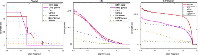
BLAST-score-per-base profiles for three real datasets. (a) BLAST profile on Tilapia1 and (b) BLAST profile on NTS and (c) BLAST profile on SRR072232 for our two methods (red and magenta solid lines), genovo (cyan dot line), cap3 (blue dot line), and metavelvet (green dot line).

3.8. Scalability

From a practical point of view, a key issue of metagnomic sequence assembly is computational efficiency. In this section, we evaluate the performances of DIME on Hadoop cloud platform with respect to its speed-up. To measure the speed-up, we first kept the size of datasets constant and increased the number of nodes (computing cores) in the cloud system, and then tried three different size settings considering the small, medium, and large datasets. The speed-up is defined by the following formula (Xu, et al., 2002):

where p is the number of nodes (computers), T₁ is the execution time on one node, and T_p is the execution time on p nodes. The ideal parallel method is expected to demonstrate a linear speed-up: a system with p computing nodes generates a speed-up of p. However, linear speed-up is only a theoretical predication, because the speed-up is always curved by either the inevitable failures of nodes, or communication cost, or both. In addition, the communication cost is increasing when we use more computing nodes in cluster. As shown in Figure 4, our two methods achieved nearly linear speed-up for two datasets, NTS and HCh, although two curves for the LC are slightly away from the theoretical linear line. Comparing with DIME-cap3 and DIME-Genovo, we can find that the performance of the latter is slightly better than the former. It is because Genovo tends to require more time to complete the assembly than Cap3 for the same reads set. By taking a look at the run-time of DIME on our 10-node cluster (Table 7), we found that WEC, local-assembling, and merging are the most time-consuming phases. And this exactly explains the theoretical speed-up achieved by DIME, since these three phases nearly perfectly fit into the MapReduce model.

FIG. 4.

Speed-up. Computing nodes are sampled from 1 to 10 with 1 as interval. The red, blue, and green curves show the speed-up of LC, NTS, and HCh. The black line is the linear speed-up.

Table 7.

Run Time in Seconds for Different Stages of DIME Executed on Our 10 Node Hadoop Cluster

Stages	LC (89.5 Mb) (small)	NTS (254.5 Mb) (medium)	HCh (1077.2 Mb) (large)
WEC	259	2,078	6,406
Clustering	199	228	398
Local-cap3	90	156	860
Local-genovo	1,029	5,898	34,422
Merging-cap3	238	448	1,125
Merging-genovo	303	1,419	4,123

Phase 1: WEC (weight-edge construction); phase 2: clustering; phase 3: local assembling with two versions, local-cap3 and local-genovo modified from Cap3 and genovo; phase 4: merge the candidate contigs from local-cap3 and local-genovo, respectively.

One may be interested in how much acceleration has been achieved by DIME compared to the original Cap3 and Genovo. The running time comparison among them is shown in Table 8. There is no doubt that DIME gains significant acceleration for both Cap3 and Genovo. For example, Genovo needs 141 minutes to handle 110k reads for E. coli, but it becomes unacceptable to use Genovo to assemble LC, MC, and HC since it requires nearly 3,000 min. Using DIME-genovo, we only need half an hour to do the same jobs. The acceleration of DIME for Cap3 is not as much as what we do for Genovo. This can be explained by the fact that Cap3 itself is efficient enough to complete the assembly for a moderate read set.

Table 8.

Run Time in Minutes for Eight Datasets by Using Cap3, Genovo, and Two DIME Methods

	DIME-cap3	Cap3	DIME-genovo	Genovo
E. coli	17	42	17	141
LC	13	28	30	2,702
MC	13	38	35	2,923
HC	7	36	25	3,170
HCh	146	418	756	NA
Tilapia1	6	12	5	5
NTS	49	113	160	NA
SRR072232	229	681	1,955	NA

DIME-cap3 and DIME-genovo were running on a 10-node Haddoop cluster. Cap3, Genovo, MetaVelvet, SOAPdenovo, and SPAdes were running on a single computing node.

We now give a glance at the memory usage for all six assemblers (Table 9). Note that DIME-cap3 and DIME-genovo were running on a 10-node Haddoop cluster with 16 GB memory on each computing node. So we sampled each node and took the maximum peak value along with their executions from the cluster. The other tools were tested on a single node with memory up to 64 GB. To our knowledge, Genovo cannot pass the tests on NTS and HCh, because it soaked up all 64 GB memory. Table 9 also suggests that if a powerful server with enough memory is available, SOAPdenovo and Cap3 can be two options; otherwise, by setting up a cluster of ordinary computing nodes and using DIME, we can gain better results within acceptable time frames.

Table 9.

Peak Memory Consumption in Gigabyte of Six Assemblers

	LC (89.5 Mb) (small)	NTS (254.5 Mb) (medium)	HCh (1077.2 Mb) (large)
DIME-cap3	2.7	3.3	6.9
DIME-genovo	2.7	3.6	10.2
Cap3	2.8	7.6	28.5
Genovo	20.7	NA	NA
MetaVelvet	2.7	7.6	24.9
SOAPdenovo	8.7	15.8	45.0
SPAdes	4.0	9.0	26.0

DIME-cap3 and DIME-genovo were running on a 10-node Haddoop cluster with 16 GB memory on each computing node, and the peak memory consumption was recorded for just one singe node. Cap3, Genovo, MetaVelvet, SOAPdenovo, and SPAdes were running on a single computing node with memory up to 64 GB.

4. Discussion

4.1. Relationship between our method and De Bruijn graph methods

The assembly of NGS data is a challenging computational problem for large metagenomic sequencing projects. To speed up this process, many methods (Flicek and Birney, 2009; Schatz et al., 2010; Miller et al., 2010; Compeau et al., 2011) have been proposed to construct De Bruijn graph (DBG) and infer the whole genome sequence from the DBG. The DBG is constructed from l-mers by chopping reads into a set of much shorter fragments with a fixed length. An explicit advance of DBG methods is that there is no need to store individual reads and the overlapping information. However, the l-mer graph constructed from real sequencing data will become extremely large with increasing l caused by sequencing errors. In addition, nonuniformity or low coverage will lead a dead-end short path in the graph to make the gap problem even worse. Our novel framework and implementations do not suffer these issues. It uses a weight-edge construction algorithm to generate overlapping information, takes balanced graph partition algorithm to cluster reads in a very fast way with high accuracy, and finally merge and refine the resulting contigs based on a generative probabilistic model.

4.2. Relationship between our method and khmer

Pell et al. (2012) proposed a graph representation based on Bloom filter to decrease the memory usage of DBG-based methods. A partitioning of the assembly graphs is implemented in the tool khmer. As they claimed, the assembly results from partitioned dataset and intact dataset are identical by using ABySS (Simpson et al., 2009). Therefore, we believe that khmer does not aim to improve the quality of the assembly results but to find a memory-efficient solution for DBG-based methods. In contrast, the goal of our novel framework, DIME, is to seek a better trade-off between the noise of the resulting contigs and the gain in sequence length for better annotation. From recent literature (Salzberg et al., 2012), SOAPdenovo was proven to gain better assembly results than ABySS and Velvet, so we dropped khmer and selected SOAPdenovo as a fair comparison in our experiments.

5. Conclusion

Sequence assembly of large-scale environmental samples is considered a difficult and challenging problem in metagenomics. Our work is motivated by the accuracy and computational issues when existing methods are applied to large-scale metagenomics projects sequenced by the 454 platform, especially for the dataset with a range of sequence abundances. To address the limitation and promote both accuracy and efficiency, we develop a novel metagenomic sequence assembly framework, DIME, with four phases: construction of a weight graph representing the chances that reads are sequenced from the same regions of genomes, clustering the graph using a balanced graph partition algorithm to split reads set, local execution of popular assembly programs, and global merging process to continue combining the contigs, eliminating chimeric reads, and refining consensus sequences using a generative probabilistic model. We tested DIME with two implementations by taking the advantage of the MapReduce programming model against five other popular short read assembly programs—Cap3, Genovo, MetaVelvet, SOAPdenovo, and SPAdes—on four synthetic and three real metagenomic sequence datasets with various read sizes from fifty thousand to a couple million. The experimental results demonstrated that our methods highly improved the sequence assembly results as shown in the experiments on multiple simulated and real metagenomics datasets with nearly theoretical speed-up on the Hadoop cloud cluster environment. Therefore, we believe DIME is suitable for large metagenomic projects with diminishing coverage.

There are limitations of DIME with respect to datasets. In this work, we focus mainly on the datasets generated by the 454 platform, which has a longer average length of reads and less reads than the datasets generated by other next generation sequencing platforms like Illumina. Since the number of reads in Illumina datasets can easily reach up to a billion in size, DIME may need some minor modifications to solve speed and accuracy problems. We will investigate this issue and extend DIME in future work.

Acknowledgments

This study is supported by the Molecular Basis of Disease (MBD) program at Georgia State University. This work is also supported in part by the National Natural Science Foundation of China under grant numbers 61379108 and 61232001.

Author Disclosure Statement

The authors declare that no competing financial interests exist.

References

- Altschul S.F., Gish W., Miller W., et al. 1990. Basic local alignment search tool. J. Mol. biol. 215, 403–410 [DOI] [PubMed] [Google Scholar]
- Compeau P.E.C., Pevzner P.A., and Tesler G.2011. How to apply de bruijn graphs to genome assembly. Nat. Biotech. 29, 987–991 [DOI] [PMC free article] [PubMed] [Google Scholar]
- Flicek P., and Birney E.2009. Sense from sequence reads: methods for alignment and assembly. Nat. Meth. 6, 1548–7091 [DOI] [PubMed] [Google Scholar]
- Gill S.R., Pop M., DeBoy R.T., 2006. Metagenomic analysis of the human distal gut microbiome. Science 312, 1355–1359 [DOI] [PMC free article] [PubMed] [Google Scholar]
- Grillo G., Attimonelli M., Liuni S., and Pesole G.1996. Cleanup: a fast computer program for removing redundancies from nucleotide sequence databases. Computer Applications in the Biosciences: CABIOS 12, 1–8 [DOI] [PubMed] [Google Scholar]
- Guo X., Ding X., Meng Y., and Pan Y.2013. Cloud computing for de novo metagenomic sequence assembly, 185–198. In Bioinformatics Research and Applications Springer, New York [Google Scholar]
- He Y., Zhang Z., Peng X., et al. 2013. De novo assembly methods for next generation sequencing data. Tsinghua Science and Technology 18, 500–514 [Google Scholar]
- Huang X., and Madan A.1999. Cap3: A dna sequence assembly program. Genome Res. 9, 868–877 [DOI] [PMC free article] [PubMed] [Google Scholar]
- Karypis G., and Kumar V.1999. Parallel multilevel series k-way partitioning scheme for irregular graphs. SIAM Review 41, 278–300 [Google Scholar]
- Khachatryan Z.A., Ktsoyan Z.A., Manukyan G.P., et al. Predominant role of host genetics in controlling the composition of gut microbiota. PLoS ONE 3, e3064+ [DOI] [PMC free article] [PubMed] [Google Scholar]
- Lander E.S., and Waterman M.S.1988. Genomic mapping by fingerprinting random clones: a mathematical analysis. Genomics 2, 231–239 [DOI] [PubMed] [Google Scholar]
- Langmead B., Schatz M.C., Lin J., et al. Searching for SNPs with cloud computing. Genome Biol. 10, R134. [DOI] [PMC free article] [PubMed] [Google Scholar]
- Laserson J., Jojic V., and Koller D.2010. Genovo: De novo assembly for metagenomes, 341–356. InBerger B. ed., Research in Computational Molecular Biology. Springer Berlin/Heidelberg: [DOI] [PubMed] [Google Scholar]
- Lasken R., and Stockwell T.2007. Mechanism of chimera formation during the multiple displacement amplification reaction. BMC Biotechnology 7, 19. [DOI] [PMC free article] [PubMed] [Google Scholar]
- Lin G. N., Cai Z., Lin G., 2009. Comphy: prokaryotic composite distance phylogenies inferred from whole-genome gene sets. BMC Bioinformatics 10, S5. [DOI] [PMC free article] [PubMed] [Google Scholar]
- Luo R., Liu B., Xie Y., et al. 2012. Soapdenovo2: an empirically improved memory-efficient short-read de novo assembler. Gigascience 1, 18. [DOI] [PMC free article] [PubMed] [Google Scholar]
- Margulies M., Egholm M., Altman W.E., et al. 2005. Genome sequencing in microfabricated high-density picolitre reactors. Nature, 437(7057), 376–380 [DOI] [PMC free article] [PubMed] [Google Scholar]
- Meyer E., Aglyamova G.V., Wang S., et al. 2009. Sequencing and de novo analysis of a coral larval transcriptome using 454 gsflx. BMC Genomics 10, 219. [DOI] [PMC free article] [PubMed] [Google Scholar]
- Meyer F., Paarmann D., D'Souza M., et al. 2008. The metagenomics rast server—a public resource for the automatic phylogenetic and functional analysis of metagenomes. BMC Bioinformatics 9, 386. [DOI] [PMC free article] [PubMed] [Google Scholar]
- Miller J.R., Koren S., and Sutton G.2010. Assembly algorithms for next-generation sequencing data. Genomics 95, 315–327 [DOI] [PMC free article] [PubMed] [Google Scholar]
- Namiki T., Hachiya T., Tanaka H., and Sakakibara Y. (2011). Metavelvet: an extension of velvet assembler to de novo metagenome assembly from short sequence reads, 116–124. In Proceedings of the 2nd ACM Conference on Bioinformatics, Computational Biology and Biomedicine.ACM, New York [DOI] [PMC free article] [PubMed] [Google Scholar]
- Nguyen K.D.2012, dec. On the edge of web-based multiple sequence alignment services. Tsinghua Science and Technology 17, 629–637 [Google Scholar]
- Nurk S., Bankevich A., Antipov D., et al. 2013. Assembling single-cell genomes and mini-metagenomes from chimeric MDA products. J. Comp. Biol. 20, 714–737 [DOI] [PMC free article] [PubMed] [Google Scholar]
- Pell J., Hintze A., Canino-Koning R., et al. 2012. Scaling metagenome sequence assembly with probabilistic de Bruijn graphs. Proceedings of the National Academy of Sciences 109, 13272–13277 [DOI] [PMC free article] [PubMed] [Google Scholar]
- Peng Y., Leung H.C.M., Yiu S.M., and Chin F.Y.L.2011. Meta-idba: a de novo assembler for metagenomic data. Bioinformatics 27, i94–i101 [DOI] [PMC free article] [PubMed] [Google Scholar]
- Pignatelli M., and Moya A.2011. Evaluating the fidelity of de novo short read metagenomic assembly using simulated data. PLoS ONE 6, e19984+ [DOI] [PMC free article] [PubMed] [Google Scholar]
- Qin J.2009. A human gut microbial gene catalogue established by metagenomic sequencing. Nature, 464, 59–65 [DOI] [PMC free article] [PubMed] [Google Scholar]
- Richter D.C., Ott F., Auch A.F., et al. 2008. MetaSimA sequencing simulator for genomics and metagenomics. PLoS ONE 3, e3373+ [DOI] [PMC free article] [PubMed] [Google Scholar]
- Salzberg S.L., Phillippy A.M., Zimin A., et al. 2012. Gage: A critical evaluation of genome assemblies and assembly algorithms. Gen. Res., 22, 557–567 [DOI] [PMC free article] [PubMed] [Google Scholar]
- Schatz M., Sommer D., Kelley D., and Pop M.2010. Contrail: Assembly of large genomes using cloud computing. In Cshl Biology of Genomes Conference. [Google Scholar]
- Schatz M.C., Delcher A.L., and Salzberg S. L.2010. Assembly of large genomes using second-generation sequencing. Gen. Res. 20, 1165–1173 [DOI] [PMC free article] [PubMed] [Google Scholar]
- Simpson J.T., Wong K., Jackman S.D., et al. 2009. Abyss: a parallel assembler for short read sequence data. Gen. res. 19, 1117–1123 [DOI] [PMC free article] [PubMed] [Google Scholar]
- Smith T.F., and Waterman M.S.1981. Identification of common molecular subsequences. J Mol. Biol. 147, 195–197 [DOI] [PubMed] [Google Scholar]
- Treangen T.J., Koren S., Sommer D.D., et al. 2013. Metamos: a modular and open source metagenomic assembly and analysis pipeline. Genome Biol. 14, R2. [DOI] [PMC free article] [PubMed] [Google Scholar]
- Turnbaugh P.J.2009. A core gut microbiome in obese and lean twins. Nature 457, 480–484 [DOI] [PMC free article] [PubMed] [Google Scholar]
- Venter J.C., Remington K., Heidelberg J.F., et al. 2004. Environmental genome shotgun sequencing of the sargasso sea. Science 304, 66–74 [DOI] [PubMed] [Google Scholar]
- Vos M., Quince C., Pijl A.S., et al. 2012. A comparison of rpob and 16s rRNA as markers in pyrosequencing studies of bacterial diversity. PLoS One 7, e30600. [DOI] [PMC free article] [PubMed] [Google Scholar]
- Wu X., Cai Z., Wan X.-F., et al. 2007. Nucleotide composition string selection in hiv-1 subtyping using whole genomes. Bioinformatics 23, 1744–1752 [DOI] [PubMed] [Google Scholar]
- Xu X., Jger J., and Kriegel H.-P.2002. A fast parallel clustering algorithm for large spatial databases, 263–290. InGuo Y., and Grossman R. Eds., High Performance Data Mining. Springer, New York [Google Scholar]
Associated Data
This section collects any data citations, data availability statements, or supplementary materials included in this article.