Objective Assessment of Image Quality VI: Imaging in Radiation Therapy

Abstract

Earlier work on Objective Assessment of Image Quality (OAIQ) focused largely on estimation or classification tasks in which the desired outcome of imaging is accurate diagnosis. This paper develops a general framework for assessing imaging quality on the basis of therapeutic outcomes rather than diagnostic performance. By analogy to Receiver Operating Characteristic (ROC) curves and their variants as used in diagnostic OAIQ, the method proposed here utilizes the Therapy Operating Characteristic or TOC curves, which are plots of the probability of tumor control vs. the probability of normal-tissue complications as the overall dose level of a radiotherapy treatment is varied. The proposed figure of merit is the area under the TOC curve, denoted AUTOC. This paper reviews an earlier exposition of the theory of TOC and AUTOC, which was specific to the assessment of image-segmentation algorithms, and extends it to other applications of imaging in external-beam radiation treatment as well as in treatment with internal radioactive sources. For each application, a methodology for computing the TOC is presented. A key difference between ROC and TOC is that the latter can be defined for a single patient rather than a population of patients.

1. Introduction

Imaging is an integral part of the planning and execution of radiation therapy. Images are essential in the initial diagnosis and localization of a neoplasm; in planning a course of radiation therapy; in correcting for patient motion and inaccurate patient positioning during the therapy, and in monitoring the response of the tumor to the therapy. Successful therapeutic outcomes therefore depend critically on the quality of the images and image-analysis methods.

The paradigm of Objective Assessment of Image Quality (OAIQ) is based on the premise that image quality should be defined by the ability of a user to perform medically or scientifically relevant tasks with the image data. The theory underlying OAIQ is detailed in earlier papers in this series [1-5] and in [6]. For diagnostic tasks, many evaluation methods related to receiver operating characteristic (ROC) curves have been developed and used to assess imaging systems and reconstruction algorithms [7,8]. Much less has been done with the estimation tasks that arise in the context of radiation therapy, and it is the purpose of the present paper to fill this gap.

The overall goal of radiation therapy is to maximize the probability of destroying tumors while minimizing damage to surrounding normal tissues. Many sophisticated approaches to this goal, including three-dimensional conformal radiotherapy (3DCRT) [9]; intensity-modulated radiotherapy (IMRT) [10-12], image-guided radiotherapy (IGRT) [13], brachytherapy and radoimmunotherapy, have been developed for this purpose, but they all depend on information extracted from images of the patient. Moreover, even after the treatment plan is finalized, there is still a tradeoff between the probability of tumor control and the probability of normal-tissue complications, both of which increase when the overall dose of the radiation is increased. In external-beam radiotherapy, this overall dose is controlled by the beam current or the duration of each treatment fraction, and in brachytherapy or radioimmunotherapy, the overall dose is proportional to the activity of the internal radioactive source.

In the radiotherapy literature, tumor-control probability is referred to as TCP and normal-tissue-complication probability is called NTCP, but we prefer the more mathematical notations, Pr(TC) and Pr(NTC), respectively, where Pr(·) denotes a probability, as distinct from a probability density function (PDF), which we denote as pr(·).

Much work has gone into estimating Pr(TC) and Pr(NTC) [14-27], and standardized modules for their calculation are freely available [28-30]. The module developed by Warkentin et al. [28], for example, uses a planned dose distribution characterized by a dose-volume histogram (DVH) to calculate the probabilities. For Pr(NTC), it assumes that organs are composed of functional subunits, and that organ function is compromised when a certain critical fraction of the subunits is damaged by radiation. These assumptions lead to a cumulative binomial dose-response curve with two free parameters. Similarly, Pr(TC) in the Warkentin module is computed with either a Poisson model or a radiobiological model that incorporates parameters describing linear-quadratic cell kill and repopulation. The module includes a database of parameter values for different normal tissues and tumor types as well as for different degrees of complication.

A similar module, developed by Gay and Niemierko [29], uses a dose distribution described by the equivalent uniform dose (EUD) rather than DVH, and it bases its estimates of Pr(NTC) on published data for the radiation tolerance of normal tissues. As in [28], different parameters are given for different normal tissues and different degrees of complication. For ear damage, for example, different parameter values are given for acute serous otitis and chronic serous otitis.

The form of the output from such modules is depicted schematically in Fig. 1. The graphs on the left are for a hypothetical therapy plan where the operating point (overall dose) can be chosen for high probability of tumor control and minimal probability of some specified normal-tissue complication. In the graphs on the right, however, Pr(NTC) is higher for any given choice of Pr(TC) than in the graphs on the left, so these curves correspond to a less effective treatment plan, at least for this one particular kind and degree of complication.

Figure 1.

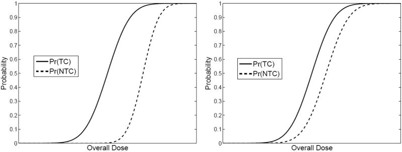
Schematic dose-response curves for two hypothetical treatment plans. Left: Probabilities of tumor control (TC) and normal-tissue complications (NTC) for a relatively effective plan. Right: Same for a less effective plan.

The curves in Fig. 1 are directly analogous to plots of true-positive fraction (probability of detection) and false-positive fraction (probability of false alarm) vs. a decision threshold in signal-detection problems [6]. It is an easy step to replot Fig. 1 as Pr(TC) vs. Pr(NTC) with the overall dose as a hidden parameter. This plot, initially introduced by Moore and Mendelsohn [31] and analyzed in ROC terms by Metz et al. [32], is referred to as the Therapy Operating Characteristic or TOC curve. The TOC curves corresponding to Fig. 1 are shown in Fig. 2. TOC curves were further studied by Andrews [33] who discussed how the TOC concept could be used for objective therapy optimization on a per-patient basis.

Figure 2.

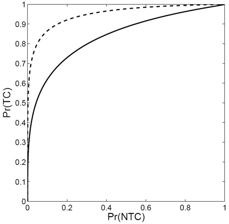
Therapy Operating Characteristic curves for the two treatment plans depicted in Fig. 1. The upper curve in this figure corresponds to the plan on the left in Fig. 1.

This paper uses the area under the TOC curve (AUTOC) as a figure of merit for radiation therapy planning and for the imaging components that affect the plan. An AUTOC of 1.0 is ideal, and the diagonal line with AUTOC = 0.5 corresponds to a treatment scenario in which the probability of tumor control can be increased only at the expense of an identical increase in the probability of normal-tissue complications. In contrast to ROC, an AUTOC ≪ 0.5 can also occur, in the case of a very bad treatment plan where there is a large probability of damage to normal tissues with little chance of tumor control.

In Sec. 2 we review the theory of TOC as originally laid out in [34]. In Sec. 3 we discuss some simplifying assumptions applicable to external-beam radiation therapy. In Sec. 4 we show how AUTOC can be used to evaluate segmentation algorithms, and in Sec. 5, we show how it can be used to evaluate the effect of patient motion on externalbeam radiation therapy. Application of the theory to the case where molecular-imaging data are included in the planning of external-beam radiotherapy is discussed in Sec. 6, and application to therapy with targeted internal radiation sources is illustrated in Sec. 7 by discussing therapy based on the human sodium iodine symporter.

In all of these applications, the theory is couched in the language of conditional probabilities and formally stated as high-dimensional nested integrals, starting with a fully general expression and then making reasonable assumptions to get tractable results. The assumptions are often stated conceptually in the form of high-dimensional delta functions, which should be regarded as devices for showing that certain integrals are unnecessary if the stated assumptions can be justified. In practice, all remaining integrals can be performed by Monte Carlo methods, and none of the integrals will have to be performed analytically.

We emphasize that it is not our intent to evaluate the effects of all possible sources of uncertainty in the radiation therapy process simultaneously, nor do we imply that the TOC is a complete measure of the efficacy of the therapy. Rather, in each of the sections that follow, we focus on one aspect of imaging in radiation therapy at a time and consider mainly the variability arising from the images, since they are the concern of this paper. If we have two or more competing approaches to the imaging task in question (e.g., different segmentation algorithms), this procedure will allow us to rank them in terms of AUTOC. We return to this point in Sec. 8 where we discuss how other sources of randomness might change this rank ordering.

For a worked example of how this formalism can be applied to the evaluation of segmentation methods, see [34].

2. General Theory

A key feature that sets tasks relevant to radiation therapy apart from other tasks used in OAIQ is the importance of boundaries. Given an image data set, the first step in the planning of external-beam therapy is to segment the images and estimate the boundaries of the tumor and of any nearby normal tissues that might be subject to damage from the therapy radiation. Then the treatment plan strives to maximize the radiation dose within the tumor boundary while minimizing the dose within the boundaries of sensitive normal tissues. When the planned therapy is administered, it is also important to assure that the boundaries of the tumor remain within the planned treatment volume. Therefore the main goal of this section is to determine the relation between the boundaries and the probabilities of tumor control and normaltissue complications.

The imaging system that provides the data used in boundary determination is modeled as a continuous-to-discrete (CD) mapping [6] where the object is a function of continuous variables and the image is a discrete set of numbers such as grey-level values at voxels. We assume that the tumor and all normal organs of interest have welldefined boundaries which can be represented as mathematical surfaces in a 3D space. For patient j, these surfaces are specified by a (potentially infinite) set of parameters denoted as B_j.

The surface descriptions contained in B_j are, of course, unknown, and it is the goal of a segmentation algorithm to estimate them in some way. The resulting estimate of the surfaces for patient j is denoted B̂_j. Unlike the continuous descriptions in B_j, the estimates in B̂_j specify a set of voxels or surface tesselations that define the surfaces in a discrete sense.

The data used for estimating the boundaries consist of one or more images. Typically, the normal-organ boundaries and the tumor boundaries will be estimated from a CT or MR image, but there is an increasing interest in including biological information estimated from PET images into the treatment planning process. For generality, we denote the available image data set for patient j as G_j, but we assume that this set must always include a CT study because x-ray attenuation data are needed for treatment planning.

From the estimated boundaries and the original CT data, a dosimetrist or physicist will derive a treatment plan which specifies the beam profiles, energies and exposures. Implementation of this plan will result in a dose distribution for patient j denoted D_j(r), where r is a three-dimensional position vector in the patient’s body. We assume that the dose distribution scales by the same factor at each position r as the exposure time or beam current is varied. If we assume further, for fractionated treatments, that the exposure is varied by the same proportion in each session, we can write

$$D_j\left(\mathbf{r}\right)=\alpha D_{0j}\left(\mathbf{r}\right),$$ (1)

where D_0j(r) is the dose distribution at some reference exposure and α is the ratio of an actual exposure to the reference exposure. Equivalently, we can say that D_0j(r) is the dose distribution for α = 1. For notational economy, we denote α D_0j(r) as D_j, with the dependence on α implicit.

One can think of α as setting the operating point on the TOC curve, hence setting the tradeoff between probability of tumor control and probability of occurrence of some specified normal tissue complication. It is important to note that the entire TOC curve is generated by varying α, so the shape of the TOC curve and the area under it are independent of α, though of course they depend on the spatial distribution of the dose. Thus α controls the abscissa in Fig. 1 but disappears in Fig. 2; instead any particular choice of the scale factor α determines one point on the TOC curve.

The stochastic quantities that control the probabilities of tumor control and normaltissue complications are noise in the image data; randomness in the estimated boundaries derived from a given image set; uncertainty in the actual delivered dose distribution, and of course the stochastic nature of the tissue response itself. We can describe all of these effects abstractly in terms of conditional probability density functions (PDFs).

The multivariate PDF for the image noise for patient j, denoted pr(G_j∣j), describes the effect of the noise in the raw projection data as propagated through the reconstruction algorithm. The conditioning on j implies that pr(G_j∣j) describes the stochastic variation of the images for hypothetical repeated imaging of the same patient with all imaging parameters (including the radiotracer distribution in the case of PET or SPECT) held constant; for much more on this PDF and copious references on the subject, see Chapter 15 of Barrett and Myers [6].

The PDF for the estimated boundaries given the image data, denoted pr(B̂_j∣G_j), would be a huge-dimensional delta function for an automatic segmentation algorithm because repeated trials with the same images would always deliver the same boundaries, but human analysts would not be so repeatable. We therefore retain pr(B̂_j∣G_j) as an unspecified PDF for now.

The PDF for the actual dose for patient j given the estimated boundaries and the image data is denoted pr(D_j∣B̂_j, G_j, j). The estimated boundaries B̂_j and the variations in x-ray attenuation coefficient in the CT data G_j determine the treatment plan and hence the intended dose distribution, but this PDF allows the actual dose to deviate in an unknown, random way from the intended one. The remaining conditioning on j allows for the response to depend on characteristics of the patient not captured in the image data and hence not considered in the calculations of probabilities of tumor control and normal-tissue complications.

Finally, the probability (not PDF) of tumor control, which depends on the actual dose distribution, the actual boundaries and possibly other biological factors such as oxygenation and perfusion, can be denoted Pr(TC∣D_j, B_j, j). The notation here is a trifle redundant because conditioning on the patient is implicitly specifying the true organ boundaries, but we retain the dependence on B_j to emphasize its importance.

With these definitions, we can apply elementary rules of conditional probability to write the probability of tumor control for patient j as

$$\begin{array}{c}\mathrm{Pr}(\mathit{TC}\mid \alpha ,j)=\\ \mathit{\int }d{\mathbf{D}}_j\mathit{\int }d{\widehat{\mathbf{B}}}_j\mathit{\int }d{\mathbf{G}}_j\mathrm{Pr}(\mathit{TC}\mid {\mathbf{D}}_j,{\mathbf{B}}_j,j)\mathrm{pr}({\mathbf{D}}_j\mid {\widehat{\mathbf{B}}}_j,{\mathbf{G}}_j,j)\mathrm{pr}({\widehat{\mathbf{B}}}_j\mid {\mathbf{G}}_j)\mathrm{pr}({\mathbf{G}}_j\mid j),\end{array}$$ (2)

where the dependence on α comes from (1).

Similarly, the general expression for the probability of normal-tissue complications is

$$\begin{array}{c}\mathrm{Pr}(\mathit{NTC}\mid \alpha ,j)=\\ \mathit{\int }d{\mathbf{D}}_j\mathit{\int }d{\widehat{\mathbf{B}}}_j\mathit{\int }d{\mathbf{G}}_j\mathrm{Pr}(\mathit{NTC}\mid {\mathbf{D}}_j,{\mathbf{B}}_j,j)\mathrm{pr}({\mathbf{D}}_j\mid {\widehat{\mathbf{B}}}_j,{\mathbf{G}}_j,j)\mathrm{pr}({\widehat{\mathbf{B}}}_j\mid {\mathbf{G}}_j)\mathrm{pr}({\mathbf{G}}_j\mid j).\end{array}$$ (3)

Note that the probabilities given by (2) and (3) ae determined by both the actual and the estimated boundaries; the estimated boundaries determine the treatment plan, but given a plan and hence a dose distribution, it is the actual boundaries, along with the overall dose α, that determine Pr(TC∣α, j) and Pr(NTC∣α, j).

3. Simplifications relevant to external-beam radiation therapy

The general equations (2) and (3) involve complicated, high-dimensional integrals, but fortunately we can make some simplifying assumptions. Consider first the conditional PDF pr(D_j∣B̂_j, G_j, j) which appears in (2) and (3). If we assume merely that the dosecalculation software is nonrandom, i.e., that it always returns the same computed dose distribution when it is rerun with the same estimated boundaries and image data, then this PDF must be a high-dimensional delta function.

Moreover, it is reasonable to neglect the potential inaccuracies in dose calculations and assume that the actual dose distribution, conditional on the estimated boundaries and the image data that go into the plan, is to a good approximation what the therapyplanning program says it is. There are two main justifications for this assumption. First, this critical aspect of radiotherapy has been widely studied, and the dose-computation algorithms have been continually refined and validated by Monte Carlo studies [35]. One can surely have confidence in them if an accurate image model is used. Second, the dose delivered by a beam of high-energy photons is rather non-local; a photon that undergoes a photoelectric or Compton interaction at a specific point in the tissue can deliver its dose over a range of a centimeter or more, and there are many such interactions, so noise or limited spatial resolution in the image may have little significant effect on the dose distribution.

The importance of this assumption is that we can eliminate one of the three integrals in (2) or (3). If there are no significant inaccuracies in dose calculation itself, conditional on the estimated boundaries and the image data, we can write

$$\mathrm{pr}({\mathbf{D}}_j\mid {\widehat{\mathbf{B}}}_j,{\mathbf{G}}_j,j)=\delta \left[{\mathbf{D}}_j-\mathbf{D}({\widehat{\mathbf{B}}}_j,{\mathbf{G}}_j)\right],$$ (4)

where D(B̂_j, G_j) is the dose distribution (interpreted as a function of continuous spatial variables) returned by the planning algorithm. The delta function can then be used to perform the integral over D_j, and (2) becomes

$$\mathrm{Pr}(\mathit{TC}\mid \alpha ,j)=\mathit{\int }d{\widehat{\mathbf{B}}}_j\mathit{\int }d{\mathbf{G}}_j\mathrm{Pr}\left[\mathit{TC}\mid \mathbf{D}({\widehat{\mathbf{B}}}_j,{\mathbf{G}}_j),{\mathbf{B}}_j,j\right]\mathrm{pr}({\widehat{\mathbf{B}}}_j\mid {\mathbf{G}}_j)\mathrm{pr}({\mathbf{G}}_j\mid j).$$ (5)

It is important to note that the probability of tumor control still depends on the actual patient boundaries B in this integral; our assumption of accurate dose calculation is conditional on the estimated boundaries, and it does not rule out additional dose-delivery errors from patient motion, incorrect patient positioning or inaccurate segmentation.

Another reasonable approximation is to neglect the patient-to-patient variation of tissue damage by ionizing radiation. As noted above, Pr(TC∣D_j, B_j, j) can depend on patient characteristics not captured by the image data; that was the reason for the final conditioning on j. In fact, we have littleway of knowingwhat these characteristics are in clinical practice, and we certainly could not incorporate them realistically in a simulation study. Thus we opt to delete the last j and write Pr(TC∣D_j, B_j, j) = Pr(TC∣D_j, B_j).

Now we note that the product of the last two conditional probabilities in (5) can be rewritten as a joint probability:

$$\mathrm{pr}({\widehat{\mathbf{B}}}_j\mid {\mathbf{G}}_j)\mathrm{pr}({\mathbf{G}}_j\mid j)=\mathrm{pr}({\widehat{\mathbf{B}}}_j,{\mathbf{G}}_j\mid j).$$ (6)

Thus (5) becomes

$$\mathrm{Pr}(\mathit{TC}\mid \alpha ,j)={\langle \mathrm{Pr}\left[\mathit{TC}\mid \mathbf{D}({\widehat{\mathbf{B}}}_j,{\mathbf{G}}_j),{\mathbf{B}}_j\right]\rangle }_{{\widehat{\mathbf{B}}}_j,{\mathbf{G}}_j},$$ (7)

where the notation indicates that the quantity in angle brackets is to be averaged over the joint distribution of the subscripted quantities, B̂_j and G_j.

4. Application to the evaluation of segmentation methods

Image segmentation can be performed manually by a human operator tracing boundaries on an image, or by an automated segmentation algorithm, or by an automated algorithm where the human intervenes to correct errors. These three options have analogies in the problem of lesion detection from images, where the detection can be performed entirely by a human, by a computer detection algorithm, or by a human in conjunction with an algorithm.

For the detection task, image quality is assessed by using a set of images, some of which contain one or more lesions and some contain no lesion. It is important to the evaluation that the true lesion status of each image be known to the experimenter, though of course this information is not given to the observer. The are two common methods for generating images with known truth; either the images can be completely simulated, or normal clinical images can be used with simulated lesions inserted into them. As simulation models get ever more realistic, the first option becomes more frequently the norm for lesion detection, and we assume here that image-segmentation methods will also be assessed from realistic simulated images. For a discussion of the evaluation of segmentation algorithms with clinical image and an example related to radiation therapy of the prostate, see [34].

The expression in (7) suggests a Monte Carlo algorithm that can be readily implemented with simulated data. Suppose we begin with an anatomical phantom to represent a particular patient j and we generate K random image samples, differing only by the realization of the Poisson noise in the raw projection data. The k^th such image sample is denoted ${\mathbf{G}}_j^{(k)}$ and the corresponding boundary estimate is denoted ${\widehat{\mathbf{B}}}_j^{(k)}$. The pair ( ${\widehat{\mathbf{B}}}_j^{(k)}$, ${\mathbf{G}}_j^{(k)}$) is a sample from the joint distribution pr(B̂_j, G_j∣j); only one index k is needed to specify the sample because ${\widehat{\mathbf{B}}}_j^{(k)}$ is generated directly (though not necessarily deterministically) from ${\mathbf{G}}_j^{(k)}$.

Because we started with an anatomical phantom, the true boundaries B_j are known, and we can use a standard therapy planning algorithm and standard TCP and NTCP modules to evaluate the quantity in angle brackets in (7). The Monte Carlo estimate of Pr(TC∣α, j) is then

$$\widehat{\mathrm{Pr}}(\mathit{TC}\mid \alpha ,j)=\frac{1}{K}\sum _{k=1}^K\mathrm{Pr}\left[\mathit{TC}\mid \mathbf{D}({\widehat{\mathbf{B}}}_j^{(k)},{\mathbf{G}}_j^{(k)}),{\mathbf{B}}_j\right],$$ (8)

where the probability on the righthand side is interpreted as the output of the TCP module. Similarly,

$$\widehat{\mathrm{Pr}}(\mathit{NTC}\mid \alpha ,j)=\frac{1}{K}\sum _{k=1}^K\mathrm{Pr}\left[\mathit{NTC}\mid \mathbf{D}({\widehat{\mathbf{B}}}_j^{(k)},{\mathbf{G}}_j^{(k)}),{\mathbf{B}}_j\right].$$ (9)

The Monte Carlo estimates of (8) and (9) are still functions of α, so the computation gives one point on the TOC curve. Repeating for several values of α as in an ROC study generates the TOC curve for phantom j; the study can be repeated for several phantoms to get an average TOC curve and AUTOC.

Evaluation of automatic segmentation algorithms is even easier. These algorithms are not random but they may yield erroneous boundaries, relative to the assumed gold standard. In estimation-theoretic terms, they have zero variance but nonzero bias. If algorithm m produces boundaries B̂_jm for patient j, Pr(TC) for that algorithm and patient is given by

$$\widehat{\mathrm{Pr}}(\mathit{TC}\mid \alpha ,j,m)=\mathrm{Pr}\left[\mathit{TC}\mid \mathbf{D}({\widehat{\mathbf{B}}}_{\mathit{jm}},{\mathbf{G}}_j),{\mathbf{B}}_j,j\right].$$ (10)

Again, this expression depends implicitly on α, and a similar expression holds for $\widehat{\mathrm{Pr}}(\mathit{NTC}\mid \alpha ,j,m)$, so a TOC curve specific to algorithm m and patient j is readily constructed. Averaging over patients then provides a task-based metric for the particular algorithm.

5. Application to patient motion

Now let’s go back to the general theory from Sec. 2 and see what assumptions should be made for purpose of evaluation of the effect of patient motion rather than segmentation algorithms. In this case we are not concerned with the effects of image noise or random segmentation algorithms, so the PDFs that describe those effects, pr(G_j∣j) and pr(B̂_j∣G_j), respectively, can be treated as delta functions in Eqs. (2) and (3). Equivalently, we can simply omit the integrals over G_j and B̂_j, so that (2) and (3) become

$$\mathrm{Pr}(\mathit{TC}\mid \alpha ,j)=\mathit{\int }d{\mathbf{D}}_j\mathrm{Pr}(\mathit{TC}\mid {\mathbf{D}}_j,{\mathbf{B}}_j,j)\mathrm{pr}({\mathbf{D}}_j\mid {\widehat{\mathbf{B}}}_j,{\mathbf{G}}_j,j).$$ (11)

$$\mathrm{Pr}(\mathit{NTC}\mid \alpha ,j)=\mathit{\int }d{\mathbf{D}}_j\mathrm{Pr}(\mathit{NTC}\mid {\mathbf{D}}_j,{\mathbf{B}}_j,j)\mathrm{pr}({\mathbf{D}}_j\mid {\widehat{\mathbf{B}}}_j,{\mathbf{G}}_j,j).$$ (12)

Another way of expressing these same results is to note that the true boundaries during therapy are some transformation of the original boundaries used in the treatment planning. Thus we write

$${\mathbf{B}}_j={\mathit{T}}_j{\widehat{\mathbf{B}}}_j,$$ (13)

where T_j is a transformation operator describing the motion and deformation of patient j. This transformation is, of course, random, and we describe it conceptually with a PDF pr(T_j). This introduces another integral in (11) and (12), so they become

$$\mathrm{Pr}(\mathit{TC}\mid \alpha ,j)=\mathit{\int }d{\mathbf{D}}_j\mathit{\int }d{\mathit{T}}_j\mathrm{Pr}(\mathit{TC}\mid {\mathbf{D}}_j,{\mathbf{B}}_j,j)\mathrm{pr}({\mathbf{D}}_j\mid {\widehat{\mathbf{B}}}_j,{\mathbf{G}}_j,{\mathit{T}}_j,j)\mathrm{pr}({\mathit{T}}_j).$$ (14)

$$\mathrm{Pr}(\mathit{NTC}\mid \alpha ,j)=\mathit{\int }d{\mathbf{D}}_j\mathit{\int }d{\mathit{T}}_j\mathrm{Pr}(\mathit{NTC}\mid {\mathbf{D}}_j,{\mathbf{B}}_j,j)\mathrm{pr}({\mathbf{D}}_j\mid {\widehat{\mathbf{B}}}_j,{\mathbf{G}}_j,{\mathit{T}}_j,j)\mathrm{pr}({\mathit{T}}_j).$$ (15)

To get back to a single integral, we assume, as in the segmentation case, that the dose-planning algorithm delivers accurate dose distributions based on the boundaries and CT data input to it. In the segmentation case, this assumption was expressed by (4), repeated here for convenience:

$$\mathrm{Pr}({\mathbf{D}}_j\mid {\widehat{\mathbf{B}}}_j,{\mathbf{G}}_j,j)=\delta \left[{\mathbf{D}}_j-\mathbf{D}({\widehat{\mathbf{B}}}_j,{\mathbf{G}}_j)\right],$$ (4)

where, as above, D(B̂_j, G_j) is the dose distribution (interpreted as a function of continuous spatial variables) returned by the planning algorithm. To apply this assumption to patient motion, however, we must recognize that the patient motion affects not only the boundaries but also the distribution of attenuation and scattering coefficients within the boundaries. With a slight abuse of notation, we will use the same operator T_j to describe the transformation of the CT values, so

$$\mathrm{pr}({\mathbf{D}}_j\mid {\widehat{\mathbf{B}}}_j,{\mathbf{G}}_j,j)=\delta \left[{\mathbf{D}}_j-\mathbf{D}({\mathit{T}}_j{\widehat{\mathbf{B}}}_j,{\mathit{T}}_j{\mathbf{G}}_j)\right],$$ (16)

The interpretation here is that D(T_jB̂_j, T_j, G_j) is the dose distribution computed by the planning algorithm with perfect knowledge of the boundaries and attenuation coefficient distribution of patient j after the deformation. In fact, for the purposes of the integrals in (14) and (15), it is rigorously correct to assume this perfect knowledge because we require the PDF pr(D_j∣B̂_j, G_j, T_j, j), which is conditional on T_j.

Now using (16) in (14) and (15), we obtain

$$\mathrm{Pr}(\mathit{TC}\mid \alpha ,j)=\mathit{\int }d{\mathit{T}}_j\mathrm{Pr}\left[\mathit{TC}\mid \mathbf{D}({\mathit{T}}_j{\widehat{\mathbf{B}}}_j,{\mathit{T}}_j{\mathbf{G}}_j)\right]\mathrm{pr}({\mathit{T}}_j).$$ (17)

$$\mathrm{Pr}(\mathit{NTC}\mid \alpha ,j)=\mathit{\int }d{\mathit{T}}_j\mathrm{Pr}\left[\mathit{NTC}\mid \mathbf{D}({\mathit{T}}_j{\widehat{\mathbf{B}}}_j,{\mathit{T}}_j{\mathbf{G}}_j)\right]\mathrm{pr}({\mathit{T}}_j).$$ (18)

As in Sec. 3, the expressions in (17) and (18) suggest a Monte Carlo algorithm that can be implemented with simulated patient motion.

Suppose we begin with a segmented CT image for a particular patient j and we generate K new segmented CT images by randomly sampling different transformation operators T_j according to some model of the motion. The k^th such transformation is denoted ${\mathit{T}}_j^{(k)}$. We plan the therapy on the basis of the untransformed CT and boundary data, but then we run the dose calculation with each of the transformed data sets, generating new dose distributions for each, and input each into the modules that calculate the TC and NTC probabilities.

The Monte Carlo estimate of Pr(TC∣α, j) is then

$$\widehat{\mathrm{Pr}}(\mathit{TC}\mid \alpha ,j)=\frac{1}{K}\sum _{k=1}^K\mathrm{Pr}\left[\mathit{TC}\mid \mathbf{D}({\mathit{T}}_j^{(k)}{\widehat{\mathbf{B}}}_j,{\mathit{T}}_j^{(k)}{\mathbf{G}}_j)\right],$$ (19)

where the probability on the righthand side is interpreted as the output of the TCP module for the k^th transformation of the CT and boundary data from patient j.

Similarly,

$$\widehat{\mathrm{Pr}}(\mathit{NTC}\mid \alpha ,j)=\frac{1}{K}\sum _{k=1}^K\mathrm{Pr}\left[\mathit{NTC}\mid \mathbf{D}({\mathit{T}}_j^{(k)}{\widehat{\mathbf{B}}}_j,{\mathit{T}}_j^{(k)}{\mathbf{G}}_j)\right].$$ (20)

The Monte Carlo estimates of (19) and (20) are still functions of α, so the computation gives one point on the TOC curve. Repeating for several values of α as in an ROC study generates the TOC curve for phantom j. Thus one can obtain a TOC curve and AUTOC specific to patient j (with the motion model perhaps reflecting how “wiggly” that patient is). The study can also be repeated for several patients to get an average TOC curve and AUTOC, and these average values can be used to assess the effectiveness of devices and algorithms for measuring and controlling patient motion.

To illustrate the application of the TOC concept to patient motion, assume that a CT image is acquired and used to produce a dose plan. If there were no patient motion, one could produce a TOC curve as described above with overall dose α as the hidden variable (see the “no patient motion” TOC curve in Fig. 3a). To compute the Monte Carlo estimate of Pr(TC∣α, j) and Pr(NTC∣α, j) we need to generate random samples of the motion operator T_j. The TOC operating points for a fixed α but for many realizations of T_j is shown as the “possible operating points” in Fig. 3a. The smaller this “cloud” of TOC operating points is, the less of an effect patient motion has on the dose plan. When we compute the TOC operating point using (19) and (20) we are averaging over patient motion to create (when α is used as a hidden variable) an average TOC curve (also shown inn Fig. 3a). Figure 3b shows an alternate description. For every realization of patient motion T_j, there is a separate TOC curve generated by varying α. The range of possible TOC curves is illustrated as at the shaded region in Fig. 3b. The goal of a motion compensation method is to reduce the size of the cloud of possible TOC curves which will, in turn, raise the average TOC curve. Note that the TOC curve with no patient motion does not change so a smaller cloud of possible TOC curves must result in a higher average TOC curve.

Figure 3.

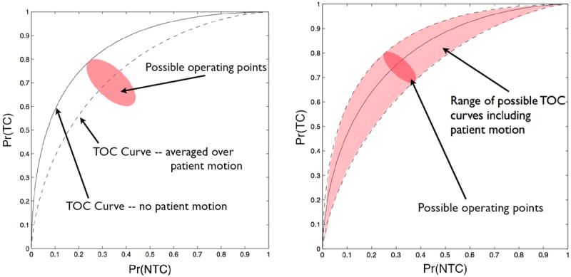
Illustrations of the effect of patient motion on a TOC curve.

So far we have assumed implicitly that the transformation is constant during a treatment, but if the motion model allows a time-varying deformation ${\mathit{T}}_j^{(k)}\left(t\right)$ – and if computer time is no obstacle – we can also define a time-averaged dose distribution as

$${\overline{\mathbf{D}}}_j^{(k)}\equiv \frac{1}{T}{\mathit{\int }}_0^T\mathit{dt}\mathbf{D}({\mathit{T}}_j^{(k)}(t){\widehat{\mathbf{B}}}_j,{\mathit{T}}_j^{(k)}(t){\mathbf{G}}_j),$$ (20)

where T is the treatment time. Of course, ${\overline{\mathbf{D}}}_j^{(k)}$ will be estimated in practice by a finite sum over discrete times rather than a continuous integral, and the dose calculation will have to be run for each time point.

With this modification, (19) becomes

$$\widehat{\mathrm{Pr}}(\mathit{TC}\mid \alpha ,j)=\frac{1}{K}\sum _{k=1}^K\mathrm{Pr}\left[\mathit{TC}\mid \alpha ,{\overline{\mathbf{D}}}_j^{(k)}\right],$$ (21)

and similarly for NTCP.

This expression is general enough to include the case where the beam profiles or other treatment parameters vary with time if we assume that the TCP and NTCP depend only on the total dose delivered and not on the dose rate. It could also be modified for the case where the patient was reimaged and the treatment replanned between fractions, though the required computer time increases with each such generalization.

Still another possible generalization is to build the motion model and all of this TOC formalism into the therapy planning process itself. If we have believable TCP and NTCP modules and enough computer power, we can conceivably use AUTOC as the objective function for therapy optimization.

6. Application to the use of molecular imaging in therapy planning

So far the only imaging modality we have considered explicitly is CT, but molecular imaging (MI) is also playing an increasingly important role in radiation therapy. For example, PET SPECT and EPR (electron paramagnetic resonance) imaging can be used to delineate the boundaries of hypoxic regions of a tumor [36-39], and MRI sequences sensitive to pH can be used to identify regions of rapid anaerobic growth [40-42]. In addition to gross tumor boundaries seen on CT, the boundaries of these subregions require special attention as part of the therapy planning.

The TOC formalism above is readily modified for the case where estimated boundaries obtained from molecular imaging are used in the therapy planning, either instead of or in addition to boundaries estimated from CT. For example, if both kinds of boundary estimates are used, and we assume that the noise in the two modalities as well as any errors in the boundary estimates from the two modalities are statistically independent, (5) becomes

$$\begin{array}{c}\mathrm{Pr}(\mathit{TC}\mid \alpha ,j)=\\ \mathit{\int }d{\widehat{\mathbf{B}}}_j^{\mathit{CT}}\mathit{\int }d{\widehat{\mathbf{B}}}_j^{\mathit{MI}}\mathit{\int }d{\mathbf{G}}_j^{\mathit{CT}}\mathit{\int }d{\mathbf{G}}_j^{\mathit{MI}}\mathrm{Pr}\left[\mathit{TC}\mid \mathbf{D}({\widehat{\mathbf{B}}}_j^{\mathit{CT}},{\widehat{\mathbf{B}}}_j^{\mathit{MI}},{\mathbf{G}}_j^{\mathit{CT}}),{\mathbf{B}}_j^{\mathit{CT}},{\mathbf{B}}_j^{\mathit{MI}},j\right]\\ \times \mathrm{pr}({\widehat{\mathbf{B}}}_j^{\mathit{CT}}\mid {\mathbf{G}}_j^{\mathit{CT}})\mathrm{pr}({\mathbf{G}}_j^{\mathit{CT}}\mid j)\mathrm{pr}({\widehat{\mathbf{B}}}_j^{\mathit{MI}}\mid {\mathbf{G}}_j^{\mathit{MI}})\mathrm{pr}({\mathbf{G}}_j^{\mathit{MI}}\mid j),\end{array}$$ (22)

where we have assumed that ${\mathbf{D}}_j=\mathbf{D}({\widehat{\mathbf{B}}}_j^{\mathit{CT}},{\widehat{\mathbf{B}}}_j^{\mathit{MI}},{\mathbf{G}}_j)$, as in (2) and (5). In other words, the dose distribution is fully determined by the estimated boundaries used as input to the treatment planning and the photon attenuation coefficients derived from CT, but in addition the probability of tumor control depends on the actual boundaries. A result similar to (22) applies to the probability of normal-tissue complications, and that result and (22) are sufficient to compute the TOC curve and AUTOC.

For the purpose of understanding the effect of MI on AUTOC, it is reasonable to assume that the segmentation algorithms used to estimate the boundaries are accurate, so that

$$\mathrm{pr}({\widehat{\mathbf{B}}}_j^{\mathit{CT}}\mid {\mathbf{G}}_j^{\mathit{CT}})=\delta [{\widehat{\mathbf{B}}}_j^{\mathit{CT}}-{\mathbf{B}}_j^{\mathit{CT}}];\mathrm{pr}({\widehat{\mathbf{B}}}_j^{\mathit{MI}}\mid {\mathbf{G}}_j^{\mathit{MI}})=\delta [{\widehat{\mathbf{B}}}_j^{\mathit{MI}}-{\mathbf{B}}_j^{\mathit{MI}}].$$ (23)

With these assumptions, (22) simplifies to

$$\mathrm{Pr}(\mathit{TC}\mid \alpha ,j)=\mathit{\int }d{\mathbf{G}}_j^{\mathit{CT}}\mathit{\int }d{\mathbf{G}}_j^{\mathit{MI}}\mathrm{Pr}\left[\mathit{TC}\mid {\mathbf{D}}_j,{\mathbf{B}}_j^{\mathit{CT}},{\mathbf{B}}_j^{\mathit{MI}},{\mathbf{G}}_j,j\right]\mathrm{pr}({\mathbf{G}}_j^{\mathit{CT}}\mid j)\mathrm{pr}({\mathbf{G}}_j^{\mathit{MI}}\mid j).$$ (24)

Because of the assumption that inaccuracies in boundary estimation are negligible, the only remaining random effects are the noise in the CT and MI images, represented by the two remaining integrals in (22). Of these two effects, only the CT noise affects Pr(TC∣α, j), and this effect arises only because the CT noise can affect the estimated photon attenuation coefficients that go into the planning algorithm. If we make the additional assumption that error in the attenuation coefficients can be neglected for the purpose of studying the impact of MI on AUTOC, we can omit these integrals and write

$$\mathrm{Pr}(\mathit{TC}\mid \alpha ,j)=\mathrm{Pr}\left[\mathit{TC}\mid \alpha {\mathbf{D}}_{0j},{\mathbf{B}}_j^{\mathit{CT}},{\mathbf{B}}_j^{\mathit{MI}},{\mathbf{G}}_j,j\right],$$ (25)

where we have used (1) to replace D_j with αD_0j. Similarly, we can write

$$\mathrm{Pr}(\mathit{NTC}\mid \alpha ,j)=\mathrm{Pr}\left[\mathit{NTC}\mid \alpha {\mathbf{D}}_{0j},{\mathbf{B}}_j^{\mathit{CT}},{\mathbf{B}}_j^{\mathit{MI}},{\mathbf{G}}_j,j\right].$$ (26)

With these results, it is now trivial to construct a TOC curve for patient j and compute AUTOC_j. We merely pick some nominal parameter settings and use the segmented CT and MI images in the treatment-planing program to get a baseline dose distribution D_0j. We can scale this dose by α to get αD_0j, which is then fed into the TCP and NTCP modules to yield Pr(TC∣α, j) and Pr(NTC∣α, j), respectively, for the particular patient j, the patient-specific treatment plan and the given value of α; varying α in this procedure then traces out the TOC cure with as many points as desired, and AUTOC for this patient and treatment plan is easily obtained by numerical integration.

If one wants to compare this AUTOC to the one that would be obtained without the use of the MI data, all that is required is to ignore the MI data and assume that the MI boundaries are the same as those obtained with the CT data.

7. Application to internal radiotherapy with the sodium iodide symporter

So far we have discussed only external-beam radiation therapy, but there is also considerable interest in methods where the radiation source is inside the body, as in brachytherapy, radioimmunotherapy and radiation therapy mediated by the human sodium iodide symporter gene, hNIS, which is the main topic of this section.

The hNIS protein [43-46] is used by the human thyroid gland to accumulate iodine from the blood stream as a substrate for synthesizing hormones such tetraiodothyronine (thyroxine). This highly efficient uptake of iodine is exploited through the use of raiolabelled iodine for both imaging and therapy of thyroid disease [47]. Although initially believed to be thyroid-sepcific, NIS detection in other tissues raised the possiblitiy for using this effective and safe modailty for the treatment of other cancer types. However, native levels of NIS in extrathyroidal tissues are not sufficient to mediate effective treatment [48]. As a result of this, many studies have investigated the potential for introduction of NIS expression to support imaging and treatment of a variety of cancer types. Broadly, these stuides are based on (1) attempts to upregulate native NIS expression through demethylation or stimulation with regulating agents [49,50], (2) direct introduction of NIS transgene expression into cancer cells using viral (detailed below) or non-viral vectors [51], or (3) the ‘Trojan horse’ approach, where cellular vehicles, such as Mesenchymal Stem Cells (MSCs), are engineered to express NIS, and then home to the tumor site for delivery of therapy [52, 53].

Successful migration of the MSCs to the tumor can be verified by SPECT imaging with ¹²³I or ^99mTc-pertechnetate, just as if the tumor were a human thyroid, and then the beta emitter ¹³¹I can be used for therapy, just as in clinical thyroid ablation therapy. Because ¹³¹I and ¹²³I are chemically identical, the therapy isotope and the imaging isotope must have the same spatial distribution.

Another way of using hNIS for internal radiation therapy is to inject genetically modified viruses such as adeno, measles, or other viral hosts that contain and express the hNIS gene. These viral constructs and engineered NIS expression can be made tumor- or tissue-specific by way of transcriptional targeting with tumor-specific promoters, thereby sparing non-target tissues from viral or radioiodide toxicities [43, 46]. Replication of the virus results in cytolysis, and this can also be controlled genetically through the use of tumor-specific promoter activity driving viral genes that are critical for assembly and release of active viral particles. The term ‘radiovirotherapy’ describes the synergistic results seen when cytolysis by use of a replication competent virus is also accompanied by NIS expression and radioiodine therapy [43, 54-56].

For hNIS-based radiotherapy with ¹³¹I, the image dataset must include both CT, to obtain the anatomical information needed for dose calculation, and a SPECT image with either pertechnetate or ¹²³I. Thus G_j refers to the set, { ${\mathbf{G}}_j^{\mathit{CT}}$, ${\mathbf{G}}_j^{\mathit{SPECT}}$}.

Given the imaging data for patient j, one must then estimate the distribution of the radiation dose D_j and from that compute PTC and PNTC. The most general integral expression for the probability of tumor control is [cf. (2)]

$$\begin{array}{c}\mathrm{Pr}(\mathit{TC}\mid \alpha ,j)=\\ \mathit{\int }d{\mathbf{D}}_j\mathit{\int }d{\mathbf{A}}_j^{\mathit{Tx}}\mathit{\int }d{\mathbf{G}}_j\mathrm{Pr}(\mathit{TC}\mid {\mathbf{D}}_j,j)\mathrm{pr}({\mathbf{D}}_j\mid {\mathbf{A}}_j^{\mathit{Tx}})\mathrm{pr}({\mathbf{A}}_j^{\mathit{Tx}}\mid {\mathbf{G}}_j)\mathrm{pr}({\mathbf{G}}_j\mid j),\end{array}$$ (27)

where ${\mathbf{A}}_j^{\mathit{Tx}}$ is the activity per unit volume of the therapy isotope, e.g., in MBq/cm³. The dependence on α is discussed below.

In (27), pr(G_j∣j) describes the noise in the image data; $\mathrm{pr}({\mathbf{A}}_j^{\mathit{Tx}}\mid {\mathbf{G}}_j)$ describes any errors or randomness is estimating the activity per unit volume of the therapy isotope from the SPECT data, and $\mathrm{pr}({\mathbf{D}}_j\mid {\mathbf{A}}_j^{\mathit{Tx}})$ similarly describes the inaccuracies or randomness in relating the activity per unit volume of the therapy isotope to the dose distribution (in grays). This step will be random as well as inaccurate if it is performed by a Monte Carlo algorithm [57]. The factor Pr(TC∣D_j, j) in (27) is just the output of the same tumor-response code as is used for external-beam therapy.

Once again, we can make some reasonable simplifying assumptions. First, if we neglect inaccuracy and randomness in the modules for computing TCP and NTCP, as we did in (4), we can omit the integral over D_j just by regarding D_j as the module output, $\mathbf{D}({\mathbf{A}}_j^{\mathit{Tx}})$.

The next factor to consider is the noise in the CT and SPECT images. If the noise is negligible, we can say formally that pr(G_j∣j) is a delta function, which is the same as simply omitting the integral over G_j as in Sec. 5.

The factor $\mathrm{pr}({\mathbf{A}}_j^{\mathit{Tx}}\mid {\mathbf{G}}_j)$ can be written as $\mathrm{pr}({\mathbf{A}}_j^{\mathit{Tx}}\mid {\mathbf{G}}_j^{\mathit{SPECT}})$ if the CT image is not used in the SPECT reconstruction, and for hNIS therapy with ¹²³I (but not for hNIS with pertechnetate or for radioimmunotherapy with surrogate SPECT agents), we have that

$${\mathbf{A}}_j^{\mathit{Tx}}=\alpha {\mathbf{A}}_j^{\mathit{SPECT}},$$ (28)

where α is the ratio of injected ¹³¹I activity to injected ¹²³I activity.

Thus $\mathrm{pr}({\mathbf{A}}_j^{\mathit{Tx}}\mid {\mathbf{G}}_j^{\mathit{SPECT}})$ describes any inaccuracy in measuring the ratio of injected activities as well as the error with estimating activity from a SPECT image. The estimation error arises from three main sources: collimator blur and scattering and attenuation of radiation in the patient’s body. Retaining this factor and the associated integral for now, we have

$$\mathrm{Pr}(\mathit{TC}\mid \alpha ,j)=\mathit{\int }d{\mathbf{A}}_j^{\mathit{Tx}}\mathrm{Pr}[\mathit{TC}\mid \mathbf{D}({\mathbf{A}}_j^{\mathit{Tx}})]\mathrm{pr}({\mathbf{A}}_j^{\mathit{Tx}}\mid {\mathbf{G}}_j^{\mathit{SPECT}}),$$ (29)

and, of course, similarly for Pr(NTC∣α, j).

If the objective of an image-quality study is to assess the impact of SPECT hardware or reconstruction algorithms on therapeutic efficacy as expressed by AUTOC, the integral in (29) can be evaluated by detailed, realistic Monte Carlo simulations. The index j in this case must refer to a particular simulated patient anatomy and pattern of radioiodine uptake. Averaging over simulated patients then gives an average TOC curve and an average AUTOC that can be used as figure of merit for image quality based on the efficacy of the hNIS-mediated therapy.

If, on the other hand, the quantitative accuracy of the SPECT reconstruction algorithm and the measurement of the activity ratio have been established, and the goal is to compute the TOC curve for a particular patient, we can write

$$\mathrm{Pr}(\mathit{TC}\mid \alpha ,j)=\mathrm{Pr}[\mathit{TC}\mid \mathbf{D}(\alpha {\mathbf{A}}_j^{\mathit{SPECT}})].$$ (30)

Thus, after calibration and validation studies, it should be possible to use the TCP/NTCP modules and the resulting TOC and AUTOC to assess and optimize the therapy for each patient.

8. Discussion and conclusions

All of the expressions given above for Pr(TC) and Pr(NTC) and their estimates are specific to a particular patient (or phantom), so we can generate a patient-specific TOC curve. For detection studies, by contrast, an ROC curve is defined only for a population of patients. To appreciate why this difference arises, we can go back to Fig. 1 which plots the probability of a beneficial outcome (tumor control) and an adverse outcome (normal-tissue complication) against a controllable variable (overall dose). The curves in Fig. 1 would apply directly to lesion detection if we simply interpreted the beneficial outcome as a true-positive detection, the adverse outcome as a false-positive detection and the controllable variable as the observer’s decision threshold.

For a given patient, we can define the TOC curve, the segmentation-averaged TOC curve, the motion-averaged TOC curve, and many more. In addition, we can then average these curves over patients to generate overall TOC curves that include patient variability. Thus, the TOC curve is a very general framework that can be used to assess the effect of these controls on therapeutic efficacy. One of the main differences between TOC and conventional ROC curves, is in the interpretation of the probabilities of adverse and beneficial outcomes. In the detection problem these probabilities are defined for some hypothetical ensemble of patients presenting for the same diagnostic study, but in the therapeutic problem the TCP and NTCP modules provide a way of computing the probabilities from knowledge of the actual delivered dose distribution and the true boundaries of the tumor and sensitive normal tissues.

It is also interesting to study what TOC curves teach us about ROC curves. Using a similar framework as we describe in this paper, it is possible to generate patient-specific ROC curves that assess the effects of, for example, image noise on the ability of the observer to detect an abnormality, in the well-known signal-known-exactly, backgroundknown-exactly (SKE/BKE) analysis. In other words, knowing the background and signal exactly is akin to imaging the same patient every time – only the image noise varies. To put it another way, the ROC curve for an SKE/BKE problem is very much like a TOC curve for a particular patient.

For purposes of image-quality assessment, the AUTOC figure of merit must be averaged over some group of patients or other subjects, including possibly simulated patients or animal subjects. Image quality is necessarily a statistical measure and cannot be determined based on the performance on a single patient. This immediately raises the question of assessing the systematic and random errors that affect the determination of AUTOC.

Among systematic errors, we must consider the TCP and NTCP modules themselves, which can be inaccurate because of oversimplified radiobiological models or uncertainty in the parameters that go into them. For the purpose of image-quality assessment, however, it is straightforward to see to what extent the modules influence our conclusions. Suppose, for example, that we are using AUTOC to compare segmentation algorithms, as suggested in [34]. Once we have the segmented images and have run the dose-planning algorithm for each, we can readily use many different TCP and NTCP modules and multiple choices of radiobiological parameters in each. If it turns out that the AUTOCs for segmentation algorithm A are consistently better than those for algorithm B, we can be confident in asserting that A is the method of choice for radiation therapy planning. On the other hand, we can also use the same segmented images and dose plans to generate TOC curves for different forms of normal-tissue complication; it may turn out that the choice of segmentation algorithm is different for different complications.

The most important random effect that arises in both the TOC and ROC approaches to task-based assessment of image quality is patient-to-patient variability. How many patients must one use to get a specified accuracy in estimates of the AUCs, and how can one assess the statistical significance of differences between the curves? This is a huge area of research in ROC analysis, stemming from seminal work by Charles Metz, Robert Wagner, Don Dorfman and many others. Similar analyses for TOC would be very useful.

Finally, though we have characterized the TOC curve as akin to an ROC for an individual patient, we can step back from the individual patient analysis and use a population-based TOC analysis to determine the marginal benefit provided by additional or improved imaging information. For example, we can compare AUTOC with and without molecular imaging information. This comparison can be carried out in the context of a cost-benefit analysis where the actual dollar cost of the molecular image is balanced against the reduced medical cost of improved cancer control and the reduction of the cost of treatment of normal tissue complication. In this context the TOC approach provides an algorithmic and relatively bias-free means by which to assess the ultimate social usefulness of an imaging modality. Studies might begin with animal model systems to which local image-guided therapies are applied.

References

- 1.Barrett HH. Objective assessment of image quality: Effects of quantum noise and object variability. Journal of the Optical Society of America A. 1990;7(7):1266–1278. doi: 10.1364/josaa.7.001266. [DOI] [PubMed] [Google Scholar]
- 2.Barrett HH, Denny JL, Wagner RF, Myers KJ. Objective assessment of image quality II: Fisher information, Fourier crosstalk, and figures of merit for task performance. Journal of the Optical Society of America A. 1995;12(5):834–852. doi: 10.1364/josaa.12.000834. [DOI] [PubMed] [Google Scholar]
- 3.Barrett HH, Abbey CK, Clarkson E. Objective assessment of image quality III: ROC metrics, ideal observers and likelihood-generating functions. Journal of the Optical Society of America A. 1998;15(6):1520–1535. doi: 10.1364/josaa.15.001520. [DOI] [PubMed] [Google Scholar]
- 4.Barrett HH, Myers KJ, Devaney N, Dainty JC. Objective assessment of image quality IV: Application to adaptive optics. Journal of the Optical Society of America A. 2006;23(12):3080–3105. doi: 10.1364/josaa.23.003080. [DOI] [PMC free article] [PubMed] [Google Scholar]
- 5.Caucci L, Barrett HH. Objective assessment of image quality V: Photon-counting detectors and list-mode data. Journal of the Optical Society of America A. 2012;29(6):1003–1016. doi: 10.1364/JOSAA.29.001003. [DOI] [PMC free article] [PubMed] [Google Scholar]
- 6.Barrettm HH, Myers KJ. Foundations of Image Science. John Wiley and sons; 2004. [Google Scholar]
- 7.Chakraborty Dev P, Berbaum Kevin S. Observer studies involving detection and localization: Modeling, analysis, and validation. Med Phys. 2004 Aug;31(8):2313–30. doi: 10.1118/1.1769352. [DOI] [PubMed] [Google Scholar]
- 8.Clarkson E. Estimation receiver operating characteristic curve and ideal observers for combined detection/estimation tasks. Journal of the Optical Society of America A. 2007;24(12):B91–98. doi: 10.1364/josaa.24.000b91. [DOI] [PMC free article] [PubMed] [Google Scholar]
- 9.Zelevsky MJ, Leibel SJ, Kutcher GJ, Fuks Z. Three-dimensional conformal radiotherapy and dose escalation: Where do we stand? Seminars in Radiation Oncology. 1998;8(2):107–114. doi: 10.1016/s1053-4296(98)80006-4. [DOI] [PubMed] [Google Scholar]
- 10.Eisbruch A. Intensity-modulated radiation therapy: A clinical perspective. Seminars in Radiation Oncology. 2002;12(3):197–282. doi: 10.1053/srao.2002.32430. [DOI] [PubMed] [Google Scholar]
- 11.Hatano K, Araki H, Sakai M, Kodama T, Tohyama N, Kawachi T, Imazeki M, Shimizu T, Iwase T, Shinozuka M, Ishigaki H. Current status of intensity-modulated radiation therapy (IMRT) International Journal of Clinical Oncology. 2007;12(6):408–415. doi: 10.1007/s10147-007-0703-9. [DOI] [PubMed] [Google Scholar]
- 12.Ahnesjo A, Hardemark B, Isacsson U, Montelius A. The IMRT information process–mastering the degrees of freedom in external beam therapy. Physics in Medicine and Biology. 2006;51(13):R381–R402. doi: 10.1088/0031-9155/51/13/R22. [DOI] [PubMed] [Google Scholar]
- 13.Jaffray DA. Image-guided radiation therapy: From concept to practice. Seminars in Radiation Oncology. 2007;17(4):243–305. doi: 10.1016/j.semradonc.2007.08.001. [DOI] [PubMed] [Google Scholar]
- 14.Chow JCL, Markel D, Jiang R. Technical note: Dose-volume histogram analysis in radiotherapy using the gaussian error function. Medical Physics. 2008;35(4):1398–1402. doi: 10.1118/1.2885373. [DOI] [PubMed] [Google Scholar]
- 15.Romeijn HE, Dempsey JF. Intensity modulated radiation therapy treatment plan optimization. TOP. 2008;16(2):215–243. [Google Scholar]
- 16.Wu Q, Mohan R, Niemierko A, Schmidt-Ullrich R. Optimization of intensity-modulated radiotherapy plans based on the equivalent uniform dose. International Journal of Radiation Oncology, Biology, Physics. 2002;52(1):224–235. doi: 10.1016/s0360-3016(01)02585-8. [DOI] [PubMed] [Google Scholar]
- 17.Stavrev P, Schinkel C, Stavreva N, Fallone BG. How well are clinical gross tumor volume DVHs approximated by an analytical function? Radiation and Oncology. 2009;43(2):132–135. [Google Scholar]
- 18.Deasy JO, El Naqa I. Radiation Oncology Advances. Chapter 11. Springer; 2008. Image-Based Modeling of Normal Tissue Complication Probability for Radiation Therapy. [PubMed] [Google Scholar]
- 19.Karger CP. Biological Models in Treatment Planning New Technologies in Radiation Oncology Springer. 2006;Chapter 18 [Google Scholar]
- 20.Kutcher Gerald J. Quantitative plan evaluation: Tcp/ntcp models. Frontiers of radiation therapy and oncology. 1996;29:67. doi: 10.1159/000424708. [DOI] [PubMed] [Google Scholar]
- 21.Park Clinton S, Kim Yongbok, Lee Nancy, Bucci Kara M, Quivey Jeanne M, Verhey Lynn J, Xia Ping. Method to account for dose fractionation in analysis of imrt plans: Modified equivalent uniform dose. International Journal of Radiation Oncology* Biology* Physics. 2005;62(3):925–932. doi: 10.1016/j.ijrobp.2004.11.039. [DOI] [PubMed] [Google Scholar]
- 22.Baumann M, Petersen Cordula. Tcp and ntcp: a basic introduction. Rays. 2005;30(2):99. [PubMed] [Google Scholar]
- 23.Stavrev P, Niemierko A, Stavreva N, Goitein M. The application of biological models to clinical data. Physica Medica. 2001;17(2):71–82. [Google Scholar]
- 24.Schultheiss Timothy E, Orton Colin G, Peck RA. Models in radiotherapy: volume effects. Medical physics. 1983;10:410. doi: 10.1118/1.595312. [DOI] [PubMed] [Google Scholar]
- 25.Niemierko Andrzej, Goitein Michael. Modeling of normal tissue response to radiation: the critical volume model. International Journal of Radiation Oncology* Biology* Physics. 1993;25(1):135–145. doi: 10.1016/0360-3016(93)90156-p. [DOI] [PubMed] [Google Scholar]
- 26.Lyman John T, Wolbarst Anthony B. Optimization of radiation therapy, iii: A method of assessing complication probabilities from dose-volume histograms. International Journal of Radiation Oncology* Biology* Physics. 1987;13(1):103–109. doi: 10.1016/0360-3016(87)90266-5. [DOI] [PubMed] [Google Scholar]
- 27.Lyman John T, Wolbarst Anthony B. Optimization of radiation therapy, iv: A dose-volume histogram reduction algorithm. International Journal of Radiation Oncology* Biology* Physics. 1989;17(2):433–436. doi: 10.1016/0360-3016(89)90462-8. [DOI] [PubMed] [Google Scholar]
- 28.Warkentin BJ, Field C, Stavrev P, Schinkel C, Stavreva N, Fallone BG. A TCP-NTCP estimation module using DVHs and known radiobiological models and parameter sets. Journal of Applied Clinical Medical Physics. 2004;5(1):50–63. doi: 10.1120/jacmp.v5i1.1970. [DOI] [PMC free article] [PubMed] [Google Scholar]
- 29.Gay HA, Niemierko A. A free program for calculating EUD-based NTCP and TCP in external beam radiotherapy. Physica Medica. 2007;23(3-4):115–125. doi: 10.1016/j.ejmp.2007.07.001. [DOI] [PubMed] [Google Scholar]
- 30.Sanchez-Nieto B, Nahum AE. Bioplan: Software for the biological evaluation of radiotherapy treatment plans. Medical Dosimetry. 2000;25(2):71–76. doi: 10.1016/s0958-3947(00)00031-5. [DOI] [PubMed] [Google Scholar]
- 31.Moore DH, II, Mendelsohn ML. Optimal treatment levels in cancer therapy. Cancer. 1972;30(1):97–106. doi: 10.1002/1097-0142(197207)30:1<97::aid-cncr2820300116>3.0.co;2-m. [DOI] [PubMed] [Google Scholar]
- 32.Metz CI, Tokars RP, Kronman HB, Griem ML. Maximum likelihood estimation of dose-response parameters for therapeutic operating characteristic (toc) analysis of carcinoma of the nasopharynx. International Journal of Radiation Oncology, Biology, Physics. 1982;8(7):1185–1192. doi: 10.1016/0360-3016(82)90066-9. [DOI] [PubMed] [Google Scholar]
- 33.Andrews J Robert. Benefit, risk, and optimization by roc analysis in cancer radiotherapy. International Journal of Radiation Oncology* Biology* Physics. 1985;11(8):1557–1562. doi: 10.1016/0360-3016(85)90345-1. [DOI] [PubMed] [Google Scholar]
- 34.Barrett HH, Wilson DW, Kupinski MA, Aguwa K, Ewell L, Hunter R, Mueller S. Therapy operating characteristic (TOC) curves and their application to the evaluation of segmentation algorithms. Proceedings of SPIE. 2010;7627:76270Z. doi: 10.1117/12.844189. [DOI] [PMC free article] [PubMed] [Google Scholar]
- 35.Chetty IJ, Curran B, Cygler JE, DeMarco G, Ezzell JJ, Faddegon BA, Kawrakow I, Keall PJ, Liu H, Ma CM, Rogers DW, Seuntjens J, Sheikh-Bagheri JV, Siebers D. Report of the aapm task group no. 105: Issues associated with clinical implementation of Monte Carlo-based photon and electron external beam treatment planning. Medical Physics. 2007;34(12):4818–4853. doi: 10.1118/1.2795842. [DOI] [PubMed] [Google Scholar]
- 36.Krohn Kenneth A, Link Jeanne M, Mason Ralph P. Molecular imaging of hypoxia. J Nucl Med. 2008 Jun;49(Suppl 2):129S–48S. doi: 10.2967/jnumed.107.045914. [DOI] [PubMed] [Google Scholar]
- 37.Halpern HJ, Yu C, Miroslav P, Barth E. Oxymetry deep in tissues with low-frequency electron paramagnetic resonance. Proceedings of the National Academy of Sciences of the United States of America. 1994;91(26):13047–13051. doi: 10.1073/pnas.91.26.13047. [DOI] [PMC free article] [PubMed] [Google Scholar]
- 38.Rischin Danny, Hicks Rodney J, Fisher Richard, Binns David, Corry June, Porceddu Sandro, Peters Lester J Trans-Tasman Radiation Oncology Group Study 98.02. Prognostic significance of [18f]-misonidazole positron emission tomography-detected tumor hypoxia in patients with advanced head and neck cancer randomly assigned to chemoradiation with or without tirapazamine: a substudy of trans-tasman radiation oncology group study 98.02. J Clin Oncol. 2006 May;24(13):2098–104. doi: 10.1200/JCO.2005.05.2878. [DOI] [PubMed] [Google Scholar]
- 39.Elas M, Bell R, Hleihel D, Barth ED, McFaul C, Haney CR, Bielanska J, Pustelny K, Ahn KH, Pelizzari CA. Electron paramagnetic resonance oxygen image hypoxic fraction plus radiation dose strongly correlates with tumor cure in FSa fibrosarcomas. International Journal of Radiation Oncology, Biology, Physics. 2008;71(2):542–549. doi: 10.1016/j.ijrobp.2008.02.022. [DOI] [PMC free article] [PubMed] [Google Scholar]
- 40.Raghunand N, Howison C, Sherry AD, Zhang S, Gillies RJ. Renal and systemic pH imaging by contrast-enhanced MRI. Magnetic Resonance in Medicine. 2003;49(2):249–257. doi: 10.1002/mrm.10347. [DOI] [PubMed] [Google Scholar]
- 41.Mori S, Eleff SM, Pilatus U, Mori N, VanZijl PCM. Sensitive detection of solventsaturable resonances by proton NMR spectroscopy: A new approach to study pH effects. Magnetic Resonance in Medicine. 1998;40(1):36–42. doi: 10.1002/mrm.1910400105. [DOI] [PubMed] [Google Scholar]
- 42.Ward KM, Balaban RS. Determination of pH using water protons and chemical exchange dependent saturation transfer (CEST) Magnetic Resonance in Medicine. 2000;44(5):799–802. doi: 10.1002/1522-2594(200011)44:5<799::aid-mrm18>3.0.co;2-s. [DOI] [PubMed] [Google Scholar]
- 43.Trujillo MA, Oneal M, Mcdonough S, Qin R, Morris JC. A probasin promoter, conditionally replicating adenovirus that expresses the sodium iodide symporter (NIS) for radiovirotherapy of prostate cancer. Gene Therapy. 2010;17(11):1325–1332. doi: 10.1038/gt.2010.63. [DOI] [PMC free article] [PubMed] [Google Scholar]
- 44.Gaut AW, Niu G, Krager KJ, Graham MM, Trask DK, Domann FE. Genetically targeted radiotherapy of head and neck squamous cell carcinoma using the sodium-iodide symporter (NIS) Head and Neck. 2004;26(3):265–271. doi: 10.1002/hed.10369. [DOI] [PubMed] [Google Scholar]
- 45.Dwyer RM, Schatz AM, Bergert ER, Myers RM, Harvey ME, Classic KL, Blanco MC, Frisk CS, Marler RJ, Davis BJ. A preclinical large animal model of adeonvirusmediated expression of the sodium-iodide symporter and potential in cancer therapy. Molecular Therapy. 2005;12(5):835–841. doi: 10.1016/j.ymthe.2005.05.013. [DOI] [PubMed] [Google Scholar]
- 46.Spitzweg C, Harrington KJ, Pinke LA, Vile RG, Morris JC. Clinical review 132: The sodium iodide symporter and its potential role in cancer therapy. Journal of Clinical Endocrinology and Metabolism. 2001;86(7):3327–3335. doi: 10.1210/jcem.86.7.7641. [DOI] [PubMed] [Google Scholar]
- 47.Dohan O, De La Vieja A, Paroder V, Riedel C, Artani M, Reed M, Ginter CS, Carrasco N. The sodium/iodide symporter (NIS): characterization, regulation, and medical significance. Endocrine Reviews. 2003;24(1):48–77. doi: 10.1210/er.2001-0029. [DOI] [PubMed] [Google Scholar]
- 48.Ryan J, Curran CE, Hennessy E, Newell J, Morris JC, Kerin MJ, Dwyer RM. The sodium iodide symporter (NIS) and potential regulators in normal, benign and malignant human breast tissue. PLoS One. 2011;6(1):e16023. doi: 10.1371/journal.pone.0016023. [DOI] [PMC free article] [PubMed] [Google Scholar]
- 49.Provenzano MJ, Fitzgerald MP, Krager KJ, Domann FE. Increased iodine uptake in thyroid carcinoma after treatment with sodium butyrate and decitabine (5-Aza-dC) Otolaryngology– head and neck surgery. 2007;137(5):722–728. doi: 10.1016/j.otohns.2007.07.030. [DOI] [PubMed] [Google Scholar]
- 50.Unterholzner S, Willhauck MJ, Cengic N, Schutz M, Goke B, Morris JC, Spitzweg C. Dexamethasone stimulation of retinoic acid-induced sodium iodide symporter expression and cytotoxicity of 131-i in breast cancer cells. Journal of Clinical Endocrinology and Metabolism. 2006;91(1):69–78. doi: 10.1210/jc.2005-0779. [DOI] [PubMed] [Google Scholar]
- 51.Klutz K, Russ V, Willhauck MJ, Wunderlich N, Zach C, Gildehaus FJ, Goke B, Wagner E, Ogris M, Spitzweg C. Targeted radioiodine therapy of neuroblastoma tumors following systemic nonviral delivery of the sodium iodide symporter gene. Clinical Cancer Research. 2009;15(19):6079–6086. doi: 10.1158/1078-0432.CCR-09-0851. [DOI] [PubMed] [Google Scholar]
- 52.Dwyer RM, Ryan J, Havelin RJ, Morris JC, Miller BW, Liu RM, Dwyer Z, Ryan J, Havelin RJ, Morris JC, Flavin C, O’Flatharta R, Foley MJ, Barrett HH, Murphy JM, Barry FP, O’Brien T, Kerin MJ. Mesenchymal stem cell-mediated delivery of the sodium iodide symporter supports radionuclide imaging and treatment of breast cancer. Stem Cells. 2011;29(7):1149–1157. doi: 10.1002/stem.665. [DOI] [PMC free article] [PubMed] [Google Scholar]
- 53.Knoop K, Kolokythas M, Klutz K, Willhauck MJ, Wunderlich N, Draganovici D, Zach C, Gildehaus FJ, Boning G, Goke B. Image-guided, tumor stroma-targeted 131i therapy of hepatocellular cancer after systemic mesenchymal stem cell-mediated NIS gene delivery. Molecular Therapy. 2011;19(9):1704–1713. doi: 10.1038/mt.2011.93. [DOI] [PMC free article] [PubMed] [Google Scholar]
- 54.Walrand S, Hanin FX, Pauwels S, Jamar F. Tumour control probability derived from dose distribution in homogeneous and heterogeneous models: Assuming similar pharmacokinetics, (125)Sn-(177)Lu is superior to (90)Y-(177)Lu in peptide receptor radiotherapy. Physics in Medicine and Biology. 2012;7(57):4263–4275. doi: 10.1088/0031-9155/57/13/4263. [DOI] [PubMed] [Google Scholar]
- 55.Dingli D, Diaz RM, Bergert ER, O’Connor MK, Morris SJ, Russel JC. Genetically targeted radiotherapy for multliple myeloma. Blood. 2003;102(2):489–496. doi: 10.1182/blood-2002-11-3390. [DOI] [PubMed] [Google Scholar]
- 56.Dwyer RM, Schatz SM, Bergert ER, Myers RM, Harvey ME, Classic KL, Blanco MC, Frisk CS, Marler RJ, Davis BJ, O’Connor MK, Russell SJ, Morris JC. A preclinical large animal model of adenovirus-mediated expression of the sodium-iodide symporter for radioiodide imaging and therapy of locally recurrent prostate cancer. Molecular Therapy. 2005;12(5):835–841. doi: 10.1016/j.ymthe.2005.05.013. [DOI] [PubMed] [Google Scholar]
- 57.El Naqa I, Pater P, Seuntjens J. Monte Carlo role in radiobiological modelling of radiotherapy outcomes. Physics in Medicine and Biology. 2012;57(11):R75–R97. doi: 10.1088/0031-9155/57/11/R75. [DOI] [PubMed] [Google Scholar]