

Abstract
When segmenting intraretinal layers from multiple optical coherence tomography (OCT) images forming a mosaic or a set of repeated scans, it is attractive to exploit the additional information from the overlapping areas rather than discarding it as redundant, especially in low contrast and noisy images. However, it is currently not clear how to effectively combine the multiple information sources available in the areas of overlap. In this paper, we propose a novel graph-theoretic method for multi-surface multi-field co-segmentation of intraretinal layers, assuring consistent segmentation of the fields across the overlapped areas. After 2-D en-face alignment, all the fields are segmented simultaneously, imposing a priori soft interfield-intrasurface constraints for each pair of overlapping fields. The constraints penalize deviations from the expected surface height differences, taken to be the depth-axis shifts that produce the maximum cross-correlation of pairwise-overlapped areas. The method’s accuracy and reproducibility are evaluated qualitatively and quantitatively on 212 OCT images (20 nine-field, 32 single-field acquisitions) from 26 patients with glaucoma. Qualitatively, the obtained thickness maps show no stitching artifacts, compared to pronounced stitches when the fields are segmented independently. Quantitatively, two ophthalmologists manually traced four intraretinal layers on 10 patients, and the average error (4.58±1.46 μm) was comparable to the average difference between the observers (5.86±1.72 μm). Furthermore, we show the benefit of the proposed approach in co-segmenting longitudinal scans. As opposed to segmenting layers in each of the fields independently, the proposed co-segmentation method obtains consistent segmentations across the overlapped areas, producing accurate, reproducible, and artifact-free results.
Index Terms: Graph theory, image co-segmentation, mosaicing, ophthalmology, retinal layer segmentation
I. Introduction
Optical coherence tomography (OCT) [1] has become an indispensable tool for 3-D imaging of the retina and its noninvasive assessment [2]. In particular, the condition of intraretinal layers are relevant to the diagnosis and management of a variety of ocular diseases such as age-related macular degeneration, diabetic-retinopathy, and glaucoma, the three most common causes of blindness in the developed world [3]. The layers are often affected by a disease, hence their accurate and reproducible segmentation, and quantitative thickness analysis, is of great clinical importance.
A limitation of currently commercially available OCT imaging devices is their scanning time. Thus, there is a trade-off between the acquired image spatial resolution and the imaged area. Clinical devices are optimized for relatively higher density smaller field of view (20°–30°) scanning. However, computing quantitative measures of retinal layers from a larger field of view (50° or more) may allow discovering new retinal biomarkers. Because large field of view devices are currently not clinically available, an alternative is to construct high density, large field of view mosaics, which is still acceptable to elderly patients.
The majority of efforts on enlarging retinal field of view have been in 2-D fundus photograph mosaicing, where the most prominent examples are [4]–[7]. There has been much less work on registration and mosaicing of retinal 3-D OCT images. In an early approach of Zawadzki et al. [8], they present a software application that allows a user to perform a 3-D translation of four OCT sub-volumes, and to combine them together into a larger, composite one. The first method for automated 3-D registration of OCT images was presented by Niemeijer et al. [9], where two images are aligned by a translation, based on 3-D scale-invariant feature transform (SIFT) keypoints. In [10], the same authors later proposed a two-stage registration method starting with a 2-D en-face registration guided by pre-segmented retinal vasculature, followed by 1-D translational alignment of A-scans along the depth-axis, obtained by the graph-search approach [11].
However, those works involved only pairs of images, while creating a multi-field mosaic is a more challenging problem. A method for mosaicing multiple OCT scans was presented for the first time by Li et al. [12]. There, the authors combine eight OCT fields by first jointly registering 2-D en-face projected OCT images. Once aligned in 2-D, they employ a first-order correction by shifting each OCT image along the z-axis. Layers are segmented independently on each individual OCT image field and are then pieced together to obtain stitched layer thickness maps.
To the best of our knowledge there has been no prior work on intraretinal layer co-segmentation of the OCT fields. In all of the main previously proposed segmentation methods [13]–[17], only individual OCT fields were considered. Regarding other modalities, a Bayesian approach was used in [18], where Markov random field prior encoded shared information to co-segment multiple magnetic resonance (MR) images. Recently [19] and [20], proposed a graph-theoretic methods for multi-modal co-segmentation of lesions from positron emission tomography (PET) and computed tomography (CT) based on graph cuts and random walk, respectively. However, there are no methods known to us for the co-segmentation of terrain-like surfaces from images of layered tissues.
In this work, we take a novel approach to layer segmentation of multi-field retinal OCT images. Instead of segmenting each field independently and then stitching the results together, the current state of the art, we propose a graph-theoretic layer segmentation method to perform simultaneous co-segmentation of all the fields involved, ensuring consistent segmentation in the overlapped areas. Such an approach is more robust, because it uses all the available image information, and will not produce seam artifacts in the resulting composite, stitched layer thickness maps. In addition, for 2-D en-face mutual alignment, instead of relying on low resolution, projected OCT images, we use simultaneously acquired scanning laser ophthalmoscopy (SLO) fundus images. Due to the salient texture present in SLO images, this allows us to benefit from a variety of computer vision techniques for mosaicing and panorama creation in general.
II. Methodology
The proposed methodology consists of two main steps. In the preprocessing step the imaged fields are aligned and resampled in the reference coordinate system. The alignment is en-face (x-y plane) only. Such 2-D aligned sets of images are then passed to the segmentation step where the surfaces of all the fields are co-segmented, taking into account the possible mutual displacements along the depth-direction (z-axis).
A. Preprocessing: 2-D En-Face Alignment
For 2-D en-face alignment of a set of M imaged fields , we employ a feature-based, affine registration, inspired by the image stitching workflow proposed in [6] and [21]. On each image, a set of keypoints is identified using SURF feature detector [22]. To mutually match the images, in all image pairs (Ii, Ij) we search for matching keypoints in the feature space. To estimate the pair-wise transformations robustly, we apply random sample consensus (RANSAC). A set of three matched keypoint pairs is randomly selected and the affine transformation Aij aligning them is computed, producing a set of inliers and outliers. The process is repeated multiple times, and the transformation producing the fewest number of outliers is chosen. Finally, the transformation Aij is reestimated from all the inliers using the least squares fit.
We then construct a connectivity graph with imaged fields as nodes and edges formed by the matched image pairs, with the edge cost being an inverse of the number of the inlier keypoints between the pair. If the resulting connectivity graph is disconnected, the mosaic is created from the images forming the largest connected subgraph. The image corresponding to the node that connects to the others with the smallest cost, is chosen as the reference. All the other images can then be aligned, and resampled onto the grid of the reference image via transformations Al, l ∈ {1, …, M}, obtained as a concatenation of transformations along the shortest path to the reference node in the graph.
Finally, we perform bundle adjustment [23] to solve for all of the transformation parameters jointly and to obtain global alignment. We follow the approach of [24], where for every 2-D point xk of the mosaic reference grid, the residual error ∈k across all aligned fields overlapping at xk is defined as
| (1) |
Where Ok is a set of overlapping pairs (i, j) ∈ Ok, such that xk is overlapped by the images Ii and Ij (Fig. 1). To obtain the global residual error, we iterate over all the points of the mosaic and compute . The parameters of Al, l ∈ {1, …, M}, are then optimized to produce the minimum global residual error, and are initialized with the values resulting from the alignment to the reference image. Such an approach ensures a uniform distribution of the misalignment error. Furthermore, computing residuals on the reference grid corresponds directly to the final perceived misalignment.
Fig. 1.

Residual error of a pair-wise alignment (red dotted line).
B. Multi-Surface Multi-Field Co-Segmentation
Given an integer N > 0 and M imaged fields, we want to co-segment an ordered set of N surfaces across the M fields. Surface Si is assumed to be positioned above the surface, Si+1, along the z-axis. We then pose the problem as finding the minimum of the following energy functional:
| (2) |
The term Eimage is the energy associated with how well a surface fits the underlying image information, i.e., a surface should lie along an intensity edge. The term Eshape incorporates prior shape information on spatial variation of a surface. The term Econtext incorporates prior pair-wise context information, i.e., the expected separation between neighboring pairs of surfaces. In this work, we specifically introduce the term Eoverlap to enforce a consistent surface co-segmentation in the areas where the fields overlap. The parameters, α, β, and γ weigh the contributions of the energy terms.
More specifically
| (3) |
| (4) |
| (5) |
| (6) |
where c(x, y, z) is an on-surface cost value, inversely proportional to the probability that the surface lies on that voxel. En-face voxel locations are denoted with p(x1, y1), q(x2, y2), and is a 2-D grid neighboring setting (four-neighborhood is assumed). Functions fs(·), fc(·), and fo(·) penalize deviations from the prior information. The following denote the differences in surface heights between locations. Δpq = S(p) − S(q) denotes the difference between neighboring locations p, of the same surface. denotes the difference between two neighboring surfaces at the same location. denotes the difference between the corresponding locations p ∈ Il and p ∈ Im in two overlapping fields of the same surface: . Finally, , , and are their a priori expected differences.
In order for the above functional to be optimally solvable in polynomial time, we adopt convex prior functions [25]. This is typically achieved by introducing the prior information in the form of hard [13] or soft [17], [26] constraints (Fig. 2). In our case, for Eshape and Econtext only hard constraints are used, as we will apply the co-segmentation to images of patients, the values and required by the soft-constraints were difficult to establish due to the large variability present in a patient population. For Eoverlap, we do expect segmentations to be consistent in the overlap areas, thus soft constraints are imposed.
Fig. 2.

Convex constraints: hard (in red), and soft (in blue). Shown separately (a), and combined (b).
For finding the optimal solution we build upon the graph-search framework [11], [27], [28], called LOGISMOS [29]. Each 3-D image I(x, y, z) of size, X × Y × Z, is oriented such that a terrain-like surface is defined as a function S: (x, y) → S(x, y), S(x, y) ∈ z = {0, …, Z−1}. Thus a terrain-like surface intersects each column of voxels p(x, y) at exactly one voxel (x, y, S(x, y)). The multi-surface segmentation task can be transformed into finding a minimum-cost closed set of the corresponding digraph. A closed set C in a digraph is a subset of nodes, such that all successors of any nodes in C are also contained in C. Surfaces then correspond to the upper envelope of the closed set. An advantage of the graph-search is that such a closed set can be optimally found efficiently, in a low-order polynomial time, by computing a minimum s-t cut in a derived arc-weighted digraph.
1) Graph Construction
A directed graph G = (V, E) is defined, with a set of nodes V and a set of arcs E. It is composed of M × N node-disjoint subgraphs Gm,n = (Vm,n, Em,n): m = 1, …, M; n = 1, …, N}, one for each field Im and each surface Sn. Every subgraph node vm,*(x, y, z) ∈ Vm,* one-to-one corresponds to image voxels Im(x, y, z). The cost wm,n(x, y, z) of a node is derived from image-based on-surface costs as
| (7) |
where costs of the nodes wm,n(x, y, 0) are set to a negative value to avoid the minimum-cost closed set being empty.
To impose the hard and soft constraints, the following arcs are constructed:
Intracolumn Arcs
To assure that a surface intersects the same voxel column p(x, y) only once, directed arcs are constructed from every node vm,n(x, y, z) | z > 0 to the node immediately below it vm,n(x, y, z−1). The arcs have +∞ weights, preventing them from being part of the min-cut.
Intercolumn Arcs
They implement the function fs(·) and enforce the shape of the surfaces to be smooth. The hard constraints are locally represented by two parameters, Δx and Δy, reflecting the allowed changes in surface height when moving from one neighboring surface point to the next in the x-direction and y-direction, respectively
| (8) |
| (9) |
The adjacent columns p(x, y) and p(x + 1, y) for every subgraph Gm,n are connected with +∞ weighted arcs, connecting node vm,n(x, y, z) ∈ p(x, y) to node vm,n(x + 1, y, max(z − Δx, 0)) ∈ p(x + 1, y), and vm,n(x + 1, y, z) ∈ p(x + 1, y) to node vm,n(x, y, max(z − Δx, 0)) ∈ p(x, y). It is analogously constructed for the y-direction.
Intrafield-Intersurface Arcs
To incorporate the prior context information fc(·), a set of arcs is constructed in-between the subgraphs Gm,n, Gm,n+1, of neighboring surfaces of the same field. We again impose hard-constraints, where the parameter denotes the maximum allowed surface distance between Sn and Sn+1, while denotes the minimum allowed one
| (10) |
The following directed arcs, with +∞ weights, are constructed between the nodes vm,n and vm,n+1 of the corresponding columns: vm,n(x, y, z) ∈ pn(x, y) to node and vm,n+1(x, y, z) ∈ pn+1(x, y) to node .
Interfield-Intrasurface Arcs
To implement fo(·), a set of arcs is constructed in-between subgraphs Gi,n and Gj,n, corresponding to a pair of overlapping fields of the same surface. In case more than two fields overlap, the construction is repeated for all the pairs of overlapping fields. To assure consistent segmentation of the surface in the overlapped area we use soft constraints, bounded by hard ones to limit the number of arcs and lower the computational burden. As the fields are aligned en-face but not along the z-axis, there is an expected column-specific shift between a pair of surfaces belonging to the overlapping pair of fields (Ii, Ij). First, we add the arcs with +∞ weights, imposing the hard constraint . The arcs connect vi,n(x, y, z) ∈ pi(x, y) to node and vj,n(x, y, z) ∈ pj(x, y) to node . Second we add the soft constraint, weighted-arcs in-between the hard constraint ones. For each , where , if [fo(h)]′ ≥ 0, an arc is added from vi,n(x, y, z) ∈ pi(x, y) to node with weight [fo(h)]″. If [fo(h)]′ ≤ 0, an arc is added from vj,n(x, y, z) ∈ qj(x, y) to node with the same weight [fo(h)]″. The [fo(h)]′ and [fo(h)]″ are the discrete equivalents of first and second derivative of fo, respectively [26].
The graph construction with the emphasis on the newly introduced interfield-intrasurface arcs is illustrated in Fig. 3.
Fig. 3.

Graph construction. (a) Example of two subgraphs Gi,n and Gj,n of the same surface Sn, with their intra and intercolumn arcs (in black), and interfield-intrasurface arcs (in red). Nodes belonging to the area of overlap are highlighted (in red). (b) Interfield-intrasurface arc construction in detail. Dashed arrows denote the arcs implementing soft constraints, solid arcs implement the hard constraints.
C. Application to Multi-Field OCT
1) Image Acquisition
To create an extended field of view, a nine-field acquisition was performed where a scanned subject sequentially fixates on spots ≈ 12.5° apart, forming a 3 × 3 grid pattern [Fig. 4(a)]. Acquisition was performed using the latest generation, commercially available, Spectralis OCT scanner (Heidelberg Engineering) using gaze tracking mode. The device acquires anisotropic 3-D OCT image (768 × 61 × 496 voxels, 12.41 × 132.22 × 3.87 μm3). In addition, immediately before the OCT acquisition, the device acquires confocal scanning laser ophthalmoscope (SLO), which provides isotropic 2-D fundus image (768 × 768 pixels, 12.41 × 12.41 μm2) of the same area, with a superior y-axis resolution (bold values) compared to OCT. The SLO fundus image and the OCT image are acquired through the same optics and are automatically co-registered by the device [Fig. 4(b)].
Fig. 4.

(a) Nine-field OCT acquisition: subject sequentially focuses on each point of a 3 × 3 grid. (b) Example of a macular SLO image (left) and the co-registered OCT projection image (right).
2) SLO Image Registration
For the 2-D en-face alignment of OCT images, we rely on the surrogate SLO fundus images. In addition to the higher spatial resolution there is more salient texture visible on the SLO [Fig. 4(b)], which facilitates the alignment. The transformations resulting from registration of SLO images are applied to the corresponding OCT images. The registration is limited to affine transformations to avoid nonlinear deformations of 3-D OCT images. In all pairs of SLO images, we search for matching keypoints (Fig. 5) in SURF descriptor space. The SURF descriptors are scale and rotation invariant, and relatively insensitive to changes in illumination, which is essential for robust feature matching. RANSAC is run with 1000 trials, thus even in case of low inlier probability (pin = 0.3), the probability that the correct transformation is not found would be very low (≈ 10−12). Since we do not expect the resulting transformations to modify the scale notably, if the scale change is larger than 5%, the transformation is considered unrealistic, and the image pair is left unmatched.
Fig. 5.

Automatically detected correspondence of keypoints obtained by SURF matching in two partially overlapping SLO images. Robustness to substantial illumination changes can be observed.
For the bundle adjustment, the nonlinear least squares optimization was performed with the Levenberg–Marquardt method, using the solver Ceres [30]. For computational speed-up we do not compute on ∈k every point of the reference grid but on a decimated 22 × 22 grid. An example of residual error distribution before and after the bundle adjustment is shown in Fig. 6. We can observe that before bundle adjustment the error is low over the central, reference image but can reach high values as we move toward the periphery. With bundle adjustment, the error becomes lower overall and is distributed more uniformly.
Fig. 6.

Local residual error of image alignment: (a) before and (b) after bundle adjustment.
3) Multi-Surface Segmentation
For multi-surface segmentation, we build upon the method for segmenting 11 intraretinal surfaces reported previously by our research group [31]. Due to large computational and memory requirements, the 11 intraretinal surfaces are not segmented simultaneously, but rather in a sequential and multiscale manner, in each step segmenting the surfaces lying in between the previously segmented ones [32]. As a preprocessing step to segmentation, each OCT image is independently flattened [13]. Flattening allows taking small regions-of-interest of the original OCT image for segmenting a particular set of surfaces, significantly reducing computational time and memory consumption. In addition, the surfaces of the flattened images have more consistent shapes. The flattening consists of approximate pre-segmentation of three surfaces in the downsampled image, and fitting a thin plate spline to the reference one. The image columns are subsequently aligned so that the reference surface becomes a flat plane at a predefined height. Thus, as a consequence of flattening, the overlapping images are approximately aligned along the z-axis. The pre-segmented surfaces are later re-estimated in the process of co-segmentation.
In this work, Eshape and Econtext implement the hard constraints only (E ∈ {0, +∞}), hence any positive value for the parameters α and β [in (2)] will produce the same result, we have set them to α = β = 1 for convenience. The remaining parameter γ is newly introduced and balances the contributions from Eimage and Eoverlap. Setting γ to 0 would result in each field being segmented independently. Setting γ to a very large value would impose hard constraints on the surface positions of overlapping fields, forcing them to be identical and reducing the method’s robustness to misregistrations. The optimal value for γ can not be known a priori but can be obtained by training-set performance optimization, as described in Section III-F.
The convex function implementing the soft constraint of Eoverlap [see (6)] is taken to be a quadratic function
| (11) |
The parameters σl,m and are specific to each overlapping pair of fields (Il, Im), and are estimated during the co-segmentation as follows. For an area of overlap of two fields, cross-correlation along the z-axis is computed and the point of maximum cross-correlation is selected to be . Finally, the σl,m is estimated from a quadratic fit to the positive part of the cross-correlation function (Fig. 7), whose half-width is used as the limiting hard-constraint parameter Hl,m.
Fig. 7.

Quadratic fit (in blue) to positive part (in-between the red lines) of the cross-correlation function (in black). Estimated σ = 8.8 voxels.
III. Evaluation Methodology
The performance of the proposed method was evaluated on 180 OCT images obtained from repeated nine-field acquisitions of 10 eyes (six right, four left) from 10 patients with glaucoma (three severe, five moderate, two mild). For comparison purposes all left-eye scans were mirrored to conform to the scans of the right eye. As the method is composed of two main elements: 2-D en-face alignment of SLO images and layer co-segmentation of the OCT images, we evaluate them separately and jointly, both qualitatively and quantitatively.
In addition, we compare the performance to the conventional approach where OCT fields are segmented independently. Statistical difference in the performance across the patients was evaluated with Wilcoxon signed-rank test, a paired test that does not assume normally distributed data. Statistical significance was assumed at p < 0.05.
To facilitate the evaluation and the visualization of the obtained wide-field layer thickness maps, a large field OCT image is created, which is composed of multiple disjoint regions (one for each field) stitched together. After 2-D alignment, the images are resampled, using the nearest neighbor interpolation, onto the grid of the reference OCT image. The seam lines of the composite image are carved using the Voronoi diagram. From a set of seeds sk, k ∈ {1, …, 9} representing the aligned image centers, for each seed we find a corresponding region Rk as consisting of all the points of the aligned image domain Ik that are closer to that seed than to any other
| (12) |
The carving process is illustrated in Fig. 8(a)–(c), where fast marching over each Ik is employed to obtain distances from the seeds.
Fig. 8.

Example of composite OCT image carving: (a) Frames of individual aligned images with their centers (circles). (b) Distance map from the image centers (seeds). (c) Resulting Voronoi diagram. (d) Projection image of the stitched, composite OCT, with overlayed B-scan selection for tracing. (e) B-scan of the flattened, composite OCT used for manual tracing, with the four surfaces overlayed.
A. En-Face Alignment Accuracy
To quantify the success of the 2-D en-face alignment, 10 visually prominent landmarks were identified on each overlapping pair of SLO images. Landmarks were mostly consisting of vascular bifurcations. As a measure of error, Euclidean distances were computed between the corresponding landmarks after the images were aligned. Accuracy is reported as the mean error ± the standard deviation across landmarks. In addition, we computed the accuracy separately for each of the nine fields to evaluate its spatial variation.
B. Co-Segmentation Accuracy
First, the difference in the results between the two segmentation approaches is evaluated qualitatively. Second, to quantitatively evaluate their accuracy, we compared the segmented surfaces to the manually traced ones. Two ophthalmologists independently traced on each patient a set of 10 B-scans, which equidistantly spanned the composite OCT image [Fig. 8(d)]. The following four retinal surfaces were traced [Fig. 8(e)]:
The inner limiting membrane (ILM).
Surface separating retinal nerve fiber layer (NFL) and ganglion cell layer (GCL).
Surface separating inner plexiform layer (IPL) and inner nuclear layer (INL).
The outer boundary of retinal pigment epithelium (RPE).
The four surfaces enable computing NFL, GCL+IPL, and the total retinal thickness, which are of primary clinical importance for evaluating glaucoma.
The manual tracings have been adjudicated by a third ophthalmologist. When the discrepancy between the two tracers resulted from their disagreement, the third ophthalmologist independently traced that B-scan. In total, this resulted in 17% of the B-scans being traced three times. Finally, the mean of the two most similar tracings was used as the gold standard surface.
C. Reproducibility
Reproducibility of the obtained layer thickness maps was evaluated with respect to the nine-field acquisition. The 10 patients had a repeated nine-field acquisition on the same day (≈ 20 min apart). The entire processing pipeline was rerun and the layer thicknesses obtained from the two acquisitions were compared. Thus, the reproducibility of the entire processing pipeline, including both the registration and the co-segmentation, was evaluated. The reproducibility was summarized as the mean ± standard deviation of the differences. In addition, to evaluate reproducibility of different areas of the retina, the differences were reported for 54 sectors distributed regularly over the wide 50° field of view.
D. Co-Segmentation of Longitudinal Scans
To show the potential of the proposed method in applications other than mosaicing, we applied our approach to the segmentation of scans of the same subject acquired at different moments in time. Macula-centered images were obtained from a separate set of 16 subjects that had a second scan acquired one month later, during which no structural changes were expected. The second scan was then registered to the first one, and the layers were segmented. The scans of the two time-points were manually traced by one ophthalmologist, and the obtained surfaces were taken as the gold standard. We then report the accuracy of segmentation on both time-points, and the longitudinal variability of the thickness maps produced by the two segmentation approaches.
E. Computational Resources
The nine-field segmentations were run on a multi-CPU Linux compute-server (2.5GHz AMD Opteron, 256GB RAM). The mean execution times and memory consumption are reported for both the co-segmentation and independent segmentation.
F. Estimation of the Parameter γ
To estimate the optimal value of γ in (2), additional nine-field acquisitions of five patients were used to form a training set. The set of the five patients was disjoint from the set of 10 used for evaluation and testing. One observer manually traced the four surfaces on a set of 10 B-scans per patient, which served as bronze standard. Co-segmentation was then run with a range of values of γ = {0.1, 0.5, 1, 5, 10, 50, 100} and compared with the bronze standard. The minimum mean unsigned error was obtained for γ = 1 (Fig. 9), which was then fixed and used throughout the evaluation and the results of the co-segmentation.
Fig. 9.

Selection of the parameter γ. Mean unsigned error across all surfaces and patients of the training set for different values of γ (in log scale).
IV. Results
A. En-Face Alignment Accuracy
For all the 10 patients, the central macular scan was identified as the reference image and all SLO images were succesfully aligned to form complete nine-field mosaics. An example of aligned and blended SLO images, with the landmarks, is shown in Fig. 10(a). Qualitatively, the image is sharp, with few ghost vessels, which is an indication of a good alignment. Quantitatively, the mean and the standard deviation of the error over all landmarks in the x-y plane was 3.5 ± 1.9 pixels (43.3 ± 23.4 μm). Error for each of the nine fields is given in Fig. 10(b)—showing only a slight decrease in peripheral accuracy compared to the central field location. The error in the peripheral areas can partly be contributed to the curved shape of the retina, which results in nonlinear transformation between the fields, not captured by the used affine one. However, errors seen on the SLO images are affecting less the actual OCT alignment, due to the much lower y-resolution of OCT (132.22 μm). Observing the stitched OCT image [Fig. 10(c)], the continuity of vascular structures is well preserved across the seams.
Fig. 10.

En-face alignment results: (a) SLO images blended by averaging, with manually denoted landmarks (in yellow). (b) Alignment error per field: mean (std) [SLO pixels]. (c) 2-D projection image of the corresponding stitched composite OCT.
B. Co-Segmentation Accuracy
Qualitative evaluation of the segmentation in three patients is shown in Fig. 11, where the proposed co-segmentation method is compared to the one where the fields are segmented independently. Fig. 11(a)–(d) shows on B-scans how the proposed segmentation becomes more robust and local errors are avoided. In Fig. 11(e) and (f) we give an example of NFL thickness map where independently segmenting the fields produced pronounced artifacts in the overlapped areas. Such inconsistencies are avoided when employing our new co-segmentation approach, obtaining artifact-free thickness maps.
Fig. 11.
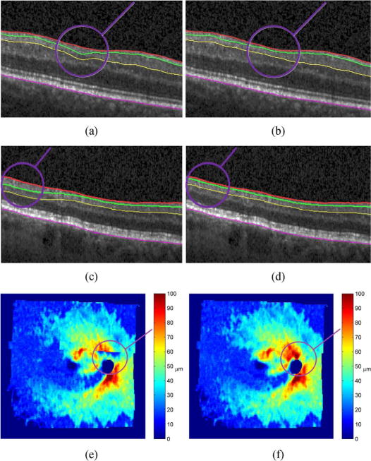
Three examples (different patients) of salient differences in the results when the segmentation is done without (a), (c), (e) and with (b), (d), (f) imposed layer consistency in the overlapped areas. Surface segmentation shown in a B-scan (a)–(d), and as a nine-field NFL thickness map (e), (f). The overlayed circles (in purple) denote the area of largest discrepancy between the two methods.
Quantitative performance of the co-segmentation, averaged per patient and compared to the expert-defined independent standard, is shown in Table I (unsigned errors). Clearly, the NFL-GCL boundary was the most difficult to segment, both automatically and manually. The mean unsigned error of 4.58 ± 1.46 μm is comparable to inter-observer variability of 5.86 ± 1.72 μm. The unsigned error for all four surfaces were significantly smaller (p < 0.05) than the corresponding inter-observer variabilities. The results are also comparable to the values reported by the state of the art, single-field segmentation methods [13], [17], [26] applied to macula-centered scans only. This shows that we are able to segment a larger field of view, while preserving the accuracy of the state of the art methods.
TABLE I.
Co-Segmentation Unsigned Surface Errors Expressed as mean ± std. [μm].(z-axis voxel spacing = 3.87 μm)
| Surface | Algo. vs. Avg. Obs. | Obs. 1 vs. Obs. 2 | Algo. vs. Obs. 1 | Algo. vs. Obs. 2 |
|---|---|---|---|---|
| ILM | 4.23±0.54 | 5.09±0.68 | 5.43±0.70 | 4.44±0.63 |
| NFL-GCL | 6.41±1.26 | 7.76±1.69 | 7.30±1.44 | 7.62±1.71 |
| IPL-INL | 4.75±0.48 | 6.44±0.84 | 6.29±0.84 | 5.22±0.51 |
| RPE | 2.92±0.42 | 4.14±0.71 | 3.75±0.71 | 3.45±0.49 |
|
| ||||
| Mean | 4.58±1.46 | 5.86±1.72 | 5.69±1.62 | 5.18±1.82 |
In comparison to the independent segmentation approach, the mean error as well as the NFL-GCL surface error obtained with the co-segmentation was consistently smaller (statistically significant). For other surfaces, the differences were not statistically significant between the two approaches. However, accurate segmentation of NFL-GCL is of high importance as the clinically relevant layers NFL and GCL+IPL are bounded by it. As a result, the thicknesses of the two layers were also more accurately obtained with co-segmentation (statistically significant). This difference between the two approaches across the 10 patients is shown in Fig. 12.
Fig. 12.

Unsigned errors for independent segmentation and co-segmentation. (a) NFL-GCL surface positioning errors and their per-subject means over the four surfaces. (b) NFL and GCL+IPL layer thickness errors. (a) Surface positioning error. (b) Layer thickness error.
C. Reproducibility
For qualitative evaluation of the reproducibility, an example of the three thickness map pairs obtained from two different acquisitions is shown in Fig. 13. No major discrepancies can be noted. Quantitative results per sectors are shown in Fig. 14. The majority of thickness discrepancies are in locations surrounding the optic nerve head, which is the most difficult area to segment. Overall mean differences per patient, for NFL thickness: 1.07 ± 0.35 μm, GCL+IPL thickness: 0.73 ±0.31 μm, and total retinal thickness: 1.86 ± 0.35 μm, were all below the z-axis image voxel spacing of 3.87 μm.
Fig. 13.

Retinal layer thickness reproducibility (first acquisition on the left, repeated on the right). NFL thickness (a), (b). GCL+IPL thickness (c), (d). Total retinal thickness (d), (e).
Fig. 14.

Mean regional layer thickness reproducibility values: (a) NFL, (b) GCL+IPL, and (c) the total retinal thickness.
Comparing the results to the ones obtained with independent segmentation (Fig. 15), the reproducibility of NFL layer was statistically significantly better, while the reproducibility of GCL+IPL was close to being significantly better (p = 0.06). There was no difference in reproducibility of the total retinal thickness, which is expected as the ILM and RPE surfaces are segmented with similar accuracy by both methods.
Fig. 15.

Layer thickness variability expressed as the mean unsigned difference between the two acquisitions for: NFL, GCL+IPL, and the total retinal thickness. (asterisk denotes statistically significant difference).
D. Co-Segmentation of Longitudinal Scans
Qualitative comparison of NFL thickness maps obtained with the co-segmentation and independent segmentation is shown in Fig. 16. Generally, in both cases the thickness maps from the two scans look similar, but the ones obtained with co-segmentation are less variable (more consistent), as expected. The superior performance of the co-segmentation is also proven quantitatively. The mean unsigned surface positioning error over all the surfaces was significantly smaller in both time-points (Fig. 17). In particular, the clinically important NFL-GCL surface was significantly more accurate for both time points while IPL-ONL surface was significantly more accurate for time-point #2 (p < 0.01) and close to being significantly better (p = 0.07) for time-point #1. Similarly, the consistency over the two time-points of all three layer thicknesses was significantly better (p < 0.01) for the co-segmentation approach (Fig. 18).
Fig. 16.

Example of NFL thickness variability (first acquisition on the left, second on the right), using independent segmentation (a), (b), and co-segmentation (c), (d). Arrows point to localized areas of discrepancy visible in panels (a), (b) and resolved in panels (c), (d).
Fig. 17.

Mean unsigned error over all the four surfaces for independent and co-segmentation for both time points (a) and (b). (a) Time-point #1. (b) Time-point #2.
Fig. 18.

Layer thickness variability of longitudinal scans expressed as the mean unsigned difference between the two scans for: NFL, GCL+IPL, and the total retinal thickness (asterisk denotes statistically significant difference).
E. Computational Resources
The mean execution times and memory consumption are presented in Table II. The numbers related to independent segmentation approach correspond to the case of segmenting the fields serially. Alternatively, independent segmentation of nine fields can be performed in parallel, which would decrease the execution time but increase the memory footprint by a factor of nine. In general, the resources required by a nine-field co-segmentation are much larger than those used by a single field segmentation. The constructed graph has nine times the number of nodes and additional large set of interfield-intrasurface arcs with the graph-search having polynomial computational complexity.
TABLE II.
Computational Resources Required Expressed as mean ± std
| Execution time [min] | Memory consumption [GB] | |
|---|---|---|
| 9-field Co-segmentation | 34.5±4.0 | 69.2±8.9 |
| 9-field Indep. segmentation | 9.8±1.7 | 3.6±0.2 |
| Single field segmentation | 1.1±0.2 | 3.6±0.2 |
V. Discussion
When multiple, spatially overlapping fields have to be segmented, a standard approach is to segment each of the fields individually and piece the information together. However, as each individual segmentation can produce a different result in the area of their overlap, such an approach can produce pronounced artifacts. As an alternative, we proposed a graph-theoretic method for multi-surface co-segmentation of the fields. The main contribution of our work is to utilize the multiply imaged structure and to impose a set of constraints that leads to a consistent and globally optimal surface segmentation over the entire set of overlapping image fields.
As a preprocessing step to multi-field co-segmentation, correspondences between the fields have to be established. The x-y plane, and z-axis correspondences were estimated separately. The low resolution along the y-axis of our anisotropic OCT dataset prohibited direct OCT-OCT registration. Thus, the 2-D en-face alignment of OCT was based on surrogate SLO images. Accuracy of scanner-provided registration between SLO and OCT was visually assessed as good [Fig. 4(b)]. Furthermore, SLO images display pronounced retinal texture, hence general purpose feature detectors could be applied to guide the alignment as opposed to using the vascular-based features only. For 1-D z-axis alignment, OCT has sufficiently high resolution and the layered structure of the retina facilitates the registration.
For multi-field co-segmentation, we build upon the graph-search framework, which is the current method of choice [13], [17], [26] for single-field intraretinal layer segmentation. Our method finds an optimal set of surfaces that satisfy soft and hard-constraints. To ensure consistency in the overlapped area, we benefit from recently introduced soft-constraints [17], [26]. Use of soft-constraints, due to additional arcs, does increase the computational requirements but it provides important robustness to potential z-axis misalignments as deviations from the expected shift [in (6)] are penalized, but not prohibited.
As opposed to previous works on intraretinal segmentation, here for the first time a method is evaluated on a large retinal field of view. Thus, even though we were able to segment a full set of 11 surfaces [31], denoting 10 intraretinal layers, to ease the effort of the manual tracing, the evaluation was focused on the four surfaces of main clinical value. In addition, we evaluated our method on images from glaucoma patients. Segmenting images of patients with severe glaucoma is particularly challenging as the NFL is often very thin or entirely missing, which explains why the NFL-GCL surface was the most difficult one to segment and to manually trace.
Compared to independent segmentation of the imaged fields, the proposed co-segmentation approach consistently performed better in both accuracy and reproducibility. The improvement was particularly pronounced in the segmentation of NFL-GCL surface. The NFL-GCL is difficult to segment as the interface between NFL and GCL layers is not always accompanied by a strong gradient and may even be completely missing. In those cases, the extra information available by having the same area multiply imaged can be utilized by the co-segmentation to achieve more robust results. For segmentation of surfaces where there is usually a strong intensity gradient present in the image (surfaces ILM and RPE), both segmentation approaches perform equally well.
The co-segmentation, as expected, does require more computational resources. This is mainly due to the large number of interfield-intrasurface arcs that are required to implement the soft-constraints, which make the geometric digraph more complex. A promising resource optimization step would be to avoid implementing dense 2-D spatial correspondences between overlapping subgraphs [red arcs in Fig. 3(a)] and to rely on a decimated subset of them. As the intraretinal surfaces are spatially smooth, the segmentation performance should not be affected while the graph complexity would be substantially decreased.
The main limitation of the proposed method is that although surface consistency across the fields is enforced, this does not guarantee consistency of layer thicknesses (distances between pairs of surfaces). Imposing layer thickness consistency directly across fields is a more difficult problem as it involves satisfying constraints of not just two, but four variables: . Such higher order, non-submodular functions do not have known transformations to max-flow min-cut problem on a graph, hence currently finding their optimum is intractable [33], and without known efficient algorithms. Alternatively, intersurface consistency could be enforced by additionally introducing a set of interfield-intersurface soft constraints. For intersurface soft-constraints, a priori information of expected distances between surfaces is required, which for our nonnormal, patient population was difficult to establish. Finally, the registration and segmentation are designed as two separate and independent steps, while ideally they would support each other in a joint registration-segmentation framework. How to achieve this while preserving the optimality of the solution is currently not clear.
The application of the proposed method was focused on co-segmentation of a nine-field OCT mosaic, but it is equally applicable to mosaics consisting of other tessellations, longitudinal scans, etc. Specifically, we gave an example of co-segmenting multiple longitudinal acquisitions of the same area, when no structural changes were expected. The resulting co-segmented surfaces were clearly more accurate and the thickness maps more consistent than when segmented independently. In general, there is an open question when the differences in longitudinal scans are due to acquisition variability and when due to the real change in the structure. One approach would be to use the knowledge of acquisition variability and to treat any larger differences as being structural. However, this would require using discontinuity preserving functions, which are nonconvex and do not allow finding optimal solution in polynomial time [33]. Overcoming the above limitations and applying the method to co-segmentation of longitudinal data with many time-points will be part of the future work.
VI. Conclusion
We have proposed a general method for simultaneous co-segmentation of multiple surfaces across multiple image fields that are spatially overlapped. To the best of our knowledge, this is the first such method for co-segmenting terrain-like surfaces in general and intraretinal layers in particular. Multi-surface co-segmentation is modeled as an energy minimization problem where a soft-constraint function penalizes segmentation inconsistencies in the overlapped areas. As all the energy terms are composed of convex functions, the problem can be transformed into one of finding a min s-t cut on a specially constructed arc-weighted digraph, which is optimally solvable in low order polynomial time. The method’s value has been demonstrated in the task of segmenting intraretinal layers from a set of overlapping OCT images, forming a wide field of view of the retina. In addition, we have shown its benefits when segmenting intraretinal layers from a set of repeated, single-field OCT scans. The results demonstrated that as opposed to segmenting layers in each of the fields independently, the current state of the art, the proposed co-segmentation method obtains consistent segmentation results across the overlapped and registered areas, producing more accurate, reproducible, and artifact-free results.
Acknowledgments
This work was supported in part by the National Institutes of Health (NIH) under Grant R01 EY019112, Grant R01 EY018853, and Grant R01 EB004640; in part by the National Science Foundation (NSF) under Grant CCF-0844765 and Grant CCF-1318996; in part by the Department of Veterans Affairs; and in part by the Marlene S. and Leonard A. Hadley Glaucoma Research Fund.
Footnotes
Color versions of one or more of the figures in this paper are available online at http://ieeexplore.ieee.org.
Contributor Information
Hrvoje Bogunović, Email: hrvoje-bogunovic@uiowa.edu, Department of Electrical and Computer Engineering, University of Iowa, Iowa City, IA 52242 USA.
Milan Sonka, Email: milan-sonka@uiowa.edu, Department of Electrical and Computer Engineering, the Department of Ophthalmology and Visual Sciences, and the Department of Radiation Oncology, University of Iowa, Iowa City, IA 52242 USA.
Young H. Kwon, Email: young-kwon@uiowa.edu, Department of Ophthalmology and Visual Sciences, University of Iowa, Iowa City, IA 52242 USA
Pavlina Kemp, Email: pavlina-kemp@uiowa.edu, Department of Ophthalmology and Visual Sciences, University of Iowa, Iowa City, IA 52242 USA.
Michael D. Abràmoff, Email: michael-abramoff@uiowa.edu, Department of Ophthalmology and Visual Sciences, the Department of Electrical and Computer Engineering, the Department of Biomedical Engineering, the University of Iowa, Iowa City, IA 52242 USA; VA Health Care System, Iowa City, IA 52246 USA.
Xiaodong Wu, Email: xiaodong-wu@uiowa.edu, Department of Electrical and Computer Engineering and the Department of Radiation Oncology, the University of Iowa, Iowa City, IA 52242 USA.
References
- 1.Huang D, Swanson EA, Lin CP, Schuman JS, Stinson WG, Chang W, Hee MR, Flotte T, Gregory K, Puliafito CA. Optical coherence tomography. Science. 1991 Nov;254(5035):1178–1181. doi: 10.1126/science.1957169. [DOI] [PMC free article] [PubMed] [Google Scholar]
- 2.Drexler W, Fujimoto JG. State-of-the-art retinal optical coherence tomography. Progr Retin Eye Res. 2008 Jan;27(1):45–88. doi: 10.1016/j.preteyeres.2007.07.005. [DOI] [PubMed] [Google Scholar]
- 3.Abramoff MD, Garvin MK, Sonka M. Retinal imaging and image analysis. IEEE Rev Biomed Eng. 2010 Jan;3(1):169–208. doi: 10.1109/RBME.2010.2084567. [DOI] [PMC free article] [PubMed] [Google Scholar]
- 4.Can A, Stewart C, Roysam B, Tanenbaum H. A feature-based technique for joint, linear estimation of high-order image-to-mosaic transformations: Mosaicing the curved human retina. IEEE Trans Pattern Anal Mach Intell. 2002 Mar;24(3):412–419. [Google Scholar]
- 5.Yang G, Stewart CV. Covariance-driven mosaic formation from sparsely-overlapping image sets with application to retinal image mosaicing; Proc IEEE Int Conf Comput Vis Pattern Recogn (CVPR); 2004. pp. 804–810. [Google Scholar]
- 6.Cattin PC, Bay H, Van Gool L, Szekely G. In: Larsen R, Nielsen M, Sporring J, editors. Retina mosaicing using local features; Proc Int Conf Med Imag Comput Comput Assist Interven (MICCAI); New York: Springer; 2006. pp. 185–192. [DOI] [PubMed] [Google Scholar]
- 7.Lee S, Reinhardt JM, Cattin PC, Abramoff MD. Objective and expert-independent validation of retinal image registration algorithms by a projective imaging distortion model. Med Image Anal. 2010 Aug;14(4):539–549. doi: 10.1016/j.media.2010.04.001. [DOI] [PubMed] [Google Scholar]
- 8.Zawadzki RJ, Fuller AR, Choi SS, Wiley DF, Hamann B, Werner JS. In: Manns F, Soderberg PG, Ho A, Stuck BE, Belkin M, editors. Improved representation of retinal data acquired with volumetric Fd-OCT: Co-registration, visualization, and reconstruction of a large field of view; Proc SPIE Ophthalmic Tech XVIII; 2008. p. 68440C. [Google Scholar]
- 9.Niemeijer M, Garvin MK, Lee K, Ginneken Bv, Abramoff MD, Sonka M. In: Pluim JPW, Dawant BM, editors. Registration of 3-D spectral OCT volumes using 3-D SIFT feature point matching; Proc SPIE Med Imag; 2009. p. 72591I. [Google Scholar]
- 10.Niemeijer M, Lee K, Garvin MK, Abràmoff MD, Sonka M. In: Abbey CK, Mello-Thoms CR, editors. Registration of 3-D spectral OCT volumes combining ICP with a graph-based approach; Proc SPIE Med Imag; 2012. p. 83141A. [Google Scholar]
- 11.Li K, Wu X, Chen DZ, Sonka M. Optimal surface segmentation in volumetric images-a graph-theoretic approach. IEEE Trans Pattern Anal Mach Intell. 2006 Jan;28(1):119–134. doi: 10.1109/TPAMI.2006.19. [DOI] [PMC free article] [PubMed] [Google Scholar]
- 12.Li Y, Gregori G, Lam BL, Rosenfeld PJ. Automatic montage of SD-OCT data sets. Opt Exp. 2011 Dec;19(27):26239–48. doi: 10.1364/OE.19.026239. [DOI] [PMC free article] [PubMed] [Google Scholar]
- 13.Garvin MK, Abramoff MD, Wu X, Russell SR, Burns TL, Sonka M. Automated 3-D intraretinal layer segmentation of macular spectral-domain optical coherence tomography images. IEEE Trans Med Imag. 2009 Sep;28(9):1436–1447. doi: 10.1109/TMI.2009.2016958. [DOI] [PMC free article] [PubMed] [Google Scholar]
- 14.Chiu SJ, Li XT, Nicholas P, Toth CA, Izatt JA, Farsiu S. Automatic segmentation of seven retinal layers in SDOCT images congruent with expert manual segmentation. Opt Exp. 2010 Aug;18(18):19413–28. doi: 10.1364/OE.18.019413. [DOI] [PMC free article] [PubMed] [Google Scholar]
- 15.Vermeer KA, van der Schoot J, Lemij HG, de Boer JF. Automated segmentation by pixel classification of retinal layers in ophthalmic OCT images. Biomed Opt Exp. 2011 Jun;2(6):1743–1756. doi: 10.1364/BOE.2.001743. [DOI] [PMC free article] [PubMed] [Google Scholar]
- 16.Kafieh R, Rabbani H, Abramoff MD, Sonka M. Intra-retinal layer segmentation of 3-D optical coherence tomography using coarse grained diffusion map. Med Image Anal. 2013 Dec;17(8):907–928. doi: 10.1016/j.media.2013.05.006. [DOI] [PMC free article] [PubMed] [Google Scholar]
- 17.Dufour PA, Ceklic L, Abdillahi H, Schroder S, Wolf-Schnurrbusch SDU, Kowal J. Graph-based multi-surface segmentation of OCT data using trained hard and soft constraints. IEEE Trans Med Imag. 2013 Mar;32(3):531–543. doi: 10.1109/TMI.2012.2225152. [DOI] [PubMed] [Google Scholar]
- 18.Xu J, Liang F, Gu L. Bayesian co-segmentation of multiple MR images; Proc IEEE Int Symp Biomed Imag; Jun. 2009; pp. 53–56. [Google Scholar]
- 19.Song Q, Bai J, Han D, Bhatia S, Sun W, Rockey W, Bayouth JE, Buatti JM, Wu X. Optimal co-segmentation of tumor in PET-CT images with context information. IEEE Trans Med Imag. 2013 Sep;32(9):1685–1697. doi: 10.1109/TMI.2013.2263388. [DOI] [PMC free article] [PubMed] [Google Scholar]
- 20.Bagci U, Udupa JK, Mendhiratta N, Foster B, Xu Z, Yao J, Chen X, Mollura DJ. Joint segmentation of anatomical and functional images: Applications in quantification of lesions from PET, PET-CT, MRI-PET, and MRI-PET-CT images. Med Image Anal. 2013;17(8):929–945. doi: 10.1016/j.media.2013.05.004. [DOI] [PMC free article] [PubMed] [Google Scholar]
- 21.Brown M, Lowe DG. Automatic panoramic image stitching using invariant features. Int J Comput Vis. 2006 Dec;74(1):59–73. [Google Scholar]
- 22.Bay H, Ess A, Tuytelaars T, Van Gool L. Speeded-Up Robust Features (SURF) Comput Vis Image Understand. 2008 Jun;110(3):346–359. [Google Scholar]
- 23.Triggs B, Mclauchlan PF, Hartley RI, Fitzgibbon AW. Bundle adjustment–A modern synthesis; Proc Int Workshop Vis Algorith: Theor Pract; 2000. pp. 298–375. [Google Scholar]
- 24.Marzotto R, Fusiello A, Murino V. High resolution video mosaicing with global alignment; Proc IEEE Int Conf Comput Vis Pattern Recogn; 2004. pp. 692–698. [Google Scholar]
- 25.Ishikawa H. Exact optimization for Markov random fields with convex priors. IEEE Trans Pattern Anal Mach Intell. 2003 Oct;25(10):1333–1336. [Google Scholar]
- 26.Song Q, Bai J, Garvin MK, Sonka M, Buatti JM, Wu X. Optimal multiple surface segmentation with shape and context priors. IEEE Trans Med Imag. 2013 Feb;32(2):376–386. doi: 10.1109/TMI.2012.2227120. [DOI] [PMC free article] [PubMed] [Google Scholar]
- 27.Wu X, Chen DZ. In: Widmayer P, Ruiz FT, Bueno RM, Hennessy M, Eidenbenz S, Conejo R, editors. Optimal net surface problems with applications; 29th Int Colloq Automata, Lang Programm; 2002. pp. 1029–1042. [Google Scholar]
- 28.Wu X, Chen DZ, Li K, Sonka M. The layered net surface problems in discrete geometry and medical image segmentation. Int J Comput Geom Appl. 2007 Jan;17(3):261–296. doi: 10.1142/S0218195907002331. [DOI] [PMC free article] [PubMed] [Google Scholar]
- 29.Yin Y, Zhang X, Williams R, Wu X, Anderson DD, Sonka M. LOGISMOS-layered optimal graph image segmentation of multiple objects and surfaces: Cartilage segmentation in the knee joint. IEEE Trans Med Imag. 2010 Dec;29(12):2023–2037. doi: 10.1109/TMI.2010.2058861. [DOI] [PMC free article] [PubMed] [Google Scholar]
- 30.Agarwal S, et al. Ceres Solver [Online] Available: https://code.google.com/p/ceres-solver/
- 31.Quellec G, Lee K, Dolejsi M, Garvin MK, Abramoff MD, Sonka M. Three-dimensional analysis of retinal layer texture: Identification of fluid-filled regions in SD-OCT of the macula. IEEE Trans Med Imag. 2010 Jun;29(6):1321–1330. doi: 10.1109/TMI.2010.2047023. [DOI] [PMC free article] [PubMed] [Google Scholar]
- 32.Lee K, Niemeijer M, Garvin MK, Kwon YH, Sonka M, Abramoff MD. Segmentation of the optic disc in 3-D OCT scans of the optic nerve head. IEEE Trans Med Imag. 2010 Jan;29(1):159–168. doi: 10.1109/TMI.2009.2031324. [DOI] [PMC free article] [PubMed] [Google Scholar]
- 33.Kolmogorov V, Zabih R. What energy functions can be minimized via graph cuts? IEEE Trans Pattern Anal Mach Intell. 2004 Feb;26(2):147–159. doi: 10.1109/TPAMI.2004.1262177. [DOI] [PubMed] [Google Scholar]