Sandwich corrected standard errors in family-based genome-wide association studies

Abstract

Given the availability of genotype and phenotype data collected in family members, the question arises which estimator ensures the most optimal use of such data in genome-wide scans. Using simulations, we compared the Unweighted Least Squares (ULS) and Maximum Likelihood (ML) procedures. The former is implemented in Plink and uses a sandwich correction to correct the standard errors for model misspecification of ignoring the clustering. The latter is implemented by fast linear mixed procedures and models explicitly the familial resemblance. However, as it commits to a background model limited to additive genetic and unshared environmental effects, it employs a misspecified model for traits with a shared environmental component. We considered the performance of the two procedures in terms of type I and type II error rates, with correct and incorrect model specification in ML. For traits characterized by moderate to large familial resemblance, using an ML procedure with a correctly specified model for the conditional familial covariance matrix should be the strategy of choice. The potential loss in power encountered by the sandwich corrected ULS procedure does not outweigh its computational convenience. Furthermore, the ML procedure was quite robust under model misspecification in the simulated settings and appreciably more powerful than the sandwich corrected ULS procedure. However, to correct for the effects of model misspecification in ML in circumstances other than those considered here, we propose to use a sandwich correction. We show that the sandwich correction can be formulated in terms of the fast ML method.

Introduction

Given the availability of large datasets of genotyped and phenotyped family members, it is of interest to determine which statistical test is most efficient in genome-wide association studies (GWAS), where computational efficiency and statistical power are important. One option is to use Plink,¹ which employs the standard Unweighted Least Squares (ULS) estimator in combination with the ULS sandwich^{2, 3} to correct the standard errors for the model misspecification of ignoring the clustering. This approach is non-iterative, and produces unbiased estimates and correct standard errors, without the need to specify a background covariance model. However, given clustered data, ULS is not necessarily the most powerful estimator.⁴ Maximum Likelihood (ML) is an important alternative, but is computationally more demanding. Fast algorithms have been developed, but these employ a model for the background covariance, which is limited to additive genetic and unshared environmental effects.^{5, 6} We note that shared environmental effects are often found in lifestyle and psychiatric phenotypes, such as substance use.^{7, 8, 9, 10} This raises a practical question: in conducting a family-based analysis, should one use the sandwich corrected ULS, which is fast, robust and requires no model to be specified for the background covariance matrix, or should one use ML, which is efficient and fast, provided one commits to a background model limited to additive genetic and unshared environmental effects? In the latter case, one may ask whether discarding shared environmental effects, affects the results of the ML procedure.¹¹

The present aim is to compare the ULS procedure with the ML procedure using simulated data. We consider the performance in terms of type I and type II error rates, with correct and incorrect background specification in ML. To correct for the effects of this misspecification, we propose to use a sandwich correction (as in Plink¹). We show that the sandwich correction can be formulated in terms of the fast ML method of Lippert et al.⁵

Materials and Methods

Family-based model for genetic association

Let y_ij be the vector of observed phenotypes, where subscript j stands for individual (j=1…n_i) and subscript i stands for family (i=1…N). Let g_ij be the vector of observed genetic markers coded as an additive genetic model, as 0 (aa), 1 (Aa) or 2 (AA).¹² We test the statistical association between each observed genetic marker and the phenotype in an appropriate regression model:

where b₀ represents the intercept, b₁ is the regression coefficient and ɛ_ij is the residual term. Let k equal 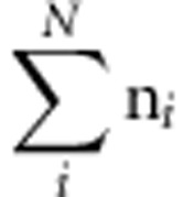, b^t equal the vector [b₀ b₁] and X equal the k × 2 matrix with the first column the unit vector, and the second, the k vector g containing the genetic information. Other covariates may be included, if desired (for example, age, sex). The k vector of residuals ɛ=y−Xb is normally distributed with k × k background covariance matrix V (positive definite), that is, ɛ|g∼N(0, V). We assume that V is block diagonal (but see Lippert et al,⁵ Pirinen et al⁶ and Visscher et al¹³), with diagonal blocks, V_i, representing the residual positive definite covariance matrix of each family. An advantage of retaining the full matrix V (and not reformulating the likelihood given the sparseness) is that the block diagonal structure can be relaxed to accommodate distant genetic relatedness.^{5, 6, 14} This makes the linear mixed approach very flexible. We assume that the elements in the diagonal blocks in V parameter vector θ contains the estimated elements of the conditional covariance matrix. Given MZ and DZ families, the covariance matrix V_i may be calculated conditional on zygosity, but otherwise unstructured and homoskedastic. We denote this the unstructured estimate of V(θ). Alternatively, V may be parameterized, that is, V(θ), where the parameter vector θ may contain shared (C) and unshared (E) environmental variance components (σ²_C, σ²_E), and additive (A) and dominance (D) variance components (σ²_A, σ²_D).^{15, 16} In this case, MZ and DZ relatedness is expressed in terms of these genetic variance components.

Estimation

We compare tests of b₁ based on ML estimation and ULS estimation, with regular and sandwich corrected standard errors. The log-likelihood function is:

where b represents the fixed effects, and θ the random effects.¹⁷ Maximization of the log-likelihood function subject to the correct specification of the background structure, yields the ML estimate of b, , which can be tested by means of the Wald test.^{4, 18} The parameterization of V(θ) in the linear mixed model, given family data, is well known.^{13, 19, 20, 21, 22, 23}

The ML estimator of b is based on solving b in the first order derivative of the ML function with respect to b:

If θ is unknown, this requires iteration. Note that the covariance matrix 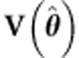can also be estimated once and then used as fixed in the generalized least squares estimator (see, for example, Pirinen et al⁶ and Li et al²⁴). The Wald test of b_1ML is based on . ULS is a special case with , that is, . The ULS estimator can be expressed as:^{4, 18, 25}

with

The ULS procedure involves misspecification in the case of family data, as 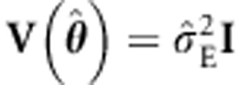is almost certainly incorrect. To correct the standard errors, we employ the sandwich correction of 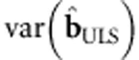,¹

We note that the sandwich correction is equally applicable to ML, given misspecified . For instance (eg, Dobson¹⁸):

where we employ the subscript m to denote misspecification.

Below we consider various tests of b₁ in family data of two full sibs and MZ and DZ twins with and without parents. First, we compare the ULS and ML procedures given correct specification of the background in ML, that is, θ=[σ²_A, σ²_E]. Specifically, we consider the standard ULS and ML procedures (ie, based on the so-called naive variance, which incorporates the assumption that the background model is correctly specified). We also consider the sandwich corrected ULS procedure (as in Plink¹) and the sandwich corrected ML procedure with the background V(θ) conditioned on zygosity, but otherwise unconstrained. That is, the family covariance matrix is freely estimated within the MZ and DZ families, which is consistent with the true model. We include the sandwich corrected ML procedure to investigate whether robustification does result in an overcorrection when the underlying model is in fact correct. Second, to assess the effects of misspecification, we consider standard ML estimation, with the (true) background θ=[σ²_A, σ²_C, σ²_E] misspecified as (a) , or as (b) . In addition, we use the misspecified 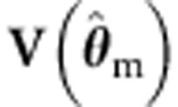with (and the misspecified with ) – estimated with standard ML using the incorrect background model – in the sandwich corrected ML procedure. We also include the standard and the sandwich corrected ULS procedures. Finally, we test b₁ using the standard ML procedure, with the background correctly parameterized (ie, estimating the variance components of the true model). We consider both the type I and type II error rates.

Simulation details

We generated family data for MZ and DZ families consisting of two sibs and MZ and DZ twins, with and without parents. Each simulated sample had a size of 4000 individuals. We simulated a diallelic genetic variant (GV) in Hardy-Weinberg equilibrium, with a minor allele frequency of 0.5, and explaining one percent (1%) of the phenotypic variance. We simulated the background covariance structure according to two models: (1) a model with additive (A) and unshared (E) environmental effects, that is, an AE model, θ=[σ²_A, σ²_E], with h²=σ²_A/(σ²_A+σ²_E) equal to 0.3, 0.5 or 0.7); (2) a model with additive genetic, shared (C) and unshared environmental effects, that is, an ACE model, θ=[σ²_A, σ²_C, σ²_E], with h²=σ²_A/σ²_ph=0.2, σ²_C/σ²_ph=0.6 and σ²_E/σ²_ph=0.2. We also considered an ACE model, with h²=σ²_A/σ²_ph=0.6, σ²_C/σ²_ph=0.2 and σ²_E/σ²_ph=0.2 (see Tables 2 and 3, Supplementary Material). These models were chosen to represent a range of complex phenotypes. For example, data generated based on the parameter values in the first cell of Table 1 are illustrative for family-based association studies of highly heritable traits such as height in adults,²⁶ whereas the data generated based on the parameter values in Table 3 may inform genome-wide analyses of ACE traits, such as initiation of substance use (eg, Vink et al⁷). We used the R package MASS²⁷ for data generation. We implemented the sandwich corrected ULS and the sandwich corrected ML procedures in R. We obtained the standard ML results using linear mixed modeling as implemented in the R-package nlme.²⁸ Observed power equals the proportion of datasets out of 10 000 replications, in which the P-value associated with the Wald test was smaller than our chosen alpha=10⁻⁷. Type I error rate was assessed at alpha=0.05, 0.01, 0.001 and 0.0001, using 1 000 000 datasets, simulated under the null hypothesis of b₁=0. Otherwise, given b₁≠0, we used 10 000 replications. Simulations were run on the Lisa Computer Cluster (www.surfsara.nl). The R script used to obtain the results is available at http://cameliaminica.nl/scripts.php.

Table 1. Power (alpha=10⁻⁷) and parameter estimates for the ML linear mixed (standard and sandwich corrected) and the ULS (standard and sandwich corrected) procedures.

Family structure	ML standard true model	Sandwich corrected ULS	Sandwich corrected ML (unstructured)	ULS standard
h2=70%
Two parents and four sibs
Mean (b1)	−0.141	−0.141	−0.141	−0.141
Mean (SE)	0.025	0.031	0.025	0.022
Mean (t-value)	−5.60	−4.62	−5.67	−6.35
Power	60.3	24.4	62.6	76.8
Four sibs
Mean (b1)	−0.141	−0.141	−0.141	−0.141
Mean (SE)	0.025	0.029	0.025	0.022
Mean (t-value)	−5.70	−4.95	−5.73	−6.35
Power	63.5	35.1	64.9	78.9
h2=50%
Two parents and four sibs
Mean (b1)	−0.141	−0.141	−0.141	−0.141
Mean (SE)	0.025	0.028	0.025	0.022
Mean (t-value)	−5.56	−4.96	−5.62	−6.34
Power	59.1	36.4	61.5	78.4
Four sibs
Mean (b1)	−0.141	−0.141	−0.141	−0.141
Mean (SE)	0.025	0.027	0.025	0.022
Mean (t-value)	−5.68	−5.25	−5.71	−6.34
Power	63.1	46.6	65.0	80.0
h2=30%
Two parents and four sibs
Mean (b1)	−0.141	−0.141	−0.141	−0.141
Mean (SE)	0.025	0.026	0.025	0.022
Mean (t-value)	−5.68	−5.40	−5.74	−6.34
Power	64.0	53.2	66.0	80.8
Four sibs
Mean (b1)	−0.142	−0.142	−0.142	−0.142
Mean (SE)	0.024	0.025	0.024	0.022
Mean (t-value)	−5.81	−5.63	−5.84	−6.36
Power	67.8	61.3	69.2	81.4

Abbreviations: ML, maximum likelihood; SE, standard error; ULS, unweighted least squares.

We simulated a genetic marker having an effect of 1% explained phenotypic variance and a minor allele frequency=0.5. The sample consisted of N=4000 individuals. The trait was simulated according to an AE background model (the true model) given various heritabilities (h²) (10 000 simulated samples for each cell). The background model in the ML procedure is correctly specified (true or saturated, ie, unstructured).

Table 3. Power (given alpha=10⁻⁷) and parameter estimates for the ML (standard and sandwich corrected) and the ULS (standard and sandwich corrected) procedures.

Family structure	ML standard ACE model (true)	ML standard AE model (false)	ML standard CE model (false)	Sandwich corrected ML (false: AE structured)	Sandwich corrected ML (false: CE structured)	ULS standard E model (false)	Sandwich corrected ULS E model (false)
Two parents and four sibs
Mean (b1)	−0.141	−0.141	−0.141	−0.141	−0.141	−0.141	−0.141
Mean (SE)	0.019	0.021	0.018	0.021	0.019	0.022	0.037
Mean (t-value)	−7.54	−6.59	−7.89	−6.6	−7.44	−6.33	−3.86
Power	98.6	89.4	99.2	89.4	98.1	73.0	7.5
Four sibs
Mean (b1)	−0.141	−0.141	−0.142	−0.141	−0.142	−0.141	−0.141
Mean (SE)	0.019	0.022	0.019	0.022	0.020	0.022	0.033
Mean (t-value)	−7.27	−6.49	−7.49	−6.50	−7.25	−6.36	−4.33
Power	97.4	88.1	98.2	88.0	97.1	75.9	16.4

Abbreviations: ML, maximum likelihood; SE, standard error; ULS, unweighted least squares.

The background model is (a) correctly specified (true) or (b) misspecified. Background covariance matrix was generated according to an ACE model (h²=0.2, c²=0.6). The genetic marker explained 1% phenotypic variance and had a minor allele frequency=0.5. The samples consisted of N=4000 individuals (10 000 simulated datasets per cell).

Results

Correctly specified background model: type I and type II error rates

First we checked the distribution of the four Wald tests given b₁=0, and the correct specification of the AE background, that is, θ=[σ²_A, σ²_E] (except standard ULS which assumes independence). As expected, the null distributions of the ML-based Wald tests (standard and sandwich corrected) and of the sandwich corrected ULS-based Wald test were correct (see Table 1, Supplementary Material). In contrast, the standard ULS procedure (without a sandwich correction) produced an excess of false positives. For instance, in the four sibs condition and with a 70% heritable trait, the observed type I error rate was 0.0024 given an alpha of 0.0001.

Given b₁=−0.141 (b₁ given the chosen effect size of 1%) and the correct specification of the AE background covariance matrix in ML (with h²=σ²_A/(σ²_A+σ²_E) equal to 0.3, 0.5 or 0.7), we obtained the results in Table 1 concerning the power to detect the GV effect.

The mean parameter estimates as produced by ML and ULS are equal, across all conditions. This is expected, as the estimators are all asymptotically unbiased and consistent.⁴ The standard errors as produced by the ML standard and by the sandwich corrected ML are identical. This is expected, as both procedures are based on the correct background covariance structure, be it correctly structured (ie, θ=[σ²_A, σ²_E]) or unstructured (the sandwich corrected ML). Therefore, the use of the sandwich does not result in any overcorrection. The ULS procedures are consistent, but differ in terms of power. The power of the standard ULS procedure appears to be greatest, but this is due to the fact that the standard errors are underestimated, as mentioned above. The sandwich corrected ULS procedure comes at a relative cost in terms of power (compared to ML). The loss in power increases with the family clustering due to the heritability of the trait. For example, in the four sibs condition, with a 70% heritable trait, the power of the sandwich corrected ULS procedure is 35.1%, whereas the power of the ML procedures is about 64%.

Besides the heritability of the trait, the size of the family cluster has a bearing on the power of ULS. For instance, given a 70% heritable trait, the difference in power between the ML and ULS with a sandwich correction is ∼30% and ∼35% when the sample consists of size 4 sibships and when it consists of two parents and four sibs, respectively (see Table 1). Note also the difference in power between the two robust methods as well (the sandwich corrected ULS and ML), with the power of the sandwich corrected ML procedure being higher.

Misspecified background model

We evaluated consequences on type I and II error rates of misspecifying the background model, V(θ). We employed a background model with additive genetic (σ²_A) and shared and unshared variance components (σ²_C and σ²_E), and discarded the effects of σ²_A (ML with an incorrect CE structured background) or σ²_C (ML with an incorrect AE structured background), or discarded both σ²_A and σ²_C (ULS with an incorrect E structured background). ML with a correctly specified background is also included. First we considered the type I error rates, given b₁=0. Table 2 contains the results.

Table 2. Type I error rates for the ML linear mixed (standard and sandwich corrected) and the ULS (standard and sandwich corrected) procedures.

Family structure	Alpha	ML standard ACE model (true)	ML standard AE model (false)	ML standard CE model (false)	Sandwich corrected ML (false: AE structured)	Sandwich corrected ML (false: CE structured)	ULS standard E model (false)	Sandwich corrected ULS E model (false)
Two parents and four sibs	0.05	0.049	0.049	0.06	0.05	0.049	0.2	0.051
	0.01	0.010	0.010	0.015	0.010	0.010	0.11	0.010
	0.001	0.0010	0.00097	0.0019	0.00097	0.0010	0.045	0.0011
	0.0001	0.0001	0.00009	0.0002	0.0001	0.00011	0.018	0.00012
Four sibs	0.05	0.05	0.05	0.057	0.05	0.05	0.18	0.05
	0.01	0.01	0.01	0.0127	0.01	0.01	0.08	0.01
	0.001	0.001	0.001	0.0014	0.001	0.001	0.025	0.001
	0.0001	0.0001	0.00012	0.00018	0.00012	0.00012	0.008	0.0001

Abbreviations: ML, maximum likelihood; ULS, unweighted least squares.

The background model is (a) correctly specified (true) or (b) misspecified. Background covariance matrix was generated according to an ACE model (h²=0.2, c²=0.6). The samples comprised 4000 individuals (1 000 000 simulated datasets per cell).

Based on these results, we conclude that the type I error rates of the ML procedure are not greatly affected by the misspecification. The misspecification is associated with a slight inflation (eg, 0.0002, given alpha=0.0001 in the two parents and four sibs cell), but the ML with the CE structured sandwich corrects this (0.00011). The misspecification hardly affects type I error rates. As expected, the standard ULS procedure 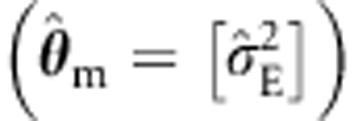produced incorrect type I error rates (for example, 0.008, given alpha=0.0001 in the four sibs cell). However, as above, the ULS sandwich correction yields correct type I rates. The ML with an ACE background is correctly specified and produces correct type I error rates.

Table 3 contains the results relating to the power given b₁≠0 and misspecified background. As expected, all modeling approaches yielded similar mean estimates of b₁, regardless of the specification of the background structure. Given correct background specification (θ=[σ²_A, σ²_C, σ²_E]) and sibships size 4, the power is about 97.4% (standard ML). The power of the standard ML procedure appears to increase to about 98.2%, when σ²_A is discarded , but this is spurious as it is due to the effect of the misspecification on the type I error (see Table 2). This effect is likely to be more noticeable at more stringent alpha levels (see also Minică et al²⁹). The ML with a CE structured sandwich, however, preserves the power equal to the power of the (true) ML ACE model, without inflating the type I error rate. Ignoring shared environmental effects, that is, dropping σ²_C in a θ=[σ²_A, σ²_C, σ²_E] model results in a loss in power. For instance, in the four sibs condition, the power of the standard ML procedure drops to about 88.1%, when σ²_C is discarded (similar results were obtained when dropping σ²_D in a θ=[σ²_A, σ²_D, σ²_E] model, where D stands for dominance; see Table 4 Supplementary Material). With an AE structured background, the standard errors as produced by the standard and the sandwich corrected ML are very similar, and so is the power. Given that the latter correctly reflects the parameter variance in the presence of a misspecified model, this result indicates that in the conditions considered here this type of misspecification does not affect estimation (ie, type I error rate is well controlled). However, this is not a general finding. Consider the extreme misspecification of the background employed by the ULS method. This has a clear effect, which is reflected in the notable discrepancy observed between the standard and the robust (correct) ULS standard errors (ie, 0.022 vs 0.033). Finally, although both are correct, we note that the sandwich corrected ML procedure is appreciably more powerful than the sandwich corrected ULS procedure (for example, power of 88.1% for the sandwich corrected ML with a misspecified AE structured background vs power of 16.4% for the sandwich corrected ULS procedure). Results follow similar trends in the samples consisting of two parents and four sibs.

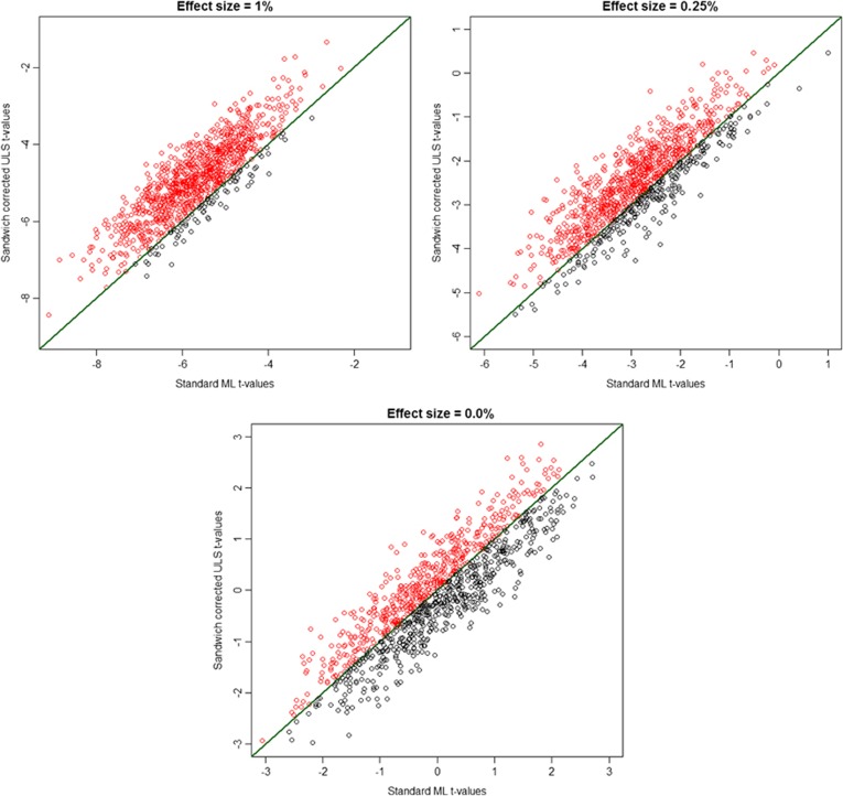
Given that these results pertain to averages over replications, we also looked at how often the ML t-values actually exceed the sandwich corrected ULS t-values, considering also the smaller effect sizes to be expected in GWAS. This might be of interest as it will provide an indication on how the two estimators are expected to perform in individual studies involving family data. Dots above the diagonal in Figure 1 show how often the ML-based Wald test is larger than the sandwich corrected ULS-based Wald test, given decline in the size of the genetic effect.

Figure 1.

Wald tests produced by the sandwich corrected ULS procedure compared with the test statistic obtained based on full information maximum-likelihood (standard ML) estimation method. We simulated 1000 datasets consisting of 500 MZ and 500 DZ four-sib families, and we varied the effect size of the genetic effect (1%, 0.25% and the null model). The heritability of the trait was h²=70%. The dots above the diagonal show the number of times the standard ML procedure produced a larger test statistic.

Figure 1 top left shows that the ML (true AE model) almost always produces a larger test statistic, when the effect size is relatively large (effect size of 1% explained phenotypic variance) and the sample is large enough to capture it. In the example, in just about 7.5% of the samples the sandwich corrected ULS test statistic was larger. However, as the effect size decreases, one can observe more and more sandwich corrected ULS-based Wald tests larger than those estimated by the ML procedure (as illustrated in Figure 1 top right). It can be seen that under the null model (Figure 1, bottom) no differences occur between the two estimation methods, which is as expected provided both are correct.

FaST-LMM formulation of the ML sandwich correction

The sandwich correction is computationally relatively simple and quick in the standard formulation of the linear mixed model. We note that the fast full information ML mixed procedures^{5, 6} are equally amenable to a sandwich correction. The ML sandwich can be presented as follows:

Given random effects , the background covariance matrix is reformulated as , where K is the genetic relationship matrix (positive semi-definite), I is the identity matrix and δ=σ_a²/σ_e². Lippert et al⁵ (see also Pirinen et al⁶) formulate the covariance matrix as follows:

where K=USU^t is the eigen value decomposition of K, with U, the eigenvectors, orthonormal, and S diagonal (eigenvalues). The matrix δ*I, being diagonal and constant, can be written as δ*UIU^t. The inverse is:

Note that the addition of off-diagonal terms in σ_e²*I, that is, terms accommodating shared environmental effects, would render the method invalid, as then the eigenvectors of the environmental covariance matrix cannot be chosen to equal U. In terms of this treatment of the matrix V(θ), the sandwich can be written:

In implementing this, the fact that (S+δ*I)⁻¹ is diagonal may be exploited to increase computational efficiency.

Discussion

We compared the standard and sandwich corrected ULS and ML procedures, in the context of family-based association analysis of a normally distributed phenotype. Conditional on the correct specification of the background, the standard ML procedure is appreciably more powerful than the sandwich corrected ULS procedure. The actual difference in power depends on the magnitude of the residual correlations, but increases with greater family resemblance.

We also considered the sensitivity of ML to model misspecification. Model misspecification involves the mismatch between the true background covariance model (say, an ACE or ADE trait) and the background model used in the analyses (a CE or AE model).

This may occur in using fast ML procedures, which employ the background covariance matrix necessarily limited to additive genetic (A) and unshared environmental (E) effects.^{5, 30} The standard ML procedure was quite robust under model misspecification in the simulated settings, and appreciably more powerful than the sandwich corrected ULS procedure. However, for circumstances other than those considered here, a sandwich correction is equally applicable to ML to correctly capture the parameter variance in the presence of model misspecification. The sandwich corrected standard errors may also be employed as a means to get an indication of the effects of background misspecification on the type I error rate (ie, the larger the discrepancy between the naive and sandwich corrected standard errors, the more likely the type I error rate of the procedure without a sandwich to be affected³¹).

In the present paper, we considered a normally distributed phenotype. Our conclusions apply equally to generalized linear modeling of binary traits, such as disease status. To demonstrate this, we included in the Supplementary Material (Supplementary Tables 5 and 6) results based on continuous and dichotomized (median – split) phenotypes. With respect to binary phenotypes, we note that a general (rather than generalized) linear model is often used in analyzing such variables (eg, Zhou and Stephens³²). Cogent arguments have been presented that the linear model may suffice in the analysis of binary phenotypes.^{5, 6}

Although relatively simple to implement and more efficient than the sandwich corrected ULS in correcting for model misspecification, to our knowledge the ML sandwich correction has not yet been implemented by any of the current software for GWAS that can handle family data. With respect to implementation, we note that generalized estimating equations (gee) procedure, as implemented in R³³ has four useful aspects. First, it has a choice of background models, which includes the independence model and exchangeable model (the latter is equivalent to the CE model in linear mixed modeling). Second, it includes sandwich corrected standard errors of the parameters b. Third, gee covers generalized linear model. Fourth, as gee is a library it can be accessed from Plink¹ and so provides a computationally feasible strategy for running genome-wide scans in family data. An annotated R script to do this is available at http://cameliaminica.nl/scripts.php.

In conclusion, for traits characterized by moderate to large familial resemblance, using ML with a correctly specified model for the familial covariance matrix should be the strategy of choice. For such traits, the potential loss in power encountered by the sandwich corrected ULS procedure does not outweigh its computational convenience. Using a fast ML algorithm that commits to a background model limited to additive and unshared environmental effects is acceptable even if shared environment has an influence on the phenotype of interest. That is, in the settings considered here, type I error rate of the standard ML was hardly affected by model misspecification. However, a sandwich correction is still of interest when employing ML in genome-wide scans, because (a) it produces correct standard errors regardless of whether the model is correctly parameterized or misspecified; hence it should be useful for situations other than those considered here, (b) it does not result in any overcorrection when the background model is in fact correctly specified, (c) as shown above, it is computationally cheap and can easily be incorporated in the fast ML procedures, and (d) it is a useful diagnostic tool for assessing model misspecification.³¹ Currently, Plink often is the preferred software when consortia share GWA results for meta-analyses. When including data from cohorts that include relatives, one should realize that the corrected standard errors while in many circumstances larger than the ML standard errors, are accurate, and so therefore are its type I and II error rates. For ordinary GWAS (ie, not family based), Plink is as good as FastLMM (as then ULS and ML are identical).

The authors declare no conflict of interest.

References

- Purcell S, Neale B, Todd-Brown K, et al. PLINK: a tool set for whole-genome association and population-based linkage analyses. Am J Hum Genet. 2007;81:559–575. doi: 10.1086/519795. [DOI] [PMC free article] [PubMed] [Google Scholar]
- Rogers WH. Regression standard errors in clustered samples. Stata Tech Bull. 1993;13:19–23. [Google Scholar]
- Williams RL. A note on robust variance estimation for cluster-correlated data. Biometrics. 2000;56:645–646. doi: 10.1111/j.0006-341x.2000.00645.x. [DOI] [PubMed] [Google Scholar]
- Greene WH. Econometric Analysis. India: Pearson Education; 2003. [Google Scholar]
- Lippert C, Listgarten J, Liu Y, Kadie CM, Davidson RI, Heckerman D. FaST linear mixed models for genome-wide association studies. Nat Meth. 2011;8:833–835. doi: 10.1038/nmeth.1681. [DOI] [PubMed] [Google Scholar]
- Pirinen M, Donnelly P, Spencer CCA. Efficient computation with a linear mixed model on large-scale data sets with applications to genetic studies. Ann Appl Stat. 2013;7:369–390. [Google Scholar]
- Vink JM, Wolters LMC, Neale MC, Boomsma DI. Heritability of cannabis initiation in Dutch adult twins. Addict Behav. 2010;35:172–174. doi: 10.1016/j.addbeh.2009.09.015. [DOI] [PMC free article] [PubMed] [Google Scholar]
- van den Bree MBM, Johnson EO, Neale MC, Pickens RW. Genetic and environmental influences on drug use and abuse/dependence in male and female twins. Drug Alcohol Depend. 1998;52:231–241. doi: 10.1016/s0376-8716(98)00101-x. [DOI] [PubMed] [Google Scholar]
- Kendler KS, Schmitt E, Aggen SH, Prescott CA. Genetic and environmental influences on alcohol, caffeine, cannabis, and nicotine use from early adolescence to middle adulthood. Arch Gen Psychiatry. 2008;65:674–682. doi: 10.1001/archpsyc.65.6.674. [DOI] [PMC free article] [PubMed] [Google Scholar]
- Vink J, Willemsen G, Boomsma D. Heritability of smoking initiation and nicotine dependence. Behav Genet. 2005;35:397–406. doi: 10.1007/s10519-004-1327-8. [DOI] [PubMed] [Google Scholar]
- Litière S, Alonso A, Molenberghs G. Type I and Type II error under random-effects misspecification in generalized linear mixed models. Biometrics. 2007;63:1038–1044. doi: 10.1111/j.1541-0420.2007.00782.x. [DOI] [PubMed] [Google Scholar]
- Falconer DS, Mackay TFC.Introduction to Quantitative Genetics4th ednHarlow: Pearson Education Limited; 1996 [Google Scholar]
- Visscher PM, Benyamin B, White I. The use of linear mixed models to estimate variance components from data on twin pairs by maximum likelihood. Twin Res Hum Genet. 2004;7:670–674. doi: 10.1375/1369052042663742. [DOI] [PubMed] [Google Scholar]
- Zaitlen N, Kraft P, Patterson N, et al. Using extended genealogy to estimate components of heritability for 23 quantitative and dichotomous traits. PLoS Genet. 2013;9:e1003520. doi: 10.1371/journal.pgen.1003520. [DOI] [PMC free article] [PubMed] [Google Scholar]
- Martin NG, Eaves LJ. The genetical analysis of covariance structure. Heredity (Edinb) 1977;38:79–95. doi: 10.1038/hdy.1977.9. [DOI] [PubMed] [Google Scholar]
- Eaves LJ. Inferring the causes of human variation. J Roy Stat Soc A. 1977;140:324–365. [Google Scholar]
- Pinheiro J, Bates D. Mixed-Effects Models in S and S-PLUS. New York: Springer; 2000. [Google Scholar]
- Dobson A. An Introduction to Generalized Linear Models. London: Chapman & Hall/CRC; 2002. [Google Scholar]
- Beem AL, Boomsma DI. Implementation of a combined association-linkage model for quantitative traits in linear mixed model procedures of statistical packages. Twin Res Hum Genet. 2006;9:325–333. doi: 10.1375/183242706777591272. [DOI] [PubMed] [Google Scholar]
- Guo G, Wang J. The mixed or multilevel model for behavior genetic analysis. Behav Genet. 2002;32:37–49. doi: 10.1023/a:1014455812027. [DOI] [PubMed] [Google Scholar]
- McArdle JJ, Prescott CA. Mixed-effects variance components models for biometric family analyses. Behav Genet. 2005;35:631–652. doi: 10.1007/s10519-005-2868-1. [DOI] [PubMed] [Google Scholar]
- Rabe-Hesketh S, Skrondal A, Gjessing HK. Biometrical modeling of twin and family data using standard mixed model software. Biometrics. 2008;64:280–288. doi: 10.1111/j.1541-0420.2007.00803.x. [DOI] [PubMed] [Google Scholar]
- van den Oord E. Estimating effects of latent and measured genotypes in multilevel models. Stat Methods Med Res. 2001;10:393–407. doi: 10.1177/096228020101000603. [DOI] [PubMed] [Google Scholar]
- Li X, Basu S, Miller MB, Iacono WG, McGue M. A rapid generalized least squares model for a genome-wide quantitative trait association analysis in families. Hum Hered. 2011;71:67–82. doi: 10.1159/000324839. [DOI] [PMC free article] [PubMed] [Google Scholar]
- Draper NR, Smith H. Applied Regression Analysis. New York: John Wiley and Sons; 1981. [Google Scholar]
- Silventoinen K, Sammalisto S, Perola M, et al. Heritability of adult body height: a comparative study of twin cohorts in eight countries. Twin Res Hum Genet. 2003;6:399–408. doi: 10.1375/136905203770326402. [DOI] [PubMed] [Google Scholar]
- Venables WN, Ripley BD.Modern Applied Statistics with S4th ednNew York: Springer; 2002 [Google Scholar]
- Pinheiro J, Bates D, DebRoy S, Sarkar D, Team RC.nlme: Linear and Nonlinear Mixed Effects ModelsR package version 3.1-111.2013
- Minică C, Dolan C, Hottenga J-J, Willemsen G, Vink J, Boomsma D. The use of imputed sibling genotypes in sibship-based association analysis: on modeling alternatives, power and model misspecification. Behav Genet. 2013;43:254–266. doi: 10.1007/s10519-013-9590-1. [DOI] [PubMed] [Google Scholar]
- Abecasis GR, Cherny SS, Cookson WO, Cardon LR. Merlin - rapid analysis of dense genetic maps using sparse gene flow trees. Nat Genet. 2002;30:97–101. doi: 10.1038/ng786. [DOI] [PubMed] [Google Scholar]
- Chavance M, Escolano S.Misspecification of the covariance structure in generalized linear mixed models Stat Methods Med Res 2012. e-pub ahead of print 14 October 2012;doi: 10.1177/0962280212462859 [DOI] [PubMed]
- Zhou X, Stephens M. Genome-wide efficient mixed-model analysis for association studies. Nat Genet. 2012;44:821–824. doi: 10.1038/ng.2310. [DOI] [PMC free article] [PubMed] [Google Scholar]
- Carey VJ.gee: Generalized Estimation Equation solver http://CRANR-projectorg/package=gee , R package version 4.13-418,2012
Associated Data
This section collects any data citations, data availability statements, or supplementary materials included in this article.