Abstract
The UNited RESidue (UNRES) model of polypeptide chains is a coarse-grained model in which each amino-acid residue is reduced to two interaction sites, namely a united peptide group (p) located halfway between the two neighboring α-carbon atoms (Cαs), which serve only as geometrical points, and a united side chain (SC) attached to the respective Cα. Owing to this simplification, millisecond Molecular Dynamics simulations of large systems can be performed. While UNRES predicts overall folds well, it reproduces the details of local chain conformation with lower accuracy. Recently, we implemented new knowledge-based torsional potentials (Krupa et. al. J. Chem. Theory Comput., 2013, 9, 4620–4632) that depend on the virtual-bond dihedral angles involving side chains: Cα ⋯ Cα ⋯ Cα ⋯ SC (τ(1)), SC ⋯ Cα ⋯ Cα ⋯ Cα (τ(2)), and SC ⋯ Cα ⋯ Cα ⋯ SC (τ(3)) in the UNRES force field. These potentials resulted in significant improvement of the simulated structures, especially in the loop regions. In this work, we introduce the physics-based counterparts of these potentials, which we derived from the all-atom energy surfaces of terminally-blocked amino-acid residues by Boltzmann integration over the angles λ(1) and λ(2) for rotation about the Cα ⋯ Cα virtual-bond angles and over the side-chain angles χ. The energy surfaces were, in turn, calculated by using the semiempirical AM1 method of molecular quantum mechanics. Entropy contribution was evaluated with use of the harmonic approximation from Hessian matrices. One-dimensional Fourier series in the respective virtual-bond-dihedral angles were fitted to the calculated potentials, and these expressions have been implemented in the UNRES force field. Basic calibration of the UNRES force field with the new potentials was carried out with eight training proteins, by selecting the optimal weight of the new energy terms and reducing the weight of the regular torsional terms. The force field was subsequently benchmarked with with a set of 22 proteins not used in the calibration. The new potentials result in a decrease of the root-mean-square deviation of the average conformation from the respective experimental structure by 0.86 Å on average; however, improvement of up to 5 Å was observed for some proteins.
1 Introduction
Simulations of molecular biosystems can give insights into molecular mechanism of folding,1,2 functionally important protein motions,3 protein–ligand affinity,4 lipid bilayer behavior,5 and DNA–drug interactions.6 Theoretical and experimental studies in this field are complementary.7 Molecular dynamics (MD) approaches to study ligand-receptor binding have been used in preliminary in silico experiments of drug development, successfully reducing the cost of designing new drugs.8,9
Great progress in extending the time and size scales of all-atom simulations is constantly achieved. Many different approaches to improve calculation speed were proposed such as use of world-distributed computing (e.g. the FOLDINGHOME@project),10 development of very efficient load-balanced parallel codes such as, e.g., GROMACS,11 NAMD,12 and DESMOND,13 implementation of all-atom molecular dynamics programs on graphical processor units (GPUs),14 and the construction of dedicated machines such as ANTON.15 The recent advances in computation methods have facilitated the simulations of very large systems at all-atom resolution.7 With the ANTON machine, all-atom simulations of smaller systems (e.g. up to 100 residues) can be performed at submillisecond time scale.16,17 However, access to the ANTON15 super-computer is limited and even calculations with ANTON are restricted to either relatively small (microsecond) time scale,18 or to small systems (up to 120,000 atoms with solvent).16,17 Owing to recent improvements of the all atom force fields and simulation techniques, ab initio folding simulations at the all-atom resolution have become feasible for small proteins.16,19–21
The need for simulating large systems at large time scales is addressed by coarse-graining approaches, in which some of the details of a system are omitted from the model. One of such approaches to proteins is the UNited RESidue (UNRES) model of polypeptide chains, which is being developed in our laboratory.22–30 Owing to the use of a coarse-grained representation of polypeptide chains, simulations with UNRES are faster by 3–4 orders of magnitude with respect to all-atom molecular dynamics simulations in explicit water or by two orders of magnitude faster with respect to all-atom simulations in implicit solvent31,32 (implicit solvent is assumed in UNRES). Part of the speed-up results from the extension of the effective time scale because of averaging out fast-moving degrees of freedom such as, e.g., the solvent degrees of freedom. Thus, 1 µs of UNRES simulations corresponds to 1 ms of all-atom simulations or 1 ms of real time.31,32 Another part of the speed-up is a result of the reduction of the number of interaction sites and, thereby, a lower cost of energy and force evaluation.
The UNRES force field performs well in the prediction of overall folds,33–37 including domain packing,37 as proved in Critical Assessment of Techniques for Protein Structure Prediction (CASP) experiments.33–36 In the CASP10 experiment, the predictions made with the use of UNRES for targets T0663 and T0740 were featured by the assessors as the best for these targets.37 The reason for good performance of UNRES is use of anisotropic potentials for side chain – side chain interactions, represented by the Gay-Berne functional form, which has spheroidal symmetry,38 and introduction of multibody terms for the potential of mean force of polypeptide chains in water,24 derived in a systematic way through Kubo’s cluster-cumulant expansion.39 Recently, other coarse-grained models of proteins with Gay-Berne potentials for the side chain – side chain interactions have been developed.40,41
On the other hand, UNRES does not reproduce local chain conformations that well. To address this problem, in our recent work42 we developed new torsional potentials that depend on the angles involving side-chain centers. These potentials were derived based on statistics from the Protein Data Bank (PDB).43 These potentials improved the quality of UNRES-simulated structures of proteins, especially in loop regions.42 However, statistical potentials are dependent on a database and, moreover, cannot be used with confidence to handle D-amino-acid residues and non-standard residues. Therefore, in this work, we focused on the improvement of the specificity of local interactions. We introduced new physics-based energy terms that account for the coupling between backbone- and side-chain conformational states.
In this study, we tuned only the weight of the new terms in the UNRES energy function to obtain the best performance of the force field with eight selected training proteins. We did not change the weights of the other energy terms except for reducing the weight of the torsional terms following the introduction of the new terms, to avoid double-counting of the same interactions. Such an approach enabled us to assess the improvement resulting from the introduction of the new terms and not from optimization of the other terms already present in the energy function. To test the force field with the new terms, we used a set of 22 proteins (Table 2), none of which was present in the training set. Both the calculations with the new terms and the reference calculations without the new terms were run on this set of test proteins.
Table 2.
Proteins used to test the performance of the force field with the new terms.
| PBD code |
# of residues | Structure type |
|---|---|---|
| 1L2Y | 22 | α |
| 1LE1 | 12 | β |
| 1EI0 | 38 | α |
| 1NKL | 78 | α |
| 1A6S | 87 | α |
| 1BW6 | 56 | α |
| 1EO0 | 77 | α |
| 1FEX | 59 | α |
| 1HYP | 80 | α + β |
| 1K40 | 126 | α |
| 1LEA | 84 | α + β |
| 1RES | 43 | α |
| 1RIJ | 23 | α |
| 1TIG | 94 | α + β |
| 1YRF | 35 | α |
| 2CRB | 97 | α |
| 1ACP | 77 | α |
| 1ENH | 54 | α |
| 1FSD | 28 | α + β |
| 1LQ7 | 67 | α |
| 1PGA | 56 | α |
| 2HEP | 42 | α |
2 Methods
2.1 UNRES representation of polypeptide chain
In the UNRES model,22–30 a polypeptide chain is defined by the α-carbon (Cα) trace with united side chains (SC) attached to the respective Cαs and united peptide groups (p) positioned halfway between two consecutive Cαs. The SC and p centers are interaction sites, while the Cαs serve only to define backbone geometry. The effective energy function is represented by a restricted free energy (RFE) or potential of mean force (PMF) of the conformational ensemble restricted to a given coarse-grained geometry (defined by Cαs and SCs) and is expressed by eq 1.
| (1) |
where the U′s are energy terms, θi is the backbone virtual-bond angle between three consecutive Cα atoms, γi is the backbone virtual-bond-dihedral angle (defined by four consecutive Cαs), αi and βi are the angles defining the location of the center of the united side chain of residue i (Figure 1) with the respect to the and plane, di is the length of the ith virtual bond, which is either a Cα ⋯ Cα virtual bond or Cα⋯ SC virtual bond, dSS is the distance between the side chains of two cysteine residues, and the angles τ(1) – τ(3) are the SC ⋯ Cα ⋯Cα ⋯ Cα (τ(1)), Cα ⋯ Cα ⋯ Cα ⋯ SC (τ(2)), and SC ⋯ Cα ⋯ Cα ⋯ SC (τ(3)), respectively (Figure 2).
Fig. 1.
The UNRES model of polypeptide chains. The interaction sites are peptide-group centers (p), and side-chain centers (SC) attached to the corresponding α-carbons with different Cα ⋯ SC bond lengths, dSC. The peptide groups are represented as dark gray circles and the side chains are represented as light gray ellipsoids of different size. The α-carbon atoms are represented by small open circles. The geometry of the chain can be described by the virtual-bond lengths, backbone virtual-bond angles θi, i = 1, 2,…, n−2, backbone virtual-bond-dihedral angles γi, i = 1, 2,…, n−3, and the angles αi and βi, i = 2, 3,…, n − 1 that describe the location of a side chain with respect to the coordinate frame defined by , and .
Fig. 2.
Illustration of backbone torsional angle γ (A, red) and side-chain backbone torsional angles τ(1) (A, green), τ(2) (B, red), τ(3) (B, green).
Each energy term is multiplied by an appropriate weight, wx, and the terms corresponding to factors of order higher than 1 in the cluster-cumulant expansion of the RFE24 are additionally multiplied by the respective temperature factors which were introduced in our earlier work25 and which reflect the dependence of the first generalized-cumulant term in those factors on temperature, as discussed in refs 25 and 44. The factors fn are defined by eq 2:
| (2) |
where T◦ = 300 K.
The term USCiSCj represents the mean free energy of the hydrophobic (hydrophilic) interactions between the side chains, which implicitly contains the contributions from the interactions of the side chain with solvent (water). The term USCipj denotes the excluded-volume potential of the side-chain – peptide-group interactions. The peptide-group interaction potential is split into two parts: the Lennard-Jones interaction energy between peptide-group centers () and the average electrostatic energy between peptide-group dipoles (); the second of these terms accounts for the tendency to form backbone hydrogen bonds between peptide groups pi and pj. The terms Utor, Utord, Ub, Urot, and Ubond are the virtual-bond-dihedral angle torsional terms, virtual-bond dihedral angle double-torsional terms, virtual-bond angle bending terms, side-chain rotamer, and virtual-bond-deformation terms; these terms account for the local properties of the polypeptide chain. The terms represent correlation or multibody contributions from the coupling between backbone-local and backbone-electrostatic interactions, and the terms are correlation contributions involving m consecutive peptide groups; they are, therefore, named turn contributions. The multibody terms are indispensable for reproduction of regular α-helical and β-sheet structures.24,45,46 Ussbond is the energy term that describes the interactions between cysteine side chains; it has two minima, one corresponding to disulfide-bond formation and another one to non-bonded interactions,47 nSS is the number of pairs of cystine residues. The USC−corr terms are new physics-based side-chain backbone correlation potentials; in this work, those terms are based on physical models (calculated with the AM1 method) and not on the statistical analysis of the PDB, as previously.42 The AM1 semiempirical method was chosen as a compromise between feasibility and accuracy of computations. As shown in a previous study,48 use of AM1 results in energy profiles qualitatively similar to those obtained by ab initio approaches but the energy barriers are reduced. This is not a problem, though, because the UNRES energy terms are scaled by energy-term weights, which are adjustable parameters.
The set of energy-term weights was determined by force-field calibration to reproduce the structure and folding thermodynamics of two selected training proteins:49 the tryptophan cage (PDB code: 1L2Y)50 and tryptophan zipper (PDB code: 1LE1). In this force field, all the energy terms (U’s) are physics-based apart from side-chain–side-chain (USCiSCj) interactions, which we obtained by simulations in water to compute the potentials of mean force, and correlatio terms (Ucorr) which are knowledge-based potentials.
2.2 Determination of potentials of mean force from AM1 calculations
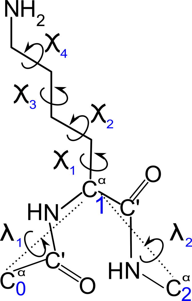
The potentials of mean force corresponding to the USC−corr contributions to the UNRES energy function were determined from the potential energy surfaces of terminally-blocked amino-acid residues, calculated in our previous work27,51 with the AM1 method of semiempirical quantum mechanics.52 The variables were the λ(1) and λ(2) dihedral angles, defined by Nishikawa et al.,53 for rotation of the first and the second peptide group, respectively, about the Cα ⋯ Cα virtual-bond axes and the χ(1), …, χ(m) dihedral angles for rotation of heavy atoms of side-chain, where m depends on the type of amino-acid residue (Figure 3). The grid sizes in all variables are summarized in Table 1.
Fig. 3.
Illustration of variables used for calculation of potential energy surfaces with the example of the lysine residue.
Table 1.
Grid sizes in λ(1), λ(2), the significant χ angles (involving rotation of non-hydrogen atoms), and the numbers of grid points for the 19 natural amino-acid residues with side chains (glycine is excluded, because it does not have a side chain). The amino-acid residues are grouped according to the number of significant χ angles.
| Grid size (degrees) | ||||||||||
|---|---|---|---|---|---|---|---|---|---|---|
| λ(1) | λ(2) | χ1 | χ2 | χ3 | χ4 | Residue(s) | ||||
| 0 | – | 30 | – | – | – | – | Pro | 12 | ||
| 30 | 30 | – | – | – | – | Ala, Gly | 144 | |||
| 1 | 30 | 30 | 30 | – | – | – | Cys, Ser, Thr, Val | 1728 | ||
| 2 | 30 | 30 | 30 | 30 | – | – | Asn, Asp, His, Ile, Leu, Phe, Trp, Tyr | 20736 | ||
| 3 | 30 | 30 | 30 | 30 | 60 | – | Glu, Gln, Met | 124416 | ||
| 4 | 30 | 30 | 30 | 60 | 120 | 120 | Arg, Lys | 93312 | ||
Number of significant χ angles.
Number of grid points.
The potentials of mean force were calculated from eq 3.
| (3) |
where is the potential of mean force, X and Y are the first and the second residue, respectively, H is the Hessian (second derivative of energy) matrix, e is the potential energy for a given conformation, m and n are the number of χ angles describing rotation of heavy atoms for residue X and Y, respectively.
The integration in backbone virtual-bond dihedral angles γ in eq 3 is carried out subject to the condition that a given value of the virtual-bond dihedral angle τ(k) has a given value. This angle depends on γ and the spherical angles α and β (Figure 1) of both side chains and, therefore, implicitly, on the side-chain angles . To carry out this part of the integration numerically, for each value of γ and for each orientation of both side-chain centroids, we computed the value of the respective angle τ(k) and added the Boltzmann factor (to the integrand in eq 3) to the bin in τ(k). The bin size was 30°. This value was a compromise between a discretization error of numerical integration, which should be as small as possible, and the fesibility of computing the potential-energy surfaces [it must be kept in mind that up to 4 side-chain dihedral angles χ are considered (Table 1)].
The presence of the γ − π − λ2 terms in eq 3 arises from the fact that λ2 is shared between residues X and Y in the dipeptide. The adiabatic energy surface, eX, of a terminally-blocked amino-acid residue X can be expressed as a function of the rotation of λ(1) and λ(2). The local angles of consecutive residues are related by eq 4:
| (4) |
The potentials for the virtual-bond-dihedral angles τ(1), τ(2), and τ(3) that involve side-chains were determined from potential energy surfaces and were subsequently fitted to the one-dimensional Fourier series (eq 5) by the linear least-squares method:
| (5) |
where X and Y are types of residues, amn, m = 1, 2, 3; n = 1, 2, … 4, bmn, m = 1, 2, 3; n = 1, 2, … 4 are coefficients of the Fourier expansions of .
2.3 Analysis of the USC−corr potentials
To determine how the USC−corr(τ(m)) potentials for pairs of amino-acid residues are similar to each other, for each type of potential, we computed the correlation coefficients of the potentials with the potential averaged over all residue types in the first and in the second position (X and Y), respectively. The correlation coefficients are defined by eq 6.
| (6) |
where is the potential profile averaged over residue types (X and Y), is the average value of this potential (averaged over τ(m)), and is the average value of a given potential (averaged over τ(m)). These quantities are defined by eqs 7, 8, and 9, respectively; it should be noted that the overline denotes averaging over residue types and the brackets 〈〉 denote averaging over τ(m).
| (7) |
where N(m) and M(m) are the numbers of residue types over which to sum for the respective type of the τ(m) angle: M(1) = 20, N(1) = 19; M(2) = 19, N(2) = 20; M(3) = N(3) = 19, because glycine does not have a side chain and is excluded from summation when the respective τ(m) angle depends on side-chain coordinates of residue X or Y, and {X(m)} and {Y (m)} are the sets of residue types over which to sum for a given type of τ angle.
| (8) |
| (9) |
A value of indicates that is correlated with (or, in other words, similar to) the average potential; more negative than −0.7 indicates anti-correlation (this means 50 % or more explained variance). Otherwise, the potential is not correlated or anti-correlated with the average potential.
2.4 Testing UNRES with the new potentials
The version of the UNRES force field optimized with the 1L2Y and 1LE1 proteins was used to test the newly derived and implemented physics-based USC−corr potentials. In contrast to the force-field used in our earlier work to test the statistical USC−corr potentials42 (which was optimized with 1GAB25), the force field optimized with 1LE1 and 1L2Y49 has no knowledge-based local-interaction potentials.
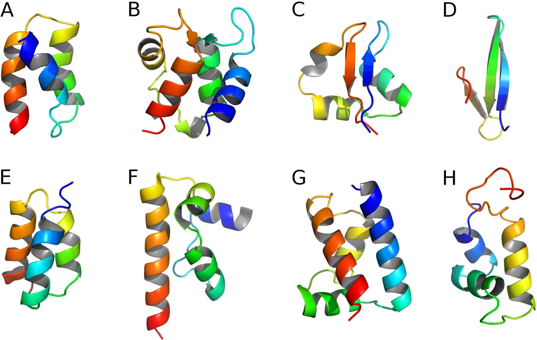
A set of small proteins (37–76 residues) used by us previously25,42 for assessing the performance of previous versions of the UNRES force field was selected as a training set. The set consisted of the recombinant B domain (FB) of staphylococcal protein A (PDB code: 1BDD)54 (α-helical structure), apo calbindin D9k from Bos taurus (PDB code: 1CLB)55 (α + β structure), the LysM domain from E. coli (PDB code: 1E0G)56 (α + β structure), the Fbp28 WW domain from Mus musculus (PDB code: 1E0L)57 (β structure), the GA module (PDB code: 1GAB)58 (α-helical structure), the DFF-C domain of DFF45/ICAD from Homo sapiens (PDB code: 1KOY)59 (α-helical structure), the POU-specific domain from Homo sapiens (PDB code: 1POU)60 (α-helical structure), and the purine repressor (PurR) DNA-binding domain from E. coli (PDB code: 1PRU61) (α-helical structure). Short N- and C-terminal fragments of the training proteins were truncated from the structures determined by NMR if the conformations of the NMR ensemble exhibited large fluctuations in these parts. The truncated experimental structures are shown in Figure 4. The training proteins exhibit low sequence similarity to each other; the highest sequence identity between the training proteins was 24.32%, as determined by the ClustalW2 program,62 with average identity of 9.69%.42
Fig. 4.
Cartoon representation of truncated experimental structures of training set proteins: A: 1BDD, B: 1CLB, C: 1E0G, D: 1E0L, E: 1GAB, F: 1KOY, G: 1POU, H: 1PRU. The chains are colored from blue (N-terminus) to red (C-terminus).
Subsequently, 22 proteins listed in Table 2 were selected to test the force field. The sizes of the selected proteins vary from 12 (for 1LE1) to 126 (for 1K40) amino-acid residues. Simulations were carried out for each protein of the set, using the force field with both the new terms and the best set of energy-term weights (wSC−corr = 0.25, wtor = i1.3431, wtord = 1.26571) and with the original force field.49
All simulations were run with the use of Multiplexed Replica Exchange Molecular Dynamics (MREMD).26,63,64 This procedure provides much better coverage of the conformational space compared to canonical molecular dynamics. For each tested protein with each weight set, 64 trajectories were run at 32 temperatures (2 trajectories per temperature). The temperatures ranged from 200 K to 500 K with a 10 K increment and, additionally, one pair of replicas was run at 295 K. Fifty million steps with length of 4.89 fs65 (0.24 µs total UNRES simulation time, which corresponds to about 0.24 ms because of UNRES time-scale extension resulting, in turn, from averaging out the fast degrees of freedom31,32) were run for every protein considered.
The Berendsen thermostat66 with the coupling parameter τ = 48.9 fs was used to maintain constant temperature. For each protein, the simulations were started from the extended structure. The variable time step (VTS) algorithm31 was used to integrate the equations of motion.
The energy-term weights applied in the calculations are collected in the first three columns of Table 3. The weights of the torsional (wtor) and double-torsional (wtord) terms were modified from the original values determined in ref 49 by subtracting a value ranging from wSC−corr to 3 × wSC−corr because the USC−corr potentials are likely to include some contributions from Utor and Utord. Reference runs with original values of wtor and wtord were also carried out.
Table 3.
Weights of the new USC−corr potentials, the torsional, and the double-torsional potentials and temperatures of heat capacity peaks [K] for 8 training proteins and all tested sets of energy-term weights.
| Energy-term weight | Temperatures [K] for proteins | ||||||||||
|---|---|---|---|---|---|---|---|---|---|---|---|
| wSC−corr | wtor | wtord | 1BDD | 1CLB | 1E0G | 1E0L | 1GAB | 1KOY | 1POU | 1PRU | Mean |
| 0.00 | 1.84316 | 1.26571 | 320 | 325 | 330 | 315 | 320 | 330 | 325 | 330 | 324.4 |
| 0.00 | 1.34316 | 1.26571 | 320 | 335 | 325 | 325 | 330 | 325 | 340 | 330 | 328.8 |
| 0.25 | 1.84316 | 1.26571 | 325 | 330 | 335 | 325 | 335 | 340 | 325 | 335 | 331.3 |
| 0.25 | 1.59316 | 1.26571 | 320 | 325 | 335 | 315 | 320 | 335 | 330 | 330 | 326.3 |
| 0.25 | 1.34316 | 1.26571 | 325 | 320 | 325 | 315 | 325 | 330 | 335 | 330 | 325.6 |
| 0.25 | 1.09316 | 1.26571 | 330 | 335 | 320 | 320 | 325 | 330 | 340 | 330 | 328.8 |
| 0.25 | 1.34316 | 1.01571 | 305 | 325 | 320 | 325 | 325 | 325 | 335 | 330 | 323.8 |
| 0.50 | 1.84316 | 1.26571 | 325 | 335 | 340 | 315 | 345 | 345 | 335 | 345 | 335.6 |
| 0.50 | 1.34316 | 1.26571 | 315 | 325 | 335 | 320 | 325 | 335 | 320 | 335 | 326.3 |
| 0.50 | 0.84316 | 1.26571 | 330 | 335 | 320 | 320 | 330 | 330 | 330 | 325 | 327.5 |
| 0.57 | 1.84316 | 1.26571 | 320 | 330 | 335 | 320 | 325 | 340 | 325 | 330 | 328.1 |
| 1.00 | 1.84316 | 1.26571 | 335 | 340 | 345 | 330 | 350 | 340 | 340 | 355 | 341.9 |
| 1.00 | 0.00000 | 1.26571 | 335 | 335 | 315 | 325 | 335 | 345 | 325 | 325 | 330.0 |
To standardize the analysis of the resulting structures and trajectories, the sets of conformations after performing WHAM analysis25,67 were always divided into five clusters by using different cut-off values in Ward’s minimum-variance method;68 this number of clusters is the same as the maximum number of models of a given target that a group can submit in the CASP experiments.
For each training protein, clustering was carried out in two ways. In the first approach, the temperature to calculate the statistical weights of the conformations was chosen ≈10 K below the heat capacity peaks (shown in Table 3), as in ref 25. However, for some of the calculations, the heat-capacity curves possessed multiple peaks and the statistical weights of conformations related to these peaks were calculated, and clustering was carried out at 210 K, 240 K, 270 K, 290 K and 310 K.
The Cα root-mean-square deviation (Cα RMSD) was used as a measure of the agreement between the calculated and the experimental structures. Because MREMD simulations produce conformational ensembles, mostly the ensemble-averaged RMSDs were used for analysis. The four analyzed RMSD values are defined by eqs 10 – 12, respectively.
| (10) |
| (11) |
| (12) |
where ρi is the Cα RMSD of the ith conformation, Ta is the absolute temperature and wk(Ta) is the weight of the kth conformation obtained in the MREMD simulations.
For each of the proteins of the test set, the lowest RMSD value from whole simulation (ρmin) and the average RMSD of the of the lowest-RMSD (the most native-like) cluster () at 290 K were determined.
3 Results and discussion
3.1 Analysis of the derived USC−corr potentials of mean force
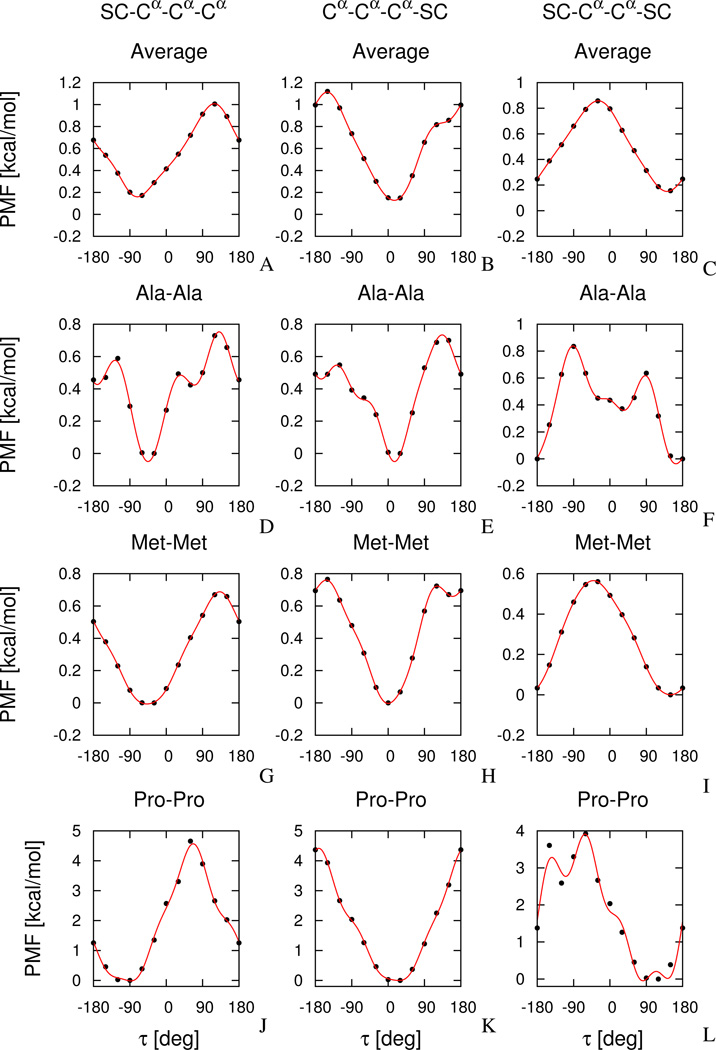
Plots of all 380 SC ⋯ Cα ⋯ Cα ⋯ Cα [], all 380 Cα ⋯ Cα ⋯ Cα ⋯ SC [], and all 361 SC ⋯ Cα ⋯ Cα ⋯ SC [] potentials are shown in Figure S1 of Supplementary Material. The plots of nine sample potentials (D–L) and of the three potentials (A–C) averaged over residue types (, m = 1, 2, 3; eq 7), are shown in Figure 5.
Fig. 5.
Plots of average side-chain-backbone potentials (A–C), [, m = 1, 2, 3; eq 7]; and sample side-chain backbone correlation potentials: UAlaAla(τ(m)), m = 1, 2, 3 (D–F), UMetMet(τ(m)), m = 1, 2, 3, (G–I), and UProPro(τ(m)), m = 1, 2, 3 (J–L). Black circles represent the values of the dimensionless PMFs calculated from histograms (eq 3) and red lines represent one-dimension Fourier series fits (eq 5) to the PMF values.
The average potentials (Figure 5A–C) are smooth and possess the global minimum at about τ(1) ≈ −60°, [for ], τ(2) ≈ 0° [for ], and τ(3) ≈ 150° [for ], respectively. The maxima are at τ(1) ≈ 120°, (for ), τ(2) ≈ −150° (for ), and τ(3) ≈ −30° (for ), respectively. The minima and maxima are thus separated by about 180°, which is understandable because one orientation corresponds to minimum steric repulsion of the peptide group linking the two central α-carbon atoms with the attached side chains and the other one to increased repulsion. Also, for this reason, the potentials are shifted with respect to each other; the shift angle reflects the phase-angle difference of the projection of a terminal Cα ⋯ Cα and Cα ⋯ SC virtual bond onto the plane perpendicular to the central Cα ⋯ Cα virtual bond. As can be seen from Figure 5A–C and 5G–I, the average potential is almost identical with the potential for methionine; as can be seen from Figure S1, this also holds for other bulky non-branched residues (e.g., Phe, Tyr, Trp, etc.). In contrast to this, as can be seen from Figure 5D–F and from Figure S1, small or branched residues such as, e.g., Ala, Val, and Leu have potentials that possess more fine structure. All these potentials, however, possess a similar free-energy span of about 1 kcal/mol. Proline (Figures 5J–L) is a special case and has a more pronounced energy span of about 5 kcal/mol. Another special case is glycine which does not have a side chain and has, therefore, potential patterns different from those of other residues (Figure S1). It should be noted that the potentials are undefined for this residue. The different conformational preferences of proline and glycine residues were also found in other theoretical and experimental studies.69,70
An inspection of the dominant conformations of the dipeptides corresponding to the global minima in the potentials (m = 1, 2, 3) shows that the backbone has an extended conformation and that hydrogen bonds between the carbonyl-oxygen atom of the preceding peptide group and the amide-hydrogen atom of the succeeding peptide group are formed at each residue (the C7 conformations), unless it is a proline. This is understandable because only the intra-residue energies are considered in eq 3. Thus, the specificity of the potentials lies in subtle details of the position of the minima and in differences in PMF barriers, depending on the kind of amino-acid side chains.
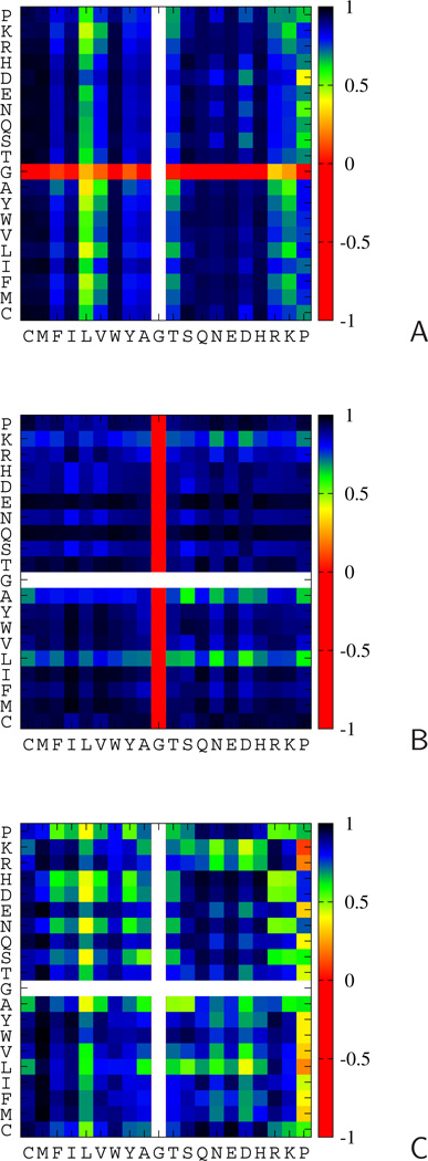
The correlation coefficients of the average potential with all other potentials, shown in Figure 6, confirm the above observations; for bulky residues such as cystine, methionine, phenylalanine, tryptophan, the correlation coefficients with the average potentials are high if the type of potential includes such a side chain [or two such side chains for the USC−corr(τ(3)) potentials]. The correlation with the average potential is weak for branched or small residues; additionally, it is weak for residues with oppositely charged side chains, because of hydrogen-bond formation (it should be noted that only uncharged side chains were considered when constructing energy maps).27 The UX−Gly(τ(1)) and UGly−X(τ(2)) potentials exhibit anti-correlation with the respective average potentials, which reflects the fact that glycine does not have a side chain. It can also be seen from Figure 6 that the side chain of the first residue has a greater influence on the potential than the side chain of the second residue. Therefore the and potentials are more sequence specific than the potentials. This feature is manifested in that the specific potentials (Figure 6B) are much more correlated with the average than the and potentials (Figure 6A and C). This result is consistent with the analysis for statistical potentials,42 for which the potentials showed greater correlation with the backbone torsional potentials than potentials for angles τ(1) and τ(3).
Fig. 6.
Color plots of the correlation coefficients of the respective potentials with the respective potentials averaged over all residue types at positions X and Y (eq 6). A: (for the Cα ⋯ Cα ⋯ Cα ⋯ SC angles, τ(1) B: (for the SC ⋯ Cα ⋯ Cα ⋯ Cα angles, τ(2)), C: (for the SC ⋯ Cα ⋯ Cα ⋯ SC angles, τ(3)). The color scales are on the right bars of each panel. Types of residues X are on the abscissae and types of residues Y are on the ordinates. The color scale is shown on the right side of each panel.
3.2 Performance of the new potentials in ab initio simulations of protein structure
To preliminary calibrate and test the performance of the new potentials, MREMD simulations were run on the training proteins for each set of wSC−corr, wtor, and wtord values summarized in the first three columns of Table 3. For each run, heat-capacity curves were calculated during the progress of simulations and monitored for convergence, as described in our earlier work.25,42,64,71 Simulations were terminated when the heat-capacity curves calculated from at least two consecutive time windows of a given simulation overlapped closely. Sample plots of heat-capacity curves during the progress of the MREMD run for 1E0L are shown in Figure 7.
Fig. 7.
Sample convergence plots of the heat capacity of 1E0L for wSC−corr = 0.0 (standard value), wtor = 1.84316 (standard value) and wtord = 1.26571 (standard value) (A), wSC−corr = 0.25, wtor = 1.84316 (standard value) and wtord = 1.26571 (standard value) (B), wSC−corr = 0.25, wtor = 1.34316 and wtord = 1.26571 (standard value) (C), and wSC−corr = 1.0, wtor = 0.0, wtord = 1.26571 (standard value) (D). Different colors denote heat-capacity curves for consecutive windows of the MREMD simulation, for the range from 10,000 to 50,000,000 MD steps divided into 8 equal windows. Windows are colored in order: red, orange, yellow, green, cyan, blue, purple, black.
We noticed that the convergence of the heat capacity curves was faster and the heat-capacity profiles were narrower with the new potentials (wSC−corr > 0) than without the new potentials (wSC−corr = 0) (compare Figure 7A and 7B). When the value of wtor was diminished by subtracting wSC−corr the convergence was even faster, but the heat-capacity profiles became wider (Figure 7C and 7D). Also, with increasing wSC−corr, the average temperature of the heat capacity peaks increased by up to 17.5 K, from 324.4 for wSC−corr = 0 to 341.9 for wSC−corr = 1 (Table 3) which is understandable, because UNRES with the new terms has not yet been optimized to reproduce the thermodynamic properties of proteins. This optimization is currently being carried out with the maximum-likelihood method.
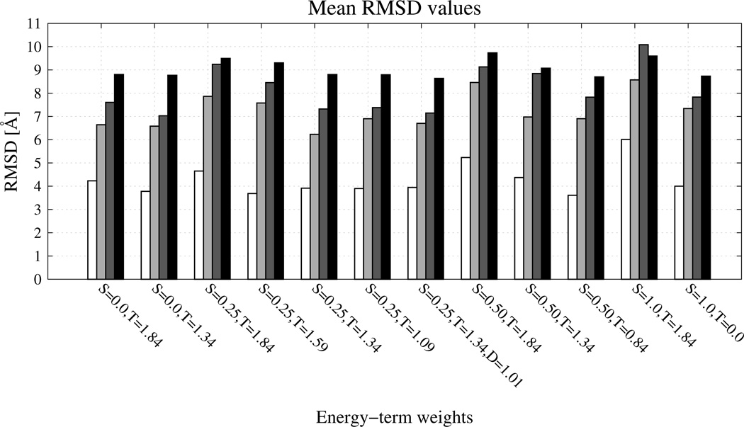
The values of ensemble-averaged RMSD (〈ρ〉(Ta)), of the RMSD averaged over the conformations of the lowest-RMSD cluster (), and the lowest RMSD found in a run (ρmin) averaged over all eight training proteins are shown in Figure 8 as bar diagrams. As can be seen from Figure 8, introducing the new physics-based USC−corr potentials without tuning other parameters resulted in higher values of RMSD, while RMSD decreased on average when the new potentials were introduced together with reducing wtor.
Fig. 8.
Bar diagrams of various RMSDs averaged over 8 proteins. White bars show the lowest RMSD obtained during the corresponding MREMD run [ρmin of eq 12], light-grey bars show the minimum of the cluster-averaged RMSD [ of eq 11] from five temperatures of clustering (210, 240, 270, 290 and 310 K), dark-grey bars show the minimum of the cluster-averaged RMSD [ of eq 11] from the temperature of clustering 10 K lower than the heat capacity peak, and the black bars show the RMSD averaged over the conformational ensemble generated during the MD run by WHAM in the last part of the simulation. S stands for wSC−corr, T stands for wtor, D stands for wtord.
The lowest values of ρmin averaged over all eight training proteins (white bars on Figure 8), were observed for wSC−corr = 0.50, wtor = 0.84316, wtord = 1.26571 (by 0.55 Å) and for wSC−corr = 0.25, wtor = 1.34316, wtord = 1.26571 (by 0.62 Å), respectively. Because the lowest-RMSD structures were obtained for the force fields in which the original wtor is reduced by subtracting twice the value of wSC−corr, it can be concluded that the USC−corr potentials include some information already encoded in the Utor potentials.
For averaged over all eight training proteins, a significant decrease (by 0.41 Å; light-grey bars in Figure 8) at T = 210 K, 240 K, 270 K, 290 K, and 310 K was observed for only one set of weights: wSC−corr = 0.25, wtor = 1.34316, wtord = 1.26571. However, for these weights, the (dark-grey bars on Figure 8) computed at a temperature 10 K lower than that of the maximum of the respective heat-capacity curve are higher than those computed at the five temperatures listed above; this feature probably results from the fact that the force field with the new potentials was not yet parameterized using thermodynamic data of proteins. At temperatures 10 K lower than those of the respective heat-capacity peaks, the simulations with the following three sets of parameters resulted in reduced values with respect to the force field without the new terms: for wSC−corr = 0.25, wtor = 1.34316, wtord = 1.01571 ( decreased by 0.46 Å), for wSC−corr = 0.25, wtor = 1.34316, wtord = 1.26571 ( decreased by 0.28 Å), and wSC−corr = 0.25, wtor = 1.09316, wtord = 1.26571 ( decreased by 0.23 Å).
As can be seen from Figure 8, the ensemble-averaged RMSD values (〈ρ〉(Ta)) did not change remarkably after implementing the new USC−corr potentials (black bars in Figure 8). Together with the observation regarding , this observation suggests that the new potentials do not result in improving the ability of UNRES to predict overall folds but improve the quality of those UNRES-predicted structures which have correct global fold. In summary, weighting the new terms with wSC−corr = 0.25, together with modifying the weights of the torsional and double-torsional terms (wtor = 1.34316 and wtord = 1.26571, respectively) consistently improves the quality of the calculated structures with respect to the the force field without the torsional terms.49
To assess the effect of reducing the torsional terms without introducing the new side-chain-torsional terms, control simulations were also run with wSC−corr = 0.0, wtor = 1.34316, wtord = 1.26571. As can be seen from Figure 8, only reduction of the torsional terms results in a lower average ; the other RMSDs increase by a small amount. Removing the new potentials with simultaneous reduction of wtor and wtord in particular results in deterioration of the quality of the calculated β-sheet segments, as can be seen from Figure 2S with the example of 1E0L protein (a β-structure protein).
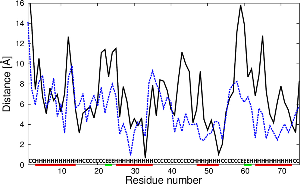
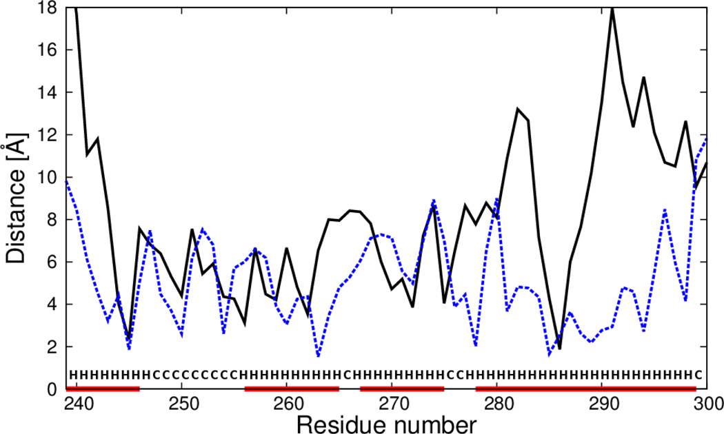
To determine what sections of the calculated structures were most improved by introducing the new terms, plots of the deviations of the Cα atoms of the mean structures corresponding to the most native-like clusters from those of the experimental structures, as functions of residue number in the sequence were constructed and analyzed. The deviations were calculated at optimal superposition of the computed structure on the experimental structure. As an example, the plots for 1CLB and 1KOY structures for which the most significant improvement was obtained (with wSC−corr = 0.25, wtor = 1.34316, wtord = 1.26571) are shown in Figure 9 and Figure 10, respectively. For 1CLB, the biggest improvement is observed for residues 20–25, 40–45 and 55–70, which covers the loop regions with small β-sheets, and for the C-terminal helix in the experimental structure. The calculated structure of 1KOY is improved mostly for residues 239–244, 264–268, 281–285 and 287–299, which cover the α-helical parts of the protein.
Fig. 9.
Plot of distances between Cα atoms of the average structures of the most native-like cluster of simulated 1CLB structures from the respective Cα atoms of the experimental 1CLB structure after optimal superposition. Solid black line: calculations with standard force field parameters (wSC−corr = 0.25, wtor = 1.34316, wtord = 1.26571),49 dashed black line: the force field that includes the , m = 1, 2, 3 potentials derived in this work (wSC−corr = 0.25, wtor = 1.34316, wtord = 1.26571). Red horizontal lines on the abscissa mark α-helices in the experimental structure.
Fig. 10.
Plot of distances between Cα atoms of the average structure of the most native-like cluster of simulated 1KOY structure from the respective Cα atoms of the experimental 1KOY structure after optimal superposition. Solid black line: calculations with standard force field parameters (wSC−corr = 0.25, wtor = 1.34316, wtord = 1.26571),49 dashed black line: the force field that includes the , m = 1, 2, 3 potentials derived in this work (wSC−corr = 0.25, wtor = 1.34316, wtord = 1.26571). Red horizontal lines on the abscissa mark α-helices in the experimental structure.
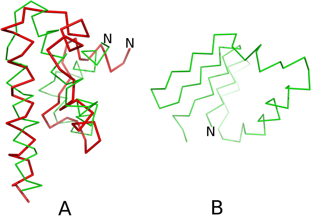
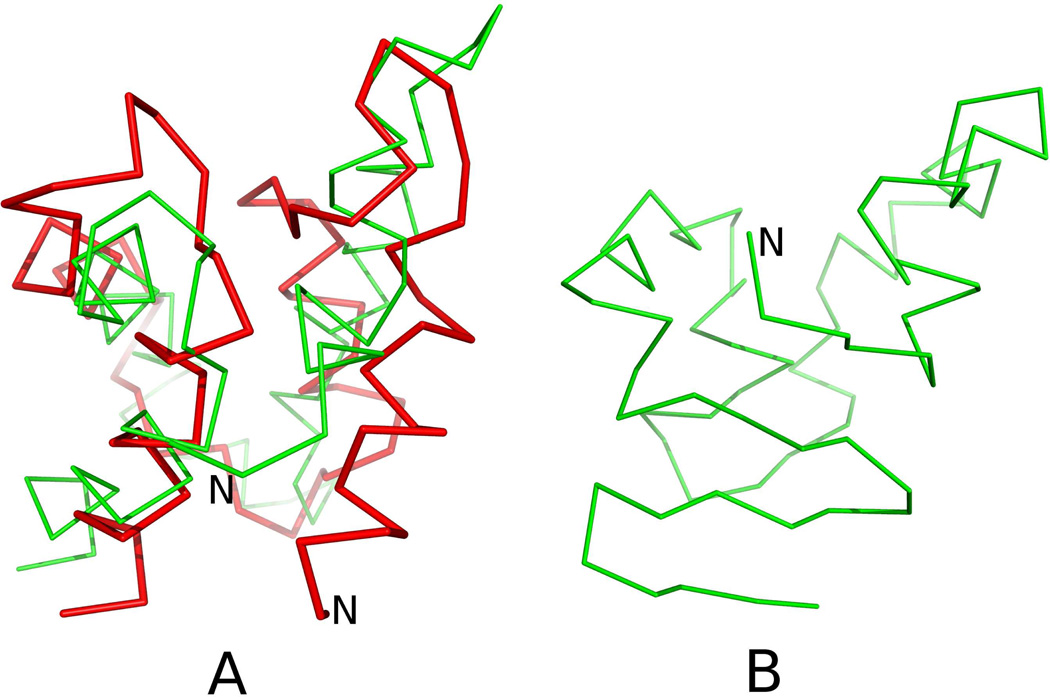
The structure of 1CLB calculated with the force field derived in ref 49 has an RMSD of 7.90 Å from the experimental structure. In the calculated structure, only the two middle α-helices are present, while the N- and the C-terminal α-helix are converted into β-sheets (Figure 11B). The structure predicted with new potentials (wSC−corr = 0.25, wtor = 1.34316, wtord = 1.26571) (Figure 11B) has RMSD of 6.04 Å and all α-helical parts are formed in that structure. The better agreement of that structure with the experimental 1CLB structure is even more evident when comparing the Global Distance Test (GDT TS) scores,72 for distance up to 4 Å which increased from 0.28 to 0.53, which means that the number of residues within 4 Å cutoff is greater by 89%. Both sets of parameters were unable to predict two small β-sheets correctly, which is the reason why α-helical parts with the new parameters are packed wrongly.
Fig. 11.
A: Superposition of the Cα-trace of the average structure of the most probable cluster of conformations of 1CLB obtained in MREMD simulations with inclusion of the potentials derived in this work (green lines) on that of the experimental structure of 1CLB (red lines). B: the average structure of the most probable cluster of conformations of 1CLB obtained in MREMD simulations with wSC−corr = 0.0, wtor = 1.84316, wtord = 1.26571 (without new potentials). The RMSDs from the experimental structures are 6.04 Å for panel A and 7.90 Å for panel B, respectively
A similar situation occurs for 1KOY. The structure calculated with the force field of ref 49 (without the new terms) forms the α+β-structure instead of α-helical structure (Figure 12B), with RMSD from the native structure equal to 9.23 Å. Conversely, simulations with new parameters (wSC−corr = 0.25, wtor = 1.34316, wtord = 1.26571) resulted in correct secondary structure with RMSD equal to 5.25 Å. Contrary to the previous work,42 in which implementation of statistical potentials results mainly in improvements of the loop regions, the physics-based version of the UNRES force field also contributes to correct recognition of regular secondary structure elements (α-helix and β-sheet).
Fig. 12.
A: Superposition of the Cα-trace of the average structure of the most probable cluster of conformations of 1KOY obtained in MREMD simulations with inclusion of the potentials derived in this work (green lines) on that of the experimental structure of 1KOY (red lines). B: the average structure of the most probable cluster of conformations of 1KOY obtained in MREMD simulations with wSC−corr = 0.0, wtor = 1.84316, wtord = 1.26571 (without new potentials). The RMSDs from the experimental structure are 5.25 Å for panel A, and 9.23 Å for panel B, respectively.
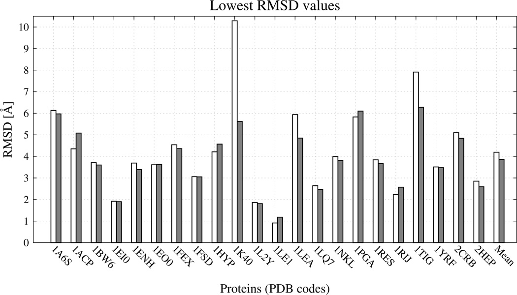
To test the performance of the force field, calculations were carried out for another set of 22 proteins, which were not utilized in the estimation of the weight of the new terms (see Table 2 for the list of these proteins). The calculations were run with the best set of energy-term weights (wSC−corr = 0.25, wtor = 1.34316, wtord = 1.26571) and, for reference, without the new potentials (wSC−corr = 0.0, wtor = 1.84316, wtord = 1.26571). The lowest RMSDs from the experimental structures are compared in Figure 13. The most significant decreases of ρmin with the new potentials (Figure 13) were observed for 1K40 (by 4.67 Å), 1TIG (by 1.63 Å) and 1LEA (by 1.09 Å), the average decrease of ρmin being 0.332 Å.
Fig. 13.
Bar diagrams of the lowest RMSDs from the experimental structures for 22 proteins from testing set. White bars: the lowest RMSD obtained in MREMD simulations [ρmin of eq 12] with the UNRES force field without new terms. Light-grey bars: ρmin with the best set of new terms.
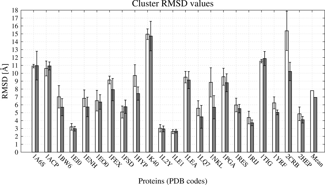
The RMSDs from the experimental structures corresponding to the mean structures of the most native-like clusters of the proteins studied are plotted, together with the respective error bars, in Figure 14. For each of the test proteins, the RMSD error was estimated by computing the standard deviation of the RMSD of the structures of the selected (most native-like) cluster from the RMSD of the mean structure of that cluster. It can be seen that noticeable improvement (over 1 Å) of (Figure 14) was observed for the following 8 out of 22 test proteins: 1BW6, 1ENH, 1FEX, 1HYP, 1LQ7, 1NKL, 1YRF, and 2CRB with average improvement of 0.86 Å. For none of tested proteins was a noticeable RMSD increase observed (beyond 0.67 Å).
Fig. 14.
Bar diagrams of the RMSDs of the mean structures of the most native-like clusters [ of eq 11] for the 22 test proteins corresponding to clustering at T = 290 K. White bars: the UNRES from force field without new terms. Light-grey bars: the UNRES force field with the new terms and optimal energy-term weights (wSC−corr = 0.25, wtor = 1.34316, wtord = 1.26571). For each protein and each force field, the error bar represents the standard deviations of the RMSDs of the structures of the most native-like cluster from the RMSD of the average structure of that cluster.
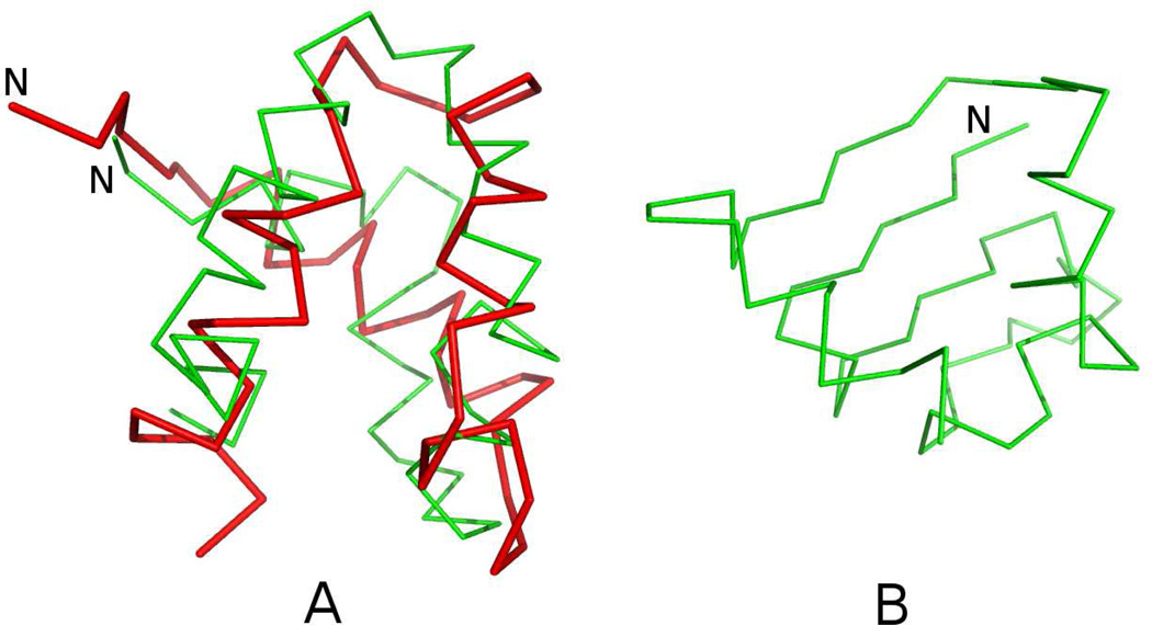
The biggest improvement in the reproduction of the experimental secondary structures was observed for 1FEX, for which the UNRES force field generated α+β-structures without the new terms instead of the native α-helical structure (Figure 15). These results, together with the results obtained with the training proteins, strongly suggests that that newly implemented physics-based potentials improve fold recognition.
Fig. 15.
A: Superposition of the Cα-trace of the average structure of the most probable cluster of conformations of 1FEX obtained in MREMD simulations with inclusion of the potentials derived in this work (green lines) on that of the experimental structure of 1FEX (red lines). B: the average structure of the most probable cluster of conformations of 1FEX obtained in MREMD simulations with wSC−corr = 0.0, wtor = 1.84316, wtord = 1.26571 (without new potentials). The RMSDs from the experimental structure are 7.93 Å for panel A, and 9.15 Å for panel B, respectively.
To test the capacity of the UNRES force field with the new potentials to reproduce the content of secondary structure in yet another way, as in our previous work,73 we computed the change of the free-energy of α-helical structure formation upon the replacement of x=Gly with a given amino-acid residue (ΔΔGhel). For this purpose, we used the KLALKLALxxLKLALKLA host-guest peptides studied experimentally by Krause and coworkers.74 The calculated values of ΔΔGhel are defined by eq 14.73
| (13) |
with
| (14) |
where R is the universal gas constant, T is the absolute temperature, and fhel(x) is the ensemble-averaged fraction of α-helical structures in the ensemble for the host-guest peptide containing a pair of specific residues x. The temperature T was set at 298 K, as in the experiment. A residue was considered to be in the α-helical state if the peptide group preceding it formed a hydrogen-bonding contact with the third succeeding peptide group; the presence of a hydrogen-bonding contact was assessed based on the mean-field energy of interactions, which depends on the distance between the centers of the two peptide groups; the details of this methods are described in ref 75.
The computed values of ΔΔGhel are compared with the experimental data from ref 74 in Table 4. It can be seen from Table 4 that the values computed with the new potentials are about 1.9 kcal/mol closer to the experimental values74 than those computed without the new potentials. This result suggests that the new potentials significantly improve the agreement of the thermodynamics of secondary-structure formation with the experiment.
Table 4.
The Gibbs free energy differences of α-helical structure formation in the KLALKLALxxLKLALKLA host-guest peptides with respect to glycine host-guest peptide
| Residue Name | ΔΔGhel;expa | ΔΔGhel;newb | ΔΔGhel;oldc | |ΔΔGhel;exp − ΔΔGhel;new| | |ΔΔGhel;exp − ΔΔGhel;old| |
|---|---|---|---|---|---|
| Pro | 6.64 | 0.81 | 0.48 | 5.83 | 0.33 |
| Lys | −0.66 | −0.51 | −3.33 | 0.15 | 2.82 |
| Arg | −1.33 | −0.56 | −3.48 | 0.77 | 2.92 |
| His | −2.23 | −0.35 | −3.55 | 1.88 | 3.2 |
| Asp | −2.12 | −1.7 | −3.49 | 0.42 | 1.79 |
| Glu | −1.12 | −0.59 | −3.48 | 0.53 | 2.89 |
| Asn | −1.44 | −0.48 | −3.36 | 0.96 | 2.88 |
| Gln | −0.59 | −0.58 | −3.5 | 0.01 | 2.92 |
| Ser | −1.43 | −0.04 | −3.31 | 1.39 | 3.27 |
| Thr | −2.16 | −0.43 | −3.65 | 1.73 | 3.22 |
| Ala | 0.18 | −0.06 | −3.3 | 0.24 | 3.24 |
| Tyr | 1.88 | −0.34 | −3.75 | 2.22 | 3.41 |
| Trp | −0.26 | 0.02 | −3.58 | 0.28 | 3.6 |
| Val | −2.24 | 0.09 | −3.61 | 2.33 | 3.7 |
| Leu | −0.23 | 0.44 | −3.61 | 0.67 | 4.05 |
| Ile | −0.89 | 0.24 | −4.01 | 1.13 | 4.25 |
| Phe | 1.72 | 0.23 | −3.84 | 1.49 | 4.07 |
| Cys | 0.58 | 0.23 | −1.5 | 0.35 | 1.73 |
| Met | 0.15 | 0.21 | −3.73 | 0.06 | 3.94 |
| Average | −0.29 | −0.18 | −3.24 | 1.18 | 3.06 |
4 Summary
The new sidechain–backbone correlation torsional potentials of mean force depending on the SC ⋯ Cα ⋯ Cα ⋯ Cα (τ(1)), Cα ⋯ Cα ⋯ Cα ⋯ SC (τ(2)), and SC ⋯ Cα ⋯ Cα ⋯ SC (τ(3)) angles (1121 potentials total) were derived from AM1 potential energy surfaces of terminally-blocked amino-acid residues calculated in our earlier work.27 By comparing the respective average potentials for each type of dihedral angle, the derived potentials were analyzed for similarity. Apart from obvious dissimilarity of the potentials involving the glycine and the proline residue, it was found that other residues can be grouped in three classes regarding the similarity of the potentials: bulky residues (e.g., cystine, methionine, phenylalanine, and tryptophan), and branched and small residues (e.g., leucine, alanine, serine, threonine), and charged residues. This division largely overlaps with the classification of residues proposed by Solis and Rackovsky,76 which was based on statistical analysis of physicochemical properties of amino-acid residues.
One-dimensional Fourier series were fitted to the obtained potentials, and the resulting formulas were implemented in the UNRES force field. The potentials were implemented in the UNRES force field package. It was found that introduction of the new potentials must be accompanied by reduction of the weight of the torsional terms to result in improvement of the calculated structures. On average the RMSD of the native-like clusters improved by 0.41 Å for the training set and by 0.86 Å for the test set of proteins, respectively. These results correspond to the best set of parameters: wSC−corr = 0.25, wtor = 1.34316, wtord = 1.26571. Work on complete optimization of the new potentials to take into account the structural and thermodynamic properties of proteins is now underway in our laboratory.
From Figure 13 it can be concluded that, after introducing the new terms, the lowest RMSD from the native structures is about 4 Å on average for the set of 22 proteins with which the modified force field was tested. This value is about 2 times larger than the average value of 2 Å for the set of 12 proteins studied by Lindorff-Larsen et al. by using the all-atom simulations with the all-atom force field (the modified CHARMM force field77) and the ANTON supercomputer.16 This difference might reflect the difference in the resolution of the coarse-grained and all-atom approaches. It should be noted, though, that the selection of the 12 proteins studied in reference 16 was made based on their foldability with the force field used, while the 22 proteins used in this study were not selected based on their foldability with UNRES. Therefore, it is also likely that the UNRES force field can still be improved by elaborating on the potentials of local interactions (as done in this work) and on force-field calibration. For example, for 1EI0 (38 residues) the lowest RMSD is below 2 Å and for 1LQ7 (67 residues) the lowest RMSD is below 3 Å.
The advantage of coarse-grained simulations over all-atom simulations is extension of the time scale and reduction of the cost of computations per MD step; both factors enable us to treat much larger systems at a much larger time scale than accessible to all-atom simulations. For example, the simulations of ref 16 were carried out for over 1000 µs to achieve folding, while the MREMD simulations of this work lasted only 0.25 µs UNRES time per trajectory (which amounts to about 250 µs real time per trajectory) and these simulations took from 4 to about 48 hours on a Beouwulf cluster, depending on protein size. Within this time, all simulations converged (Figure 7). This time-scale extension and reduction of computational cost enables us to run several tens or hundreds of trajectories even on a Beowulf cluster which, in turn, enables us to use parallel-tempering and related sampling techniques such as, e.g., MREMD to estimate ensemble averages and folding thermodynamics reliably or to run multiple-trajectories canonical simulations to determine folding kinetics such as, e.g., in our earlier study of protein A78 or in our recent study of the FBP 28 WW domain and its mutants.79 Extension of the time and size scale also enables us to treat biologically important processes such as, e.g., the opening of a Hsp70 chaperone recently studied by us with the used of molecular dynamics with UNRES.80
Supplementary Material
Acknowledgments
This work was supported by grant MPD/2010/5 and START scholarship (100.2014) from the Foundation for Polish Science (FNP), grant DEC-2011/01/N/ST4/01772 from the National Science Center of Poland, by grants from the National Institutes of Health (GM-14312) and the National Science Foundation (MCB10-19767). This research was supported by an allocation of advanced computing resources provided by the National Science Foundation (http://www.nics.tennessee.edu/), and by the National Science Foundation through TeraGrid resources provided by the Pittsburgh Supercomputing Center. Computational resources were also provided by (a) the supercomputer resources at the Informatics Center of the Metropolitan Academic Network (IC MAN) in Gdańsk, (b) the 792-processor Beowulf cluster at the Baker Laboratory of Chemistry, Cornell University, and (c) our 184-processor Beowulf cluster at the Faculty of Chemistry, University of Gdańsk.
Footnotes
Description of the Supporting Information
Figure S1 presents plots of the PMFs for all side-chain backbone correlation potentials . Figure S2 presents bar diagrams for each of eight proteins from training set. This information is available free of charge via the Internet at http://pubs.acs.org
References
- 1.Duan Y, Kollman PA. Science. 1998;282:740–744. doi: 10.1126/science.282.5389.740. [DOI] [PubMed] [Google Scholar]
- 2.Sieradzan AK, Liwo A, Hansmann UHE. J. Chem. Theory Comput. 2012;8:3416–3422. doi: 10.1021/ct300528r. [DOI] [PMC free article] [PubMed] [Google Scholar]
- 3.Beckstein O, Sansom MSP. Phys. Biol. 2006;3:147. doi: 10.1088/1478-3975/3/2/007. [DOI] [PubMed] [Google Scholar]
- 4.Huo S, Wang J, Cieplak P, Kollman PA, Kuntz ID. J. Med. Chem. 2002;45:1412–1419. doi: 10.1021/jm010338j. PMID: 11906282. [DOI] [PubMed] [Google Scholar]
- 5.Feller SE, Pastor RE. J. Chem. Phys. 1999;111:1281. [Google Scholar]
- 6.Spackova M, Cheatham T, Ryjacek F, Lankas F, Van Meervelt L, Hobza P, Sponer J. J. Am. Chem. Soc. 2003;125:1759–1769. doi: 10.1021/ja025660d. PMID: 12580601. [DOI] [PubMed] [Google Scholar]
- 7.Zhao G, Perilla JR, Yufenyuy EL, Meng X, Chen B, Ning J, Ahn J, Gronenborn AM, Schulten K, Aiken C, et al. Nature. 2013;497:643–646. doi: 10.1038/nature12162. [DOI] [PMC free article] [PubMed] [Google Scholar]
- 8.Terstappen GC, Reggiani A. Trends Pharmacol. Sci. 2001;22:23–26. doi: 10.1016/s0165-6147(00)01584-4. [DOI] [PubMed] [Google Scholar]
- 9.Srinivasa Rao V, Srinivas K. J. Bioinform. Seq. Anal. 2011;3:89–94. [Google Scholar]
- 10.Pande VS, Baker I, Chapman J, Elmer S, Kaliq S, Larson SM, Rhee YM, Shirts MR, Snow CD, Sorin EJ, Zagrovic B. Biopolymers. 2003;68:91–109. doi: 10.1002/bip.10219. [DOI] [PubMed] [Google Scholar]
- 11.Hess B, Kutzner C, van der Spoel D, Lindahl E. J. Chem. Theory Comput. 2008;4:435–447. doi: 10.1021/ct700301q. [DOI] [PubMed] [Google Scholar]
- 12.Phillips JC, Braun R, Wang W, Gumbart J, Tajkhorshid E, Villa E, Chipot C, Skeel RD, Kalé L, Schulten K. J. Comput. Chem. 2005;26:1781–1802. doi: 10.1002/jcc.20289. [DOI] [PMC free article] [PubMed] [Google Scholar]
- 13.Bowers KJ, Chow E, Xu H, Dror RO, Eastwood MP, Gregersen BA, Klepeis JL, Kolossvary I, Moraes MA, Sacerdoti FD, Salmon JK, Shan Y, E.Shaw D. ACM/IEEE SC 2006 Conference (SC.06); 2006. pp. 43–43. [Google Scholar]
- 14.Friedrichs MS, Eastman P, Vaidyanathan V, Houston M, Legrand S, Beberg AL, Ensign DL, Bruns CM, Pande VS. J. Comput. Chem. 2009;30:864–872. doi: 10.1002/jcc.21209. [DOI] [PMC free article] [PubMed] [Google Scholar]
- 15.Shaw DE, et al. Commun. ACM. 2008;51:91–97. [Google Scholar]
- 16.Lindorff-Larsen K, Piana S, Dror RO, Shaw DE. Science. 2011;334:517–520. doi: 10.1126/science.1208351. [DOI] [PubMed] [Google Scholar]
- 17.Lindorff-Larsen K, Trbovic N, Maragakis P, Piana S, Shaw DE. J. Am. Chem. Soc. 2012;134:3787–3791. doi: 10.1021/ja209931w. [DOI] [PubMed] [Google Scholar]
- 18.Sanbonmatsu KY, Joseph S, Tung C-S. Proc. Natl. Acad. Sci. U. S. A. 2005;102:15854–15859. doi: 10.1073/pnas.0503456102. [DOI] [PMC free article] [PubMed] [Google Scholar]
- 19.Piana S, Lindorff-Larsen K, Shaw DE. Proc. Natl. Acad. Sci. U. S. A. 2012;109:17845–17850. doi: 10.1073/pnas.1201811109. [DOI] [PMC free article] [PubMed] [Google Scholar]
- 20.Piana S, Lindorff-Larsen K, Shaw DE. J. Phys. Chem. B. 2013;117:12935–12942. doi: 10.1021/jp4020993. [DOI] [PubMed] [Google Scholar]
- 21.Piana S, Klepeis JL, Shaw DE. Curr. Opinion Struct. Biol. 2014;24:98–105. doi: 10.1016/j.sbi.2013.12.006. [DOI] [PubMed] [Google Scholar]
- 22.Liwo A, Pincus MR, Wawak RJ, Rackovsky S, Scheraga HA. Protein Sci. 1993;2:1715–1731. doi: 10.1002/pro.5560021016. [DOI] [PMC free article] [PubMed] [Google Scholar]
- 23.Liwo A, Ołdziej S, Pincus MR, Wawak RJ, Rackovsky S, Scheraga HA. J. Comput. Chem. 1997;18:849–873. [Google Scholar]
- 24.Liwo A, Czaplewski C, Pillardy J, Scheraga HA. J. Chem. Phys. 2001;115:2323–2347. [Google Scholar]
- 25.Liwo A, Khalili M, Czaplewski C, Kalinowski S, Ołdziej S, Wachucik K, Scheraga H. J. Phys. Chem. B. 2007;111:260–285. doi: 10.1021/jp065380a. [DOI] [PMC free article] [PubMed] [Google Scholar]
- 26.Liwo A, Czaplewski C, Ołdziej S, Rojas AV, Kaźmierkiewicz R, Makowski M, Murarka RK, Scheraga HA. In: Coarse-Graining of Condensed Phase and Biomolecular Systems. Voth G, editor. Vol. 8. CRC Press; 2008. pp. 1391–1411. [Google Scholar]
- 27.Kozłowska U, Maisuradze GG, Liwo A, Scheraga HA. J. Comput. Chem. 2010;31:1154–1167. doi: 10.1002/jcc.21402. [DOI] [PMC free article] [PubMed] [Google Scholar]
- 28.Makowski M, Liwo A, Sobolewski E, Scheraga HA. J. Phys. Chem. B. 2011;115:6119–6129. doi: 10.1021/jp111258p. [DOI] [PMC free article] [PubMed] [Google Scholar]
- 29.Makowski M, Liwo A, Scheraga HA. J. Phys. Chem. B. 2011;115:6130–6137. doi: 10.1021/jp111259e. [DOI] [PMC free article] [PubMed] [Google Scholar]
- 30.Sieradzan AK, Scheraga HA, Liwo A. J. Chem. Theory Comput. 2012;8:1334–1343. doi: 10.1021/ct2008439. [DOI] [PMC free article] [PubMed] [Google Scholar]
- 31.Khalili M, Liwo A, Jagielska A, Scheraga H. J. Phys. Chem. B. 2005;109:13798–13810. doi: 10.1021/jp058007w. [DOI] [PMC free article] [PubMed] [Google Scholar]
- 32.Liwo A, Khalili M, Scheraga HA. Proc. Natl. Acad. Sci. U.S.A. 2005;102:2362–2367. doi: 10.1073/pnas.0408885102. [DOI] [PMC free article] [PubMed] [Google Scholar]
- 33.Liwo A, Lee J, Ripoll DR, Pillardy J, Scheraga HA. Proc. Natl. Acad. Sci., U. S. A. 1999;96:5482–5485. doi: 10.1073/pnas.96.10.5482. [DOI] [PMC free article] [PubMed] [Google Scholar]
- 34.Lee J, Scheraga HA. Int. J. Quant. Chem. 1999;75:255–265. [Google Scholar]
- 35.Ołdziej S, et al. Proc. Natl. Acad. Sci. U.S.A. 2005;102:7547–7552. doi: 10.1073/pnas.0502655102. [DOI] [PMC free article] [PubMed] [Google Scholar]
- 36.Liwo A, He Y, Scheraga HA. Phys. Chem. Chem. Phys. 2011;13:16890–16901. doi: 10.1039/c1cp20752k. [DOI] [PMC free article] [PubMed] [Google Scholar]
- 37.He Y, Mozolewska MA, Krupa P, Sieradzan AK, Wirecki TK, Liwo A, Kach-lishvili K, Rackovsky S, Jagieła D, Slusarz R, Czaplewski CR, Ołdziej S, Scheraga HA. Proc. Natl. Acad. Sci. U. S. A. 2013;110:14936–14941. doi: 10.1073/pnas.1313316110. [DOI] [PMC free article] [PubMed] [Google Scholar]
- 38.Gay JG, Berne BJ. J. Chem. Phys. 1981;74:3316–3319. [Google Scholar]
- 39.Kubo R. J. Phys. Soc. Japan. 1962;17:1100–1120. [Google Scholar]
- 40.Wu J, Zhen X, Shen H, Li G, Ren P. J. Chem. Phys. 2011;135:155104. doi: 10.1063/1.3651626. [DOI] [PMC free article] [PubMed] [Google Scholar]
- 41.Shen H, Li Y, Ren P, Zhang D, Li G. J. Chem. Theory Comput. 2014;10:731–750. doi: 10.1021/ct400974z. [DOI] [PMC free article] [PubMed] [Google Scholar]
- 42.Krupa P, Sieradzan AK, Rackovsky S, Baranowski M, Odziej S, Scheraga HA, Liwo A, Czaplewski C. J. Chem. Theory Comput. 2013;9:4620–4632. doi: 10.1021/ct4004977. [DOI] [PMC free article] [PubMed] [Google Scholar]
- 43.Bernstein FC, Koetzle TF, Williams GJB, Meyer EFJ, Brice MD, Rodgers JR, Kennard O, Shimanouchi T, Tasumi M. J. Mol. Biol. 1977;112:535–542. doi: 10.1016/s0022-2836(77)80200-3. [DOI] [PubMed] [Google Scholar]
- 44.Shen H, Liwo A, Scheraga HA. J. Phys. Chem. B. 2009;113:8738–8744. doi: 10.1021/jp901788q. [DOI] [PMC free article] [PubMed] [Google Scholar]
- 45.Kolinski A, Skolnick J. J. Chem. Phys. 1992;97:9412–9426. [Google Scholar]
- 46.Liwo A, Kaźmierkiewicz R, Czaplewski C, Groth M, Ołdziej S, Wawak RJ, Rackovsky S, Pincus MR, Scheraga HA. J. Comput. Chem. 1998;19:259–276. [Google Scholar]
- 47.Chinchio M, Czaplewski C, Liwo A, Ołdziej S, Scheraga HA. J. Chem. Theory and Comput. 2007;3:1236–1248. doi: 10.1021/ct7000842. [DOI] [PubMed] [Google Scholar]
- 48.Ołdziej S, Kozłowska U, Liwo A, Scheraga HA. J. Phys. Chem. A. 2003;107:8035–8046. [Google Scholar]
- 49.He Y, Xiao Y, Liwo A, Scheraga HA. J. Comput. Chem. 2009;30:2127–2135. doi: 10.1002/jcc.21215. [DOI] [PMC free article] [PubMed] [Google Scholar]
- 50.Neidigh JW, Fesinmeyer RM, Andersen NH. Nat. Struct. Biol. 2002;9:425–430. doi: 10.1038/nsb798. [DOI] [PubMed] [Google Scholar]
- 51.Kozłowska U, Liwo A, Scheraga HA. J. Comput. Chem. 2010;31:1143–1153. doi: 10.1002/jcc.21399. [DOI] [PMC free article] [PubMed] [Google Scholar]
- 52.Stewart JJ. J. Comput.-Aided Molec. Design. 1990;4:1–105. doi: 10.1007/BF00128336. [DOI] [PubMed] [Google Scholar]
- 53.Nishikawa K, Momany FA, Scheraga HA. Macromolecules. 1974;7:797–806. doi: 10.1021/ma60042a020. [DOI] [PubMed] [Google Scholar]
- 54.Gouda H, Torigoe H, Saito A, Sato M, Arata Y, Shimada I. Biochemistry. 1992;31:9665–9672. doi: 10.1021/bi00155a020. [DOI] [PubMed] [Google Scholar]
- 55.Skelton NJ, Krdel J, Chazin WJ. J. Mol. Biol. 1995;249:441–462. doi: 10.1006/jmbi.1995.0308. [DOI] [PubMed] [Google Scholar]
- 56.Bateman A, Bycroft M. J. Mol. Biol. 2000;299:1113–1119. doi: 10.1006/jmbi.2000.3778. [DOI] [PubMed] [Google Scholar]
- 57.Macias MJ, Gervais V, Civera C, Oschkinat H. Nat. Struct. Biol. 2000;7:375–379. doi: 10.1038/75144. [DOI] [PubMed] [Google Scholar]
- 58.Johansson MU, de Chateau M, Wikstrom M, Forsen S, Drakenberg T, Bjorck L. J. Mol. Biol. 1997;266:859–865. doi: 10.1006/jmbi.1996.0856. [DOI] [PubMed] [Google Scholar]
- 59.Fukushima K, Kikuchi J, Koshiba S, Kigawa T, Kuroda Y, Yokoyama S. J. Mol. Biol. 2002;321:317–327. doi: 10.1016/s0022-2836(02)00588-0. [DOI] [PubMed] [Google Scholar]
- 60.Assa-Munt N, Mortishire-Smith RJ, Aurora R, Herr W, Wright PE. Cell. 1993;73:193–205. doi: 10.1016/0092-8674(93)90171-l. [DOI] [PubMed] [Google Scholar]
- 61.Nagadoi A, Morikawa S, Nakamura H, Enari M, Kobayashi K, Yamamoto H, Sampei G, Mizobuchi K, Schumacher MA, Brennan RG. Structure. 1995;3:1217–1224. doi: 10.1016/s0969-2126(01)00257-x. [DOI] [PubMed] [Google Scholar]
- 62.Larkin M, Blackshields G, Brown N, Chenna R, McGettigan P, McWilliam H, Valentin F, Wallace I, Wilm A, Lopez R, Thompson J, Gibson T, Higgins D. Bioinformatics. 2007;23:2947–2948. doi: 10.1093/bioinformatics/btm404. [DOI] [PubMed] [Google Scholar]
- 63.Rhee YM, Pande VS. Biophys. J. 2003;84:775–786. doi: 10.1016/S0006-3495(03)74897-8. [DOI] [PMC free article] [PubMed] [Google Scholar]
- 64.Czaplewski C, Kalinowski S, Liwo A, Scheraga HA. J. Chem. Theory Comput. 2009;5:627–640. doi: 10.1021/ct800397z. [DOI] [PMC free article] [PubMed] [Google Scholar]
- 65.Khalili M, Liwo A, Rakowski F, Grochowski P, Scheraga H. J. Phys. Chem. B. 2005;109:13785–13797. doi: 10.1021/jp058008o. [DOI] [PMC free article] [PubMed] [Google Scholar]
- 66.Berendsen HJC, Postma JPM, van Gunsteren WF, DiNola A, Haak JR. J. Chem. Phys. 1984;81:3684–3690. [Google Scholar]
- 67.Kumar S, Bouzida D, Swendsen RH, Kollman PA, Rosenberg JM. J. Comput. Chem. 1992;13:1011–1021. [Google Scholar]
- 68.Späth H. Cluster Analysis Algorithms. New York: Halsted Press; 1980. [Google Scholar]
- 69.Hermans J. Proc. Natl. Acad. Sci. USA. 2011;108:3095–3096. doi: 10.1073/pnas.1019470108. [DOI] [PMC free article] [PubMed] [Google Scholar]
- 70.Grdadolnik J, Mohacek-Grosev V, Baldwin RL, Avbelj F. Proc. Natl. Acad. Sci. USA. 2011;108:1794–1798. doi: 10.1073/pnas.1017317108. [DOI] [PMC free article] [PubMed] [Google Scholar]
- 71.Nanias M, Czaplewski C, Scheraga HA. J. Chem. Theory Comput. 2006;2:513–528. doi: 10.1021/ct050253o. [DOI] [PMC free article] [PubMed] [Google Scholar]
- 72.Zemla A, Venclovas C, Moult J, Fidelis K. Proteins: Struct. Func. Genet. 2001;45(S5):13–21. doi: 10.1002/prot.10052. [DOI] [PubMed] [Google Scholar]
- 73.Sieradzan AK, Niadzvedtski A, Scheraga HA, Liwo A. J. Chem. Theory Comput. 2014;10:2194–2203. doi: 10.1021/ct500119r. [DOI] [PMC free article] [PubMed] [Google Scholar]
- 74.Krause E, Bienert M, Schmieder P, Wenschuh H. J. Am. Chem. Soc. 2000;122:4865–4870. [Google Scholar]
- 75.Ołdziej S, Liwo A, Czaplewski C, Pillardy J, Scheraga HA. J. Phys. Chem. B. 2004;108:16934–16949. [Google Scholar]
- 76.Solis AD, Rackovsky S. Proteins: Struct. Funct. Bioinf. 2000;38:149–164. [PubMed] [Google Scholar]
- 77.Brooks BR, et al. J. Comp. Chem. 2009;30:1545–1615. [Google Scholar]
- 78.Khalili M, Liwo A, Scheraga HA. J. Mol. Biol. 2006;355:536–547. doi: 10.1016/j.jmb.2005.10.056. [DOI] [PubMed] [Google Scholar]
- 79.Zhou R, Maisuradze GG, Sunol D, Todorovski T, Macias MJ, Xiao Y, Scheraga HA, Czaplewski C, Liwo A. Proc. Natl. Acad. Sci. U.S.A. 2014 doi: 10.1073/pnas.1420914111. submitted. [DOI] [PMC free article] [PubMed] [Google Scholar]
- 80.Golas EI, Maisuradze GG, Senet P, Ołdziej S, Czaplewski C, Scheraga HA, Liwo A. J. Chem. Theory Comput. 2012;8:1750–1764. doi: 10.1021/ct200680g. [DOI] [PMC free article] [PubMed] [Google Scholar]
Associated Data
This section collects any data citations, data availability statements, or supplementary materials included in this article.


