

Abstract
Ion Mobility Spectrometry (IMS) is a widely used and ‘well-known’ technique of ion separation in gaseous phase based on the differences of ion mobilities under an electric field. This technique has received increased interest over the last several decades as evidenced by the pace and advances of new IMS devices available. In this review we explore the hyphenated techniques that are used with IMS, especially mass spectrometry as identification approach and multi-capillary column as pre-separation approach. Also, we will pay special attention to the key figures of merit of the ion mobility spectrum and how data is treated, and the influences of the experimental parameters in both a conventional drift time IMS (DTIMS) and a miniaturized IMS also known as high Field Asymmetric IMS (FAIMS) in the planar configuration. The current review article is preceded by a companion review article which details the current instrumentation and to the sections that configures both a conventional DTIMS and FAIMS devices. Those reviews will give the reader an insightful view of the main characteristics and aspects of the IMS technique.
1. Hyphenated Methods
Ion Mobility Spectrometry (IMS) is an analytical technique based on ion separation in gaseous phase due to different ion mobilities under an electric field based on their size, mass and shape. Drift-time ion mobility spectrometers (DTIMS) are composed by four main parts1, 2: (1) Ionization Region, where samples are ionized; (2) Ion Gate, used to decide when the ions pass to the drift region; (3) Drift Region, where ions are separated due to their mobility; and (4) Detection Region, where ions are collected. Up to nine different designs of IMS have been reported3. The mainly used miniaturized version is the high Field Asymmetric Ion Mobility Spectrometry (FAIMS)1, 4. Ion filtering is achieved using a high asymmetric electric field (ideally with a rectangular shape) and scanned with a low DC field or compensation voltage (CV) that will allow, or not, the passage of ions with different mobilities. Over the past several decades, Ion Mobility Spectrometry has evolved into an inexpensive and powerful analytical technique for the detection of gas phase samples in the lower ng·L−1 (ppbv) levels at ambient pressures and temperatures5.
The IMS instrumentation has a wide range of applications3 from chemical weapons monitoring to biological and clinical analysis. In recent years, there has been an increase of new applications for complex samples, particularly for medicine (diagnosis, therapy and medication control e.g. for measuring metabolites in breath analysis)6–11, and for biological samples (cells, fungi, bacteria)12–20. For the analysis of these complex mixtures, ion mobility alone will likely not be sufficient for the identification of each analyte. Several analytes in these biological mixtures frequently have similar or even the same mobility. Real samples give complex IMS spectra, and identification of analytes can be difficult. Therefore, hyphenated techniques are used to improve the analysis of real samples.
Two hyphenated technique strategies are used: (1) Confirm ion identities using the IMS techniques as a pre-filter for mass spectrometry (MS) system21–26. Those systems are named IM-MS (ion mobility – mass spectrometry); (2) Pre-Separate the sample to reduce the cross-linked detection, as the sample compounds achieve the IMS at different times. This strategy is used for both gases and liquids. Pre-separation in the gas-phase has been used with gas chromatography (GC) and also with multi-capillary columns (MCC).
Gas chromatography (GC) with either conventional drift time IMS27 or FAIMS28. Coupling micro-fabricated planar FAIMS also known as Differential Mobility Spectrometry (DMS), to a GC results in multidimensional separations that rely both on chromatographic retention times and also on differential mobility K (inversely proportional to the compensation voltage CV) and the dispersion voltage (DV), providing a highly sensitive and selective analytical tool29–32. On the other hand, multi-capillary columns (MCC) which have successfully been used in combination with conventional drift time IMS for analysis of biological and medical samples7, 33–35. Furthermore, this avoids negative effects from clustering in the ionization chamber when humid air is analysed9, 36.
Pre-separation in the liquid-phase, has been used with liquid chromatography (LC) prior to an MS detection which can routinely yield thousands of protein identifications from a single sample37. The incorporation of an IMS drift cell between the LC separation and MS38, 39 has multiple advantages for analysing complex mixtures such as high speed measurements that allow multiple IMS–MS analyses across a given LC peak, a degree of orthogonality to both LC and MS analyses thereby increasing the overall peak capacity40, 41, and a highly reproducible drift time dimension.
Pre-separation will relate each analyte to two parameters, a specific ion mobility value (or drift time) and the time it takes to elute out from the pre-separation column (or retention time). This value is very characteristic of the particular analyte at a specific temperature, pressure, column length, polarity and flow rate. Providing these two values for relevant analytes in every analysis enables the identification of compounds in an unknown sample.
1.1 Mass Spectrometer as a Detector, the IM-MS
Mass spectrometry (MS) is a highly established field of chemical analysis and analytical science42, in which it measures the mass-to-charge ratio (m/z) of a molecular ion, an inherited property of molecule defined by the mass number m of an ion divided by its charge number z. A typical mass spectrum is represented by a plot of ion abundance (Y-axis) vs. increasing m/z units (X-axis in Daltons, Da). The X-axis of the mass spectrum are represented in terms of increasing m/z units), this m/z value can be directly correlated with the molecular weight of compounds of interest. Ion Mobility Spectrometry (IMS) separates ions based on size-to-charge ratios and Mass spectrometry (MS) detects ions based on their mass-to-charge (m/z) ratios. In IM-MS instrumentation, ions are separated on the size-to-charge ratio in the IMS component and the mass-to-charge ratio in the MS component. A two-dimensional separation is obtained based on size and mass43. The main advantage of coupling IM-MS is that IMS can separate isomers of the same chemical compound and MS identifies those compounds.
The set of IM-MS instruments provide unambiguous identification of ions in a mobility spectrum and was first described in 196244 and were commercially available since the 1970s but it was mainly used for aqueous and solid samples like proteins, lipids, or alcohols and not for VOC applications43, 45, 46. Nowadays, there has been an expansion in new applications for biomolecules for detecting peptides47, lipids48, oligosaccharides49 and even virus50. Some excellent overviews about different coupling technologies of IMS with MS have been given recently43, 51, 52. Also FAIMS-MS instruments are available53, 54. An outlet at the end of the drift tube provides a path to the MS system, with pumps along the path to lower the pressure of the ion-carrying gas prior to injection. Also, ion transmission has been improved by implementing an electrodynamic ion funnel for their re-focusing into tight circular beams at the FAIMS-MS interface55–57.
In MS the chemical information acquired are derived from gas phase ions, in Figure 1 is shown a simplified diagram of the detector operation. As the analytes are eluted from the analytical column, it is then ionized to induce a charge and introduced into the mass analyser, where the ions are detected. The signal is then amplified via an electron multiplier. Data analysis and mass spectral interpretations are processed by a specialized software package resulting in a plot of ion abundance vs. increasing m/z unit. Usually, the mass spectra is de-convolution and the peaks are identified using databases like NIST58 other Wiley59.
Figure 1.

Basic components of a typical mass spectrometer. *FT-ICR does not use an electron multiplier. APCI, atmospheric-pressure chemical ionization; ESI, electrospray ionization; MALDI, matrix-assisted laser desorption/ionization; FT-ICR, Fourier transform ion-cyclotron resonance. Reprinted with permission from Ref. 42. Copyright (2003) Nature Publishing Group.
The different types of mass analysers measure ions in different ways. In most analytical measurements, two of the predominant figures of merit are accuracy and precision. It is important to note that an accurate measurement does not necessarily require a precise measurement and vice versa. In MS42, the precision of the measurement is related to the resolution (that is, the ability to resolve two adjacent peaks). In general, resolution is defined as m/Δm, where m is the integer mass of the peaks being resolved and Δm is the mass difference between the two peaks.
IM-MS is a powerful analytical technique that combines the benefits traditionally associated with MS, such as high sensitivity and mass accuracy, with the ability to distinguish ions with identical masses such as regio- and stereo-isomers1, and continued developments in the field will undoubtedly further improve the degree of separation of these species. Higher IMS resolving powers have allowed IM-MS to be utilized in the analysis of isobaric species with minimal structural differences, including cis-trans isomers60, and diastereomers61. Recently IM-MS has been used to distinguish stereoisomers of glycans and glycoconjugates49, which represents a major limitation currently associated with glycomic and glycoproteomic analysis. And also to detect small oligomeric viral capsid assembly intermediates of norovirus and HBV, and also to structurally characterize these oligomers50. Figure 2 demonstrates the resolving power of the IM-MS technique with respect to a protein digest of peptides. Separation of singly charged peptides from multiple-charged peptides is easily observed. The IM-MS used is the commercially available Synapt® G2-S from Waters company26, 45. Three main IMS techniques are used in IM-MS51: DTIMS, travelling-wave IMS (TWIMS) and FAIMS which are covered in detail elsewhere3.
Figure 2.

A 2D plot of ion arrival time vs. m/z for a protein digest mixture obtained using the IMS(TOF)MS from Waters Company. Reprinted from Ref. 45, Copyright (2007) with permission from Elsevier.
1.2 Pre-separation with MCC, the MCC-IMS
A second hyphenation strategy is to add a pre-separation unit to the IMS. From the pre-separation unit described above, we will focus on the multi-capillary columns (MCC) as an example of one of the used pre-separation techniques. MCC are similar to gas chromatographic columns (GC), as they can be understood as multiple gas chromatographs set together with short lengths62 (∼cm) in front of the packed GC lengths63 (∼m), with the advantage that they can process higher sample flows and obtain higher intensities than a simple GC. The effect of the column is that different molecules need different times to pass through the capillaries, thus obtaining an additional parameter for the ion spectra.
An example of a multi-capillary is found in Figure 3, for a 17 cm long weak polar multi-capillary column (MCC-OV5, Multichrom, former Sibertech. Ltd., Novosibirsk, Russia) coupled to a 63Ni-IMS. It is made by combining approximately 1,000 capillary bundles from glass, each one having an inner diameter of ∼40 µm and containing a stationary phase film 0.2 µm thick. The total column diameter of 3 mm allows operation with carrier gas flows up to 150 mL/min, which is the optimum flow rate for the IMS used. In addition, the effective separation of water vapour is one major advantage of the MCC as using other techniques like humidity sorbents or membrane separation units, some of the original analytes may be lost.
Figure 3.

Overview of a multi-capillary column separation technique coupled with an ion mobility spectrometer.
Once pre-separated the sample passes into the IMS (Figure 3), and then integrating all the spectra over the retention time (RT, in minutes) a drift time chromatogram is obtained. The stable heating of the column is indispensable for the reproducibility of the chromatographic results64. To achieve comparable retention times the MCC is held at 40°C (sometimes also 70°C are applied, but such effects will not be considered here in further detail) during analysis procedure. Once the different components of the sample are separated by their retention time in the multi-capillary column, they pass into the ionization region of the IMS.
1.3 Multiple hyphenated methods
Tandem IMS have been studied including combinations with FAIMS or DMS devices65–68: IMS-IMS, DMS-IMS, IMS-DMS and DMS-DMS. Multidimensional IMS Instrumentation has been widely explored by Clemmer’s group 68–71. They have explored an IMS-IMS-MS approach68–70. As ions exit the first drift region, they enter another ion funnel that is used to radially focus the diffuse ion clouds and transmit species into the front of a second drift region. A 3D IMS-IMS-IMS-MS68, 71 also has been implemented, where there is a third drift region that operates in an analogous fashion. Ions exit the drift tube into a vacuum chamber and are focused into a time-of-flight mass spectrometer for m/z analysis
On the other hand, MCC-IMS and GC-MS experiments are done in parallel to allow the analyte identification in MCC/IMS chromatograms by mapping accompanying GC/MS measurements. Approaches for aligning GC/MS and MCC/IMS spectra have been recently described10, 72–74 including some specific software (MIMA an MS-IMS-Mapper)74, 75.
Combinations of pre-separation and identification of the compound as GC-IM-MS76 or LC-IM-MS25 are being studied by many research groups. LC-TWIMS-MS is being widely used for proteomic analysis77 since Waters corp. launched the Synapt G2 instrument26 series where TOF mass spectrometry is combined with TWIMS (travelling wave ion mobility separation)78, 79. An additional benefit of IMS is increased accuracy of quantitation for lower abundance peptides and a higher dynamic range for peptide detection80–82. Valentine et al. 81 noted that in complex samples upon application of IMS, peptides could be detected over 6 orders of magnitude in abundance, where only 5 orders of magnitude were possible without employing IMS. This increase is likely to result from enhanced de-convolution of low abundant peptide ions from contaminants and higher abundant peptides that occupy the same m/z and retention time space.83 A similar effect of IMS has also been demonstrated recently by Geromanos et al. 82 on Synapt G2 and G2-S platforms.
LC-MS/MS, although having a limit of detection suitable for metabolite analysis, will often be unable to discriminate between isomeric species even after multiple rounds (n) of MS analysis (MSn)84. This is especially true for aromatic hydroxylated metabolites. Dear et al.85 overcame this limitation by applying TWIMS-MS and molecular dynamics simulations to the analysis of the drug ondansetron and its metabolites.
The combination of TWIMS and qTOF into a single instrument results in a number of additional considerations in instrument design, however. First, the key to combining IMS and LC−MS/MS in a single instrument is the different time scales of LC, IMS and TOF separations, whereby IMS is much faster than LC, but much slower than TOF. A single IMS cycle is composed of a number of TOF separations. The IMS profile of an ion is the ion intensity distribution in these TOF separations. Since no ions can enter the “IMS zone” while IMS is in progress, ions entering IMS-MS hybrid instruments can either be discarded (which would lead to high losses of sensitivity) or trapped awaiting their turn to be subjected to IMS. Such a trapping device was introduced some years ago at the interface of the IMS drift tube by Clemmer’s group86. Second, the quadrupole and TOF require to be operated at significantly lower pressures than TWIMS87. This creates a challenge of significantly different pressure zones in ion path.
1.4 Creation of Libraries
A complementary approach is to create libraries and dispersion plots to categorize new unknowns compared to previously acquired data. Dispersion plots are topographic plots of ion intensity, separation or dispersion voltage and compensation voltage. Usually this is done in commercial IMS units, some of them with targeted compounds linked to the use of dopants, and for security applications as the detection of explosives and drugs88, 89 or the detection of chemical warfare agents (CWAs) and selected toxic industrial chemicals (TICs)89–91.
2. Data Key Figures of Merit
The data collected directly by a conventional drift time IMS is current versus drift time (Figure 4) and the drift time is related to the inverse ion mobility
| (1) |
where L [cm−1] is the length of the drift tube and V [V] the tension applied along the drift tube. Equation (1) is true for a uniform electric field is E = V/L, through all the length of the drift tube. The mobility depends on the density of molecules (N/V) that in turn depends on the temperature and pressure:
| (2) |
Figure 4.

Example of a typical IMS chromatogram showing the reactant ion peak (RIP), one monomer and one dimer. Adapted with permission from Ref. 93. Copyright (2009) American Chemical Society.
The way to enable comparisons between IMS data at different N is established by introducing the reduced mobility K0 [cm2·V−1·s−1]:
| (3) |
where the mobility is normalized to pressure P and temperature T for the value for standard conditions values for temperature and pressure (STP) from IUPAC definition92: T0 = 273.15 K (0°C) and P0 = 760 Torr; or to the gas number density N0 = 2.687×1025 m−3 (the number of molecules per unit volume or the Loschmidt constant). STP usually is employed in reporting gas volumes, and in flow meters calibrated in standard gas volumes per unit time often refer to volumes at92 298.15 K (25 °C), not 273.15K (0 °C).
In case of a conventional drift time IMS coupled to a MCC results are shown as a function of the drift time (or inverse of the reduced ion mobility K0) of the IMS and the retention time of the MCC, as can be seen in Figure 5. The spectra are displayed in 1/K0 1, 8 which is proportional to the drift time but normalized to the electric field, drift length, temperature, and pressure, and therefore represents the actual spectra resolution. The reactant ion peak (RIP, 1/K0,RIP = 0.485 V·s·cm−2) which is always occurring when 63Ni is used as ionization source, can be detected at any MCC retention time, indicating detected reactant ions as products of ionized molecules of the carrier synthetic air, which are used for the ionization of analytes by charge transfer.
Figure 5.

Topographic plot (Intensity vs. Retention Time and Inverse Ion Mobility 1/K0) of a MCC-IMS analysis of a mixture of 16 volatile compounds (approx. 1–10 ppbv). The mixture comprises 1 acetone, 2 hexan-2-one, 3 heptan-2-one, 4 octan-2-ol, 5 (S)-(−)- limonene, 6 octan-1-ol, 7 nonan-2-one, 8 (−)-isopulegol, 9 (−)- menthol, 10 naphthalene, 11 decanal, 12 L-carvone, 13 decan-1-ol, 14 thymol, 15 undecan-2-ol, 16 propofol. Compounds have been detected as proton-bound monomer M proton-bound dimer D and partially as putative trimer T. Peak height/intensities are indicated by different colors (white zero, blue low, red medium, yellow high). Reprinted with permission from Ref. 10. Copyright (2011) Springer.
Depending on the amount and chemical properties like the proton affinity of present analytes, the intensity of the RIP can fluctuate up to a gap of signal intensity. Figure 5 shows exemplarily the topographic plot of positive ions of a mixture of 16 reference compounds10. The topographic plot is a three dimensional chromatogram that combines information about MCC retention time or RT [min], the drift time expressed as the inverse ion mobility 1/K0 [V·s·cm−2] and the signal intensity [V] (after amplification and conversion from nA), indicated by different colours (white = zero, blue = low, red = medium, yellow = high). However, the formation of protonated dimer and even assumed trimer ions could be observed for several compounds, depending on their particular concentrations and on further physicochemical properties that are not completely understood or predictable. Nevertheless, by experimental determination of MCC retention time and ion mobility of various volatile compounds, a database for MCC-IMS data can be built for applications in the future.
IMS technique can be considered a separation technique similar to chromatography or electrophoresis. In fact, initially it was called plasma chromatography 94 because of the selective interaction the ions have with the neutral near-stationary phase of the buffer gas, providing both separation of and qualitative information about the sample. Thus common chromatographic terms are used to describe the ion mobility spectra, allowing the comparison of IMS with other analytical instruments95.
As with chromatography, the position of the peak in IMS provides qualitative information. The location of the ions as they exit a drift region is dependent on the type of instrumentation used: for conventional drift time IMS, it is the arrival time of the ions at the Faraday plate or mass spectrometer orifice; for FAIMS or DMS, it is the compensation voltage required to create a stable path through the instrument, and for aspiration-type instruments, it is the location of the Faraday plates as a function of the strength of the electric field. All of those qualitative measurements can be related to the mobility of the ions, although in some cases this relation is complex and not well understood.
As a separation device, IMS depends on both the position and the width of the ion peak. The position of the ion peak is determined by the ion’s mobility, while the width of the peak is a complex function of the introduction method, diffusion, homogeneity of the electric field, and the engineering of the drift tube.
2.1 Resolution and Resolving power
In order to compare instrument performance between laboratories, resolving power or Rp [dimensionless] is often used and is defined as96–100:
| (4) |
where td is the drift time of a peak, and FWHM or w1/2 is the Full Width at Half of the Maximum of the peak of interest in the IMS spectrum, as can be seen in Figure 6. Resolving power provides a convenient method for comparing the relative ability of IMS devices to separate closely spaced peaks but is calculated using a single peak in the spectrum. It should be noticed that, for peaks with the same shape (w1/2,1 = w1/2,2)and appearing at different drift time (td1 < td2), the resolving power will be different (Rp1 < Rp2). However, the Rp takes into account the time when the peak appears assuming that, in principle, the longer time it takes to an ion to pass though the IMS the wider its signal should be due to the diffusion mechanisms.
Figure 6.

Response as a normal Gaussian peak. Are shown the drift time (td) at which the peak is detected, the standard deviation (σ), the peak height (h), the peak width at half-height (w1/2), and the peak width at base (wb) Lines drawn tangentially to the inflection points, intersect the signal baseline at the base width of the peak.
Figure 6 also shows how the width at half maximum (w1/2) and the width at the base (wb) can be related to the standard deviation (σ).
If separation performance is being tested, resolution R [dimensionless] provides a direct measurement of peak-to-peak separation between two IMS peaks (Figure 7) and is defined as:
| (5) |
where tA, tB are the drift times of the ions of interest, and wb,A, wb,B are the peak widths in seconds at the base of the peak100, 101. This equation provides a method for comparing the relative ability of an IMS to separate closely related peaks.
Figure 7.

Separation of component peaks A and B. Are shown the drift times (tA, tB) at which the peaks are detected, and the peak widths at base (wA, wB). Lines drawn tangentially to the inflection points, intersect the signal baseline at the base width of the peak.
The resolution of IMS is often described as diffusion limited resolution102 because the broadening of the peaks is due to the diffusion of ions as they transverse the drift tube. Other factors that contribute to peak broadening include: (1) the initial pulse width and shape; (2) coulomb repulsion; (3) capacitive coupling between approaching ions and the collector plate; (4) field gradient uniformity, (5) temperature gradient; (6) gate depletion/dynamic leakage; (7) pressure fluctuations; and (8) ion-molecule reaction in the drift space103. Additional broadening has been attributed to the construction of the IMS drift tube and the parallelism (or lack) that exists between the aperture grid and ion collector.
Resolving power and resolution for a FAIMS device are defined similarly as for the IMS (Equation (4) and Equation (5)), just replacing the drift time for the compensation voltage. In FAIMS the resolving power Rp [dimensionless] of one peak and the resolution R [dimensionless] between two neighbouring peaks are:
| (6) |
| (7) |
where |CV| [V] is the absolute value of the compensation voltage for a particular ion at maximum peak height, and FWHM [V] is the full width at half maximum height for this compensation peak96, 99. CVA, CVB are the CV values for the ions of interest, and wb,A, wb,B the peak widths in seconds at the base of the peak. Planar-FAIMS or DMS usually offer higher specificity and resolving power at the expense of lower transmission104, while cylindrical-FAIMS offer greater transmission due to an electrostatic focusing effect at the expense of lower resolving power105.
Miniaturization of analytical instruments enables portability for field and real-time applications. The potential, however, for IMS technology to produce efficient miniature DTIMS (< centimetre scale) instruments is limited due to the rapid diffusion of ions in gases. Nevertheless, several recent attempts have been made to miniaturize the IMS devices106–113. One method of comparing their efficiency is to use resolving power/length (Rp/L)114. Babis et al.106 obtained a Rp/L of 3.2 cm−1 (for a length L of 4.65cm and a Rp of 15), although different in design Xu et al. 112 obtained a Rp/L of 3.4 cm−1 (for a length L of 3.50cm and a Rp of 12). As the length L of an IMS is reduced, the primary limitation to resolving power is the limit on producing effective ion pulses to inject into the IMS As the length of a DTIMS cell is reduced, the optimal resolving power voltage on the cell decreases, and therefore decreasing the maximum resolving power possible87, 108, 115.
2.2 Aspect Ratio
A better way of describing peak quality is through its aspect ratio116 AR, or the ratio of the peak height h to the width at the base wb:
| (8) |
As taller and narrower a peak is (i.e., high aspect ratio), the easier it is to distinguish it from a neighbouring peak. However, the aspect ratio AR does not give the same information as the resolving power Rp. The AR allows comparison of different peaks on the basis that their appearances at different times do not affect their shape.
2.3 LOD, LOQ and S/N
The limit of detection (LOD) and limit of quantitation (LOQ) parameters are related but have distinct definitions and should not be confused. In general are used the International Conference on Harmonisation (ICH) definitions117: (A) the limit of detection LOD of an individual analytical procedure is the lowest amount of analyte in a sample which can be detected but not necessarily quantitated as an exact value; (B) the limit of quantitation (LOQ) of an individual analytical procedure is the lowest amount of analyte in a sample which can be quantitatively determined with suitable precision and accuracy. The quantitation limit is a parameter of quantitative assays for low levels of compounds in sample matrices, and is used particularly for the determination of impurities and/or degradation products.
Several approaches for determining both LOD and/or LOQ are possible. Although the used methodology should be mentioned in the reports, some common guidelines are reported by ICH117 for the estimation of detection and quantitation limit are:
1. Visual Evaluation
Visual evaluation may be used for non-instrumental methods but may also be used with instrumental methods. LOD is determined by the analysis of samples with known concentrations of analyte and by establishing the minimum level at which the analyte can be reliably detected.
2. Based on Signal-to-Noise
This approach can only be applied to all analytical procedures that exhibit baseline noise, as is the case of IMS and FAIMS. Determination of the signal-to-noise ratio is performed by comparing measured signals from samples with known low concentrations of analyte with those of blank samples and establishing the minimum concentration at which the analyte can be reliably detected.
By using the signal-to-noise method, the peak-to-peak noise around the analyte retention time is measured, and subsequently, the concentration of the analyte that would yield a signal equal to certain value of noise to signal ratio is estimated. A signal-to-noise ratio (S/N) of three is generally accepted for estimating LOD and signal-to-noise ratio of ten is used for estimating LOQ. Usually, a test sample with analyte at the detection level required is chromatographed over a period of time equivalent to 20 times the peak width at half-height, and the signal-to-noise ratio is calculated from Equation (9).
| (9) |
where H is the height of the peak, corresponding to the component concerned, and measured from the maximum of the peak to the extrapolated baseline of the signal, h is the peak-to-peak background noise in a chromatogram obtained after injection or application of a blank (both observed over a distance equal to 20 times the width at half-height of the peak).
This approach is specified in the European Pharmacopoeia118. It is important that the system is free from significant baseline drift and/or shifts during this determination. Figure 8 shows examples of S/N ratios of 10:1 and 3:1 which approximate the requirements for the LOQ and LOD, respectively. This approach works only for peak height measurements.
Figure 8.

Signal-to-noise examples of 10:1 for estimating the LOQ (top) and 3:1 for estimating the LOD (bottom).
3. Based on the Standard Deviation of the Response and the Slope
A specific calibration curve should be studied using samples containing an analyte at different concentrations. From the regression line response of the calibration curve, it can be obtained the standard deviation σ and S is the slope of the calibration curve. The residual standard deviation of a regression line or the standard deviation of y-intercepts of regression lines may be used as the standard deviation.
The limit of detection (LOD) may be expressed as:
| (10) |
The limit of quantitation (LOQ) may be expressed as:
| (11) |
Leading to the relation between both limits of
| (12) |
The standard deviation of the response σ can also be calculated based on the standard deviation of the blank. Measurement of the magnitude of analytical background response is performed by analysing an appropriate number of blank samples and calculating the standard deviation of these responses. The variability of blank signal frequently underestimated, and more than one sample and more than one replicate should be done.
2.4 Data treatment
Additional information from the obtained spectra can be extracted through Gaussian de-convolutions119. A Gaussian de-convolution is a powerful tool for enhancing the amount of information which can be obtained from an IMS spectrum. Even though the de-convoluted signal is not improved as the intensity is reduced, it is used to extract data from the peaks, such as the full width at half maximum (FWHM or w1/2), and to identify the detected ions.
The parameters which affect the de-convolution are the FWHM data of the Gaussian, the degree of interpolation, and the number of successive iterations used in the de-convolution. In an iteration a spectrum is convoluted by a Gaussian function. The spectrum to be convoluted is the original spectrum for only the first iteration. The new spectrum is subtracted from the original spectrum which entered the convolution iteration and a third spectrum, a difference spectrum, is created. The difference spectrum is then added to the original spectrum and a de-convoluted spectrum is obtained, completing the iteration. This de-convoluted spectrum is then used as the input to the next iteration, if necessary.
Normally, a Gaussian form of the inlet pulse of the ions into the drift region of the IMS is assumed. However Vogtland D and Baumbach JI120 showed that a combination of a Gaussian and a Breit-Wigner-Function describes single spectra. In Figure 9 a comparison of a single spectrum (original data), the application of the Gaussian function showing the tailing directly and the combination of Gaussian- and Breit-Wigner-Function is shown for comparison. It is visible, that the combination of both functions describes the original spectrum at the best. Also they showed that the combination of Gaussian-Breit-Wigner-Function on the drift time axis and a Logarithmic-Breit-Wigner-Function on the retention time axis allows the analytical description of the peaks within MCC-IMS by 8 parameters.
Figure 9.

Comparison of a single spectrum (left), the application of the Gaussian function (centre) showing the tailing directly and the combination of Gaussian and Breit-Wigner-Function. Reprinted with permission from Ref. 120. Copyright (2009) Springer.
Another factor to take into account when using different devices of the same kind, for example using three MCC-IMS of the same kind from the same manufacturer is to made some study of the data alignment. Cumeras et al.121 showed the inter-comparison of spectra and IMS-chromatograms from three different MCC-IMS instruments, as can be seen in Figure 10. Obtained inversed mobility values 1/K0 were similar for all three devices (Figure 10a), however for the retention time values varied sustainably (Figure 10b). Those results show the importance to align the data of different devices especially for the retention time scale, for which a linear alignment was found to be sufficient121. In Figure 10 are showed box-and-whisker plots that are a histogram-like method of displaying data, invented by J. Tukey122.
Figure 10.

Box-and-whisker plots of the inverse of the mobility 1/K0 (a) and the retention time RT (b) of Benzothiazol and Nonanal for three studied MCC-IMS devices. Reprinted with permission from Ref. 121. Copyright (2012) Springer.
Another way to determine if a target compound is present in an IMS-chromatogram is doing a principal component analysis (PCA), comparing the whole IMS chromatograms. PCA is one of the most widely used explorative analysis techniques 123. PCA selects a small number of linearly uncorrelated principal components (PCs) that explain the majority of the variation in the data. The first PC is defined by the direction of the largest possible variation in the data. Each following PC is selected as the most varying orthogonal component123. The PCA methodology is well suited to summarize high-dimensional data, but was not developed to find the direction or pattern of variables that best separates classes of objects. In Figure 11 is shown the plot of the two main principal components (PC#) of measurements for four different spice mixtures. The two different spice mixtures can be distinguished by PC1, and a differentiation between original and adulterated spice mixtures is given by PC2. This multivariate data analysis showed that it is possible to achieve an indication of difference between different mixtures.
Figure 11.

PCA of spice mixtures Reprinted from Ref. 124, Copyright (2012) with permission from Elsevier.
PCA is a non-supervised analysis technique, and it is known that the outcome of PCA depends on the applied scaling and the eventual presence of outliers. To solve those issues exist some supervised techniques. The main aim of all supervised techniques is to find the relation between a matrix of predictors (e.g. VOCs) and vector (or matrix) of responses (e.g. class membership). An extremely relevant part of supervised methods is the validation of the predicting algorithms, which can be either cross-validation (CV) within the existing dataset or ideally within a newly independently sampled dataset. A wide range of supervised methods for linear and nonlinear problems is available 123. From those, the most used is the Partial Least-Square Discriminant Analysis (PLS-DA). This method, similar to PCA, is a latent variable (LV) approach and thus it assumes that the data can be well estimated by a low-dimensional subspace, i.e., by LVs. Since, it is a linear technique, new dimensions are calculated as linear combinations of the original compounds. PLS-DA tries to maximize the covariance between a dummy class vector Y and a data matrix X. A very important advantage of PLS-DA is its ability to cope with highly collinear data. Thus, it is a very suitable technique for real complex data.
3. Effects of Experimental Parameters
Performance and results from an IMS measurement depend on choices of design and fabrication of each component in the instrument, including the sample inlet, ion source, ion injector, mobility method for the drift tube, dimensions of the drift tube, detector characteristics and speed of electronics. While these are controllable with research instruments, they are commonly pre-determined with commercial instruments. Measurements with all ion mobility instruments are affected significantly by experimental parameters, including the chemical composition of the drift gas, strength of the electric field, levels of moisture of the supporting atmosphere inside the drift tube, temperature and pressure of this same gas, and any intentional and unintentional change in the identity of the reactant ions. All of these are controllable, in principle, with laboratory and research instruments, and some, such as temperature and drift gas moisture may be controlled with commercial instruments.
3.1 Carrier Gas Composition Effect
The carrier gas used in IMS can dramatically affect separation. The composition and flow rate of carrier gas can be optimized for enhanced resolution. Common carrier gas compositions are nitrogen N2, ambient air, purified air and combinations of nitrogen and helium N2/He, but combinations of CO2, SF6, O2, and N2O have been used125. The mobility of ions varies with differing gas compositions. Blanc’s law describes the mobility of an ion at low field in a gas mixture:
| (13) |
where Kmix is the mobility of an ion in the mixture of gas, xi is the abundance of a gas and Ki is the mobility in the individual gas.
Adding trace quantities of vapours to ion mobility spectrometers to produce specific analytical effects was first utilized in 1978 by Kim et al.126. Ammonia was added to the N2 carrier gas to selectively ionize a series of amines. Later, Blyth127 used acetone for the selective detection of chemical warfare agents and Spangler et al.128 introduced the use of carbon tetrachloride for the selective detection of explosives. Eiceman et al.129 selectively detected mixtures of volatile organic and organophosphorus compounds using acetone and dimethylsulfoxide reagent gases and also Meng et al.130 used water, acetone, and dimethylsulfoxide reagent gases to provide specific ionization of indoor ambient atmospheres for volatile organic compounds. Fernández-Maestre et al.131, 132 have studied how the buffered gas modifiers affect resolution in ion mobility spectrometry through selective ion-molecule clustering reactions. Shvartsburg et al.133 have used hydrogen as dopant in a planar-FAIMS, obtaining an increase of the resolution up to 180 and exploring new applications as using them in hydrogen-rich media as in exoplanet atmospheres with dominant H2 fractions (e.g., ∼87 and 96% for Jupiter and Saturn)134, 135. Puton et al.136 reviewed the use of reagent gases and modifiers in IMS in negative and positive modes.
In most cases, when trace quantities of dopant vapours are added to IMS instruments, the purpose is to reduce ionization interferences and selectively ionize the target analytes. When doping agents are introduced directly into the drift region rather than into the ionization region of the mobility spectrometer, they modify mobilities through dynamic ion-molecule interactions as they drift through the carrier gas.
As with conventional drift time IMS, doped gases can be used to enhance the FAIMS spectrum obtained137. For instance, the CV needed for a particular ion in N2/O2 can be calculated using Blanc’s law138. However, other gas mixtures, such as CO2/He, SF6/He and He/N2, deviate from Blanc’s law at high fields and have much higher CVs than anticipated125. Higher CVs create more focusing due to higher fields and therefore are desired. It was determined that mixtures of gases that greatly varied in molecular weight and cross section, such as He and SF6, deviated the most from Blanc’s law125.
3.2 LOW-Field Strength Effects
Ions moving in a gas-phase medium and in the presence of an electric field E, are accelerated due to coulomb forces and slowed due to collisions with molecules of the gas medium. Also, the electrostatic interaction between ions and gas molecules may result in an ion-induced dipole effect, as the electron cloud surrounding the neutral molecule is polarized by the ion inducing a dipole moment to the neutral molecule. Another factor that will affect the ions is the diffusive forces. The low-field strength theories of collisions between ions and neutral molecules are: (1) rigid sphere model; (2) polarization limit model; and (3) 12,4 hard-core potential model. Those models are discussed in detail somewhere else5, we will consider solely the main loss factors involved with low-fields.
1. Diffusional loss
Diffusion is the major loss mechanism for ions that have the correct mobility coefficient to traverse the separation region of an IMS or of a FAIMS. The random interactions which ions experience with the neutral carrier flow can lead these ions reaching an electrode surface and neutralizing. The dimensionless diffusion loss Dloss is calculated through139:
| (14) |
This diffusion is dependent on a number of factors including the geometry of the filtering region. Figure 12 is constructed from Equation (14) assuming an ion mobility of K = 2.30 cm2·V−1·s−1, corresponding to toluene monomer TH+ (with a value of zero being complete ion transmission and a value of unity meaning total signal loss.).
Figure 12.

Diffusion loss at drift times of 2 µs (blue triangles), 20 µs (red circles) and 200 µs (black squares) as dependent on the effective gap.
Diffusion loss is of greater importance at low effective gap heights (in FAIMS) but the losses could be diminished with a reduction in the drift time of ions within the filtering region. It becomes clear that the magnitudes of drift time and the effective gap height are important when considering diffusion loss. These two magnitudes are controlled through the geometry of the filtering region and the flow rate of the neutral carrier gas. Diffusion loss is proportional to the drift time and effective gap height through,
| (15) |
As drift time is decreased, sensitivity will be closer to optimum; if the effective gap height is reduced, the losses due to diffusion will markedly increase as Equation (15) is sensitive through the geff2 term. The effect of narrowing the effective gap height is not wholly detrimental since the drift time is calculated through140:
| (16) |
Where Vm [mm3] is the volume of the filtering region, and Q [mL·min−1] is the volume flow rate.
2. Space Charge Effect
In traditional IMS devices space charge effects are normally surpassed by the larger effect of thermal diffusion141. With the development of FAIMS, greater duty cycles, smaller analytical volumes and improvements in ionization efficiencies space charge effects may become significant140. The magnitude of the space charge effect is proportional to the square of the charge density ρ [C·m−3]. When the charge density is too great, the repulsion of ions to the walls of the FAIMS results in neutralization. The space charge effect, therefore, not only affects the resolution but also imposes a limit on the maximum current permissible. This limit is known as the charge capacity140.
Ions in FAIMS experience directed drift, anisotropic diffusion, and Coulomb repulsion. The drift proceeds along E which is orthogonal to the electrodes. Charge density can be reduced by streaming ions into multiple channels, since the repulsion is described by Coulomb’s law:
| (17) |
Where ε0 [8.85·10−12 F·m−1] the electric permittivity of vacuum142, r is the distance between ions, q is the ion charge [C] being q = ze where e is the elementary charge142 [1.602×10⁻¹⁹ C] and z is the number of elemental charges [dimensionless]. Figure 13a shows a simulated CV scan for a cylindrical FAIMS, where the traces show the residual ion density at 50 ms intervals up to 250 ms. At short drift times in the FAIMS analyser the peaks are expected to be wider than the peaks at longer drift times. Figure 13b is a repeat of the calculations of Figure 13a, but with the addition of the effect of coulombic ion–ion repulsion. The ion–ion repulsion acts in a direction to expand the radial dimensions of the ion clouds, and as a result the ion cloud is more likely to be in contact with the electrodes and ion density decreases with time.
Figure 13.

Calculated CV peak shapes based on drift times of 50 to 250 ms in a 0.8/1.0 cm radius cylindrical FAIMS. Calculated (a) without, and (b) with coulombic ion–ion repulsion. The ion cloud density was calculated at 50 ms intervals with ions having K0 = 1.7 cm2V−1s−1, α2 = 7.984×10⁻⁶ Td−2, α4 = 3.049×10⁻¹⁰ Td−4, (corresponding to bromochloroacetate anion or BCA) at DV = 3,960 V and CV from 12.6 to 19.8 V in 0.1 V increments. Reprinted with permission from Ref. 143. Copyright (2011) Springer.
3.3 HIGH-Field Strength Effects
For high-field strengths that happen in FAIMS, Nazarov et al.144 presented five separate ways in which the high-field dependence of the mobility coefficient could be understood. These mechanisms consider the carrier flow and the applied asymmetric waveform.
1. Scattering through direct contact
Considering ions and neutral carrier flow as rigid bodies has been the standard approach to understanding mobility. This methodology is explored in greater detail within the Momentum transfer theory.
Collisions between ions and neutral molecules are considered the primary physical mechanism for interaction of ions within the filtering region. To investigate this interaction the theory of momentum transfer is applied145. The average velocity of ions can be described by the sum of three components, as described by:
| (18) |
where vd [m·s−1] is the drift velocity of the ions, m [uma] and [m·s−1] are the mass and average velocity of the ions respectively, and M [uma] and [m·s−1] are the mass and average velocity of the neutral molecules, respectively.
The terms on the right hand side of Equation (18) represent real world observable magnitudes. The second term is the drift motion of ions while the third term is the random part of the field energy due to the effects of any collision that occurs. The velocity, and hence the kinetic energy, of the gas molecules is entirely due to thermal energy since they cannot be affected by an applied electric field, therefore, the first term is only dependent upon the mass and velocity of the neutral gas and so is determined by the thermal environment and is equal to:
| (19) |
where kB is the Boltzmann constant [1,38065×10⁻²³ J·K−1], and T is the gas temperature [K].
2. Elastic scattering due to polarization interaction
As ions move through the carrier gas they can induce a dipole in the neutral species present. Interaction between ions and induced dipoles can then occur and is dependent upon an effective ion neutral cross section (Ωpol). This cross section is dependent upon the relative velocities of the constituents, with the interaction becoming more likely if the constituents are moving slowly 145,
| (20) |
where ε [eV] is the energy of the ion. When the effective ion neutral cross section decreases to the geometric size of the constituents the effect through induced dipoles should no longer be in evidence and scattering through direct contact is dominant.
3. Resonant charge transfer
When ions are similar in structure to the neutral species present in the carrier flow the transfer of electrons can easily occur between the constituents. This happens very quickly and when it occurs an ion’s velocity is lost. Charge transfer will therefore affect the drift velocity of an ion. Nazarov et al.144 noted that the theory resulting from scattering through direct contact also describes the effects of resonant charge transfer.
4. Change in shape/identity of ion
High electric fields potentially have the energy to change the molecular conformation and dipole moments of species. Such changes to the shape of an ion are often abrupt as the energy given to the ion reaches a critical value. An example of this is the response from methyl salicylate given in Figure 14.
Figure 14.

Dispersion voltage sweeps of methyl salicylate in positive and negative polarity. A are the reactant ions and B are the product ions. Adapted with permission from 144. Copyright (2006) American Chemical Society.
The response from all the reactant and product ions appears to be smooth and continuous except for the product ion peak in the negative polarity. The apparent break in the negative product ion peak was suggested as a consequence of the applied electric field changing the identity of the product ion. Through the use of a mass spectrometer this hypothesis was confirmed. The expected product ion was indeed changed through a proton abstraction as a consequence of heating of the ion144, 146.
The electric field within the filtering region is increased through the voltage applied between the electrodes, but the voltage cannot be amplified ad infinitum since there will be a case where an arc will travel from one electrode to the other. Such an arc occurs when the medium between the electrodes exceeds its ‘breakdown voltage’. At the breakdown point the voltage is too great for the supporting atmosphere (for a FAIMS system this will be the carrier gas) and the insulating medium becomes electrically conductive. This is described by Paschen’s law147:
| (21) |
where VBD [V] is the breakdown voltage, and A and B are constants dependent upon the identity of the carrier gas, being148 in air and at standard atmospheric pressure (101,325 Pa) A = 11.25 m−1·Pa−1 and B = 273.77 V·m−1·Pa−1, and γ = 0.01 [dimensionless] is the secondary ionization coefficient148 and is defined as the net number of secondary electrons produced per incident positive ion, photon, excited particle, or metastable particle and is called the Townsend’s secondary ionization coefficient. Paschen discovered that the breakdown voltage reaches a minimum value at a separation of several micrometres at atmospheric pressure147. When the electrode separation is reduced below several micrometres, the breakdown voltage and field increase rapidly.
A plot of the breakdown voltage (VBD) as a function of the product of electrode separation and pressure, known as the Paschen curve, is given in Figure 15149. To the left of the minimum breakdown voltage there are too few impacts of ionized molecules to achieve a regenerative avalanche breakdown unless the applied voltage increases. At the minimum breakdown voltage the electrostatic energy is most efficiently linked to the avalanche process. With regard to air at atmospheric pressure, Paschen’s law does not describe the breakdown voltage well at gap heights below 5 to 10 µm150–153, but modified Paschen’s curves are being studied154, 155.
Figure 15.

Breakdown voltage against a range of gap spacing (µm) for air at 1 atmosphere.
As long as the maximum applied across a filtering region is below VBD, decreasing the gap height enables ever greater electric fields to be imposed without risking an arc across the electrodes. A small gap height therefore enables greater electric fields with comparable resources to devices with larger geometry. While there is a trade-off attributable to reducing the gap height with regards to ion losses by diffusion the breakdown voltage imposes an absolute maximum to which the gap height can be increased.
5. Clustering and de-clustering of ions
While ions traverse the filtering region of a FAIMS sensor an asymmetric waveform is cycled. This results in the ions experiencing differing environments at different times. For instance, the low field portion of the waveform may be more conducive to the solvation of neutrals onto the molecular ion cluster. In Figure 16 is shown the clustering and de-clustering of ions. In contrast the high field portion may make such clustering unlikely. If this scenario were to occur an increase in the collision cross section would be expected in a low field but not in a high field. Such a change would affect the difference in mobility experienced by the ion throughout the waveform and result in a change of observed ion behaviour. The effect would be dependent upon the chemical identity of the ions and available neutrals. Solvation is likely if the Gibbs energy of the solvated system is less than the case with no solvation156.
Figure 16.

Model for positive alpha functions is illustrated above where an ion core is de-clustered at high field (EH) and re-clustered at low field (EL) when the ion is considered thermalized or thermally cool.
The onset of clustering has been investigated by increasing the population of potential clustering neutrals. It was discovered that the onset of clustering occurred at a set-point which was dependent upon the concentration of potential clustering neutrals and the frequency of the asymmetric waveform157. The hypothesis of this ‘solvent effect’ has since been questioned by Shvartsburg140. The solvent effect appears to explain likely clustering behaviour. It is suggested that the conflict within the literature can be settled with the inclusion of a term describing the rate at which collisions are successful. This is present within the work of Eiceman and Karpas5 but not Schvartsburg140. There have also been a number of studies investigating the possibility of exploiting clustering to better resolve ion species separation101, 157–159.
3.4 Waveform Effects in FAIMS
The electric field applied in FAIMS follows a high and low asymmetric waveform. The frequency and shape of this waveform will affect ions interactions with the high-field portion of the electric field.
1. Waveform frequency effects
Frequency has been proved to enhance transmission but has no effect on ion separation, as suggested by the effective gap height of the FAIMS drift tube3. This can be seen in Figure 17, which shows average spectra of 20 scans for 2-pentanone monomer and dimer ions with hydrated protons at waveform frequencies of 0.6, 0.8, and 1.0 MHz at the same dispersion voltage of 690 V. Ion intensity is lower at reduced frequencies, and the width of the peak at full-width half-maximum for hydrated protons at CV = 8.8 V is w1/2 = 0.68 V, and Rp = 13. At 1.0 MHz, the width of the peak increases to w1/2 = 0.72 V, and Rp = 12.
Figure 17.

Differential mobility spectra for 2-pentanone protonated monomer and proton-bound dimer ions with hydrated protons obtained at frequencies of 0.6, 0.8, and 1.0 MHz. Reprinted with permission from 160. Copyright (2008) American Chemical Society.
2. Waveform shape effects
For an effective separation the integral of the waveform applied must be zero3. A high number of waveforms accomplish this condition. In Figure 18 are shown the ideal rectangular waveform and the mostly used ones: the bisinusoidal (referred as two harmonics), that is a sinusoidal plus its second harmonic phase-shifted by 90°C140; and the clipped-sinusoidal (referred as half sinusoidal) waveforms, that is, generated by clipping a single sinusoidal offset by a fixed DC voltage161, 162. Even though most FAIMS experiments have made use of the bisinusoidal waveform140, 163, 164, theoretical studies have suggested that a rectangular waveform would be ideal for FAIMS analyses160, 165, 166. Analytical considerations show that rectangular waveforms may improve ion separation efficiency, resolution, and/or sensitivity as compared to sinusoidal waveforms139, 166–168. Unfortunately, the practical use of electronics that deliver rectangular pulses for driving differential ion mobility separations has been hindered due to the excessive power load imposed by the system160.
Figure 18.
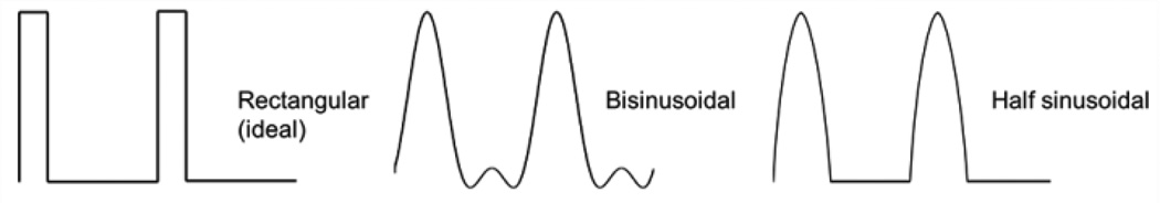
Most used asymmetric waveform profiles in FAIMS.
For each different waveform its portion of high electric field will be different, so the ions movement inside the filtering electrodes gap will also be different for each waveform and, therefore, the detected compensation voltage. Prieto et al.164 studied how the shape of the waveform applied affected the compensation voltage for the bisinusoidal and the rectangular waveforms. Figure 19 shows CV as a function of DV for square and sinusoidal waveforms, with the bisinusoidal wave at 750 kHz and for a duty cycle of 33.3 %; and the square wave at three different frequencies (250, 333, and 500 kHz), all with a duty cycle of 25 %. Compensation voltages from each waveform considered differ by 0.7 V for a dispersion field of 300 V, and by 1.0 V for a dispersion field of 350 V.
Figure 19.

Graph displaying behaviour of CV as a function of DV for a rectangular and a bisinusoidal waveform. Adapted with permission from 164. Copyright (2011) American Chemical Society.
3.5 Humidity, Temperature and Pressure Effects
The importance of humidity and temperature in overall performance of ion mobility methods can hardly be overstated and is certainly the most significant of parameters that can be controlled on most analysers. Operating mobility analysers without knowledge of these two parameters is equivalent to making measurements in MS without knowledge or control of the vacuum. Remarkably, mobility spectrometers function well across a wide range of humidity levels and temperatures, yet without control of theses parameters, response and reproducibility will be difficult to understand, and comparison between laboratories may be difficult to achieve with a high level of confidence. Although fundamental measurements of association energies of gas phase protons with water molecules were made in the early 1970s169, 170, the importance on response has been experimentally explored only in the past two decades for atmospheric pressure ionization (API) MS171, 172 and only recently for IMS36, 157, 173–175.
Drift time varies linearly with pressure while it does not change linearly with temperature176. This different behaviour was attributed to the different impact of temperature and pressure on the clustering reactions. In fact, temperature and pressure both affect the neutral density of the drift gas, which leads to a change in the collision frequency. However, temperature changes the identity of the ions by affecting the clustering equilibrium. Thus, a non-linear behaviour is observed for temperature but not for pressure.
1. Humidity effects
Vautz et al. studied how humidity affected the spectrum of a single compound36 with a UV-IMS. Figure 20a presents the IMS spectra of trimethylamine (TMA) in purified air for a varying relative humidity (RH). TMA is involved in atmospheric nucleation, i.e. the natural process whereby new particles are generated175.
Figure 20.

(a) Spectra of TMA at a constant concentration (220 ppb) measured with high concentrations of water vapour. (b) The relationships between water concentration and drift times of the reactant ions and the monomer ions. Reprinted from Ref. 175. Copyright (2011) with permission from Elsevier.
Mäkinen et. al175 studied relative humidity variations between 10% and 70% (∼2300ppm and 16,500 ppm, respectively). As seen, the peak representing dimer structures is only present in the “dry” spectrum measured without any additional humidity. The explicit shift of monomer and RIP peaks rightwards (towards longer drift times) is directly related to the increase of water amount, being the relationship between humidity and peak positions presented in Figure 20b.
When adding humidity to complex samples like breath, additional peaks can result of cluster reactions in the presence of water molecules. For dry air, only two major peaks are obtained: monomer MH+ and dimer M2H+ of the analyte M. When adding water molecules, hydration reactions (formation of ion clusters) happen, and different clusters can be obtained depending on the number of water molecules attached3 (n): M (H2O)nH+ for monomers and M2(H2O)nH+ for dimmers. As more humidity is added more ion-water clusters are obtained, leading to a decrease of the intensity of monomers and dimers, making the identification of the substance much more difficult. The effects of variations in humidity with FAIMS are the same if we consider ion formation. However, as FAIMS operates at high-fields consequences are distinctive to this method. Krylova et.al157, 177 studied the humidity influence in detail using a set of organophosphorus compounds (OPCs) in a planar-FAIMS or DMS. They studied how humidity affects the mobility coefficient dependence with the field for E/N values from 0 to 140 Td. E/N is expressed in V·cm2, where N is the number density (the number of molecules per unit volume), but for convenience, it was resolved to adopt the unit Townsend169, 170: 1 Td = 10−21 V·m2. The mobility of an ion under the effects of high electrical fields where FAIMS are operated can be expressed empirically by [300]:
| (22) |
where K0 = K(E)|E = 0 is the mobility of the ion for a low electrical field where are operated the conventional drift time IMS, and the function α(E/N) takes account of the dependence of the ion mobility with the electrical field for a constant gas density. At moisture levels of 0.1 to 10 ppm, the alpha function for protonated monomers was unchanged. At 50 ppm, there was an onset of change in the alpha function that was doubled when moisture level was raised from 100 to 1,000 ppm at all E/N values. Changes of the alpha function with humidity continued with another doubled increase from 1,000 to 10,000 ppm of humidity. In Figure 21 are shown alpha plots for organophosphorus compounds at two levels of moisture, showing clearly different alpha values depending on the humidity content.
Figure 21.

Alpha plots for organo-phosphorus compounds at two levels of moisture. The top frame is high moisture and the bottom frame is low moisture. Adapted with permission from Ref. 157. Copyright (2003) American Chemical Society.
2. Temperature and pressure effects
Temperature and pressure effects in ion separation can be described by the mobility dependence on the gas number density, N: K(E/N) defined in Equation (22) and from Equations:
| (23) |
| (24) |
| (25) |
The number density N [m−3] can be found using Equation (23), where n/V [mol·m−3] is determined from the ideal gas law in Equation (24) and NA [6.022×10²³ mol−1] is Avogadro’s number. Also, p [Pa] is the pressure of the gas, V [m3] is the volume of the gas, n [mol] is the amount of substance of gas (also known as number of moles), T [K] is the temperature of the gas and R [8.314 J·K−1·mol−1] is the ideal, or universal, gas constant, equal to the product of the Boltzmann constant [1.38065 × 10⁻²³ J·K−1] and the Avogadro number NA.
From previous equations, it is determined that as temperature T increases, n/V decreases causing the number density to decrease and therefore the effective E/N to increase. On the other hand, it is determined that as pressure p increases, n/V also increases causing the number density to increase and therefore the effective E/N to decrease. Thus, to maintain balanced conditions for an ion of interest, temperature and pressure conditions must be constant.
The effect of temperature in ion mobility has been widely studied, but mainly restricted to studies of the relationship for drift time (td) vs. temperature of positive ions without consideration of quantitative effects178. According to ion mobility theory, a linear proportionality of 1/td to the absolute temperature and the reciprocal pressure can be expected176. In contrast to a linear relationship between drift times and pressure, the interrelation between drift times and temperature were found to be non-linear due to differences in hydration and clustering27. Higher temperatures are associated with a lower degree of clustering because neutral vapours will detach themselves from the primary ion179. In addition to these processes, also the formation of positive fragment ions can be affected by temperature. Depending on the functional groups, the comparison of ion mobility measurements at low and elevated temperatures permits the identification of different chemical classes180. Furthermore, elevated temperatures cause an increasing resolving power due to the reduced effect hydration and clustering. In contrast, negative ion mobility spectra are better resolved at elevated temperatures181. A differentiation between the halide production peaks is possible at elevated temperatures (Figure 22)181. Also, increasing peak-to-peak resolutions were observed for negative productions of CHCl3, CHBr3 and CH3I at elevated temperatures98.
Figure 22.

Ion mobility spectra of 1-halo-hexanes obtained at 70 and 150°C using a regular IMS. Reprinted from Ref. 181. Copyright (2012) with permission from Elsevier.
In planar-FAIMS or DMS it has been shown that pressure influence in p-FAIMS peak positions may be eliminated by a rescaling of the coordinates, expressing both compensation and separation fields in Townsend units (electric field divided by density)144. At fixed temperature, Townsend-rescaled p-FAIMS spectra are independent of the drift gas pressure (see Figure 23a). In contrast, p-FAIMS spectra recorded at fixed pressure but varying temperature do not simplify in a similar way182. Even in terms of Townsend p-FAIMS spectra are distinguished by different bulk temperatures (see Figure 23b). In measurements with asymmetric waveforms with field extremes, at ambient pressure, of −1,000 to 30,000 V/cm or greater, ions are near thermalized in the low portion of the waveform (−1,000 V/cm); however, ions are heated by the electric field during the high portion of the waveform when the energy from the field is large compared to thermal energy. This causes an increase in ion temperature in a cooler surrounding gas atmosphere.
Figure 23.

Positive p-FAIMS spectra of methyl salicylate ions at the same 100 Td filtering field, but with different drift gas pressures (a) and temperatures (b). Pressure does not affect the p-FAIMS spectrum scaled in Td units. Variation of peak position with temperature remains even after Townsend scaling. Reprinted from Ref. 182, Copyright (2009) with permission from Elsevier.
Summary and Future Trends
Ion mobility spectrometry offers a range of applications and possibilities for use in field, medical and process analytical applications. The specificity of IMS is dependent upon ion source and sample concentration and the linear range can be high due to a combination of drift time and ionization properties (dependent upon the ion source). Though mobility was once restricted to small ions or molecules, the method now can be seen as a general analytical method dependent only upon the methods used to form product ions from a sample. Advances during the past decade have included improvements in the understandings of gas-phase ion chemistry that underlies the appearance of mobility spectra, in technique to create gas-phase ions, in technology and manufacture of drift tubes, and in the growth of new field-dependent mobility methods. An extended summary of reported effects of experimental parameters is reported for IMS and FAIMS devices.
When unfavourable conditions exist, hyphenated techniques are preferable, mainly Gas Chromatography other Mass Spectrometry. In terms of consumption, IMS is more suitable than mass spectrometry and gas chromatography, since it does not consume gas, does not require a vacuum, and draws relatively little power (batteries are often sufficient). The availability of analysers for general use from instrument vendors may initiate a new stage of development with IMS and FAIMS.
Acknowledgements
The long term relation, fruitful discussions and scientific cooperation with G.A. Eiceman (NMSU, Las Cruces, NM, USA) should be mentioned thankfully. Part of this work and the PhD Thesis grant of Dr. R. Cumeras have been financially supported by the Spanish Ministry of Science and Innovation MICINN-TEC2007-67962-C04 project, and MICIIN-TEC2010-21357-C05 project. Part of the work of this paper has been supported by the Deutsche Forschungsgemeinschaft (DFG) within the Collaborative Research Center (Sonderforschungsbereich) SFB 876 Providing Information by Resource-Constrained Analysis, project TB1 Resource-Constrained Analysis of Spectrometry Data (JIBB). Other partial support was provided by The Hartwell Foundation, the National Science Foundation grant #1255915, and the National Center for Advancing Translational Sciences (NCATS) of the NIH grant #UL1 TR000002 (CED).
references
- 1.Borsdorf H, Eiceman GA. Appl. Spectrosc. Rev. 2006;41:323–375. [Google Scholar]
- 2.Hill HH, Siems WF, St Louis RW, McMinn DG. Anal. Chem. 1990;62:1201A–1209A. doi: 10.1021/ac00222a001. [DOI] [PubMed] [Google Scholar]
- 3.Cumeras R, Figueras E, Davis CE, Baumbach JI, Gràcia I. Analyst. 2014 [Google Scholar]
- 4.Buryakov IA, Krylov EV, Nazarov EG, Rasulev UK. Int. J. Mass Spectr. Ion Proc. 1993;128:143–148. [Google Scholar]
- 5.Eiceman GA, Karpas Z. Ion Mobility Spectrometry. 2nd edn. Boca Raton: CRC Press; 2005. [Google Scholar]
- 6.Vautz W, Baumbach J, Westhoff M, Züchner K, Carstens E, Perl T. Int. J. Ion Mobil. Spec. 2010;13:41–46. [Google Scholar]
- 7.Ruzsanyi V, Baumbach JI, Sielemann S, Litterst P, Westhoff M, Freitag L. J. Chromatogr. A. 2005;1084:145–151. doi: 10.1016/j.chroma.2005.01.055. [DOI] [PubMed] [Google Scholar]
- 8.Vautz W, Bödeker B, Baumbach JI, Bader S, Westhoff M, Perl T. Int. J. Ion Mobil. Spec. 2009;12:47–57. [Google Scholar]
- 9.Baumbach JI, Vautz W, Ruzsanyi V, Freitag L. In: Modern Biopharmaceuticals. Knäblein J, editor. Vol. 3. Wiley-VCH Weinheim; 2005. pp. 1343–1358. [Google Scholar]
- 10.Jünger M, Bödeker B, Baumbach JI. Anal. Bioanal. Chem. 2010;396:471–482. doi: 10.1007/s00216-009-3168-z. [DOI] [PubMed] [Google Scholar]
- 11.Basanta M, Jarvis RM, Xu Y, Blackburn G, Tal-Singer R, Woodcock A, Singh D, Goodacre R, Thomas CLP, Fowler SJ. Analyst. 2010;135:315–320. doi: 10.1039/b916374c. [DOI] [PubMed] [Google Scholar]
- 12.Baumbach JI, Westhoff M. Spectroscopy Europe. 2006;18:22–27. [Google Scholar]
- 13.Ruzsanyi V, Baumbach JI, Eiceman GA. Int. J. Ion Mobil. Spec. 2003;6:53–58. [Google Scholar]
- 14.Prasad S, Pierce KM, Schmidt H, Rao JV, Gueth R, Bader S, Synovec RE, Smith GB, Eiceman GA. Analyst. 2007;132:1031–1039. doi: 10.1039/b705929a. [DOI] [PubMed] [Google Scholar]
- 15.Prasad S, Schmidt H, Lampen P, Wang M, Guth R, Rao JV, Smith GB, Eiceman GA. Analyst. 2006;131:1216–1225. doi: 10.1039/b608127d. [DOI] [PubMed] [Google Scholar]
- 16.Chaim W, Karpas Z, Lorber A. Eur. J. Obstet. Gynecol. Reprod. Biol. 2003;111:83–87. doi: 10.1016/s0301-2115(03)00210-0. [DOI] [PubMed] [Google Scholar]
- 17.Karpas Z, Tilman B, Gdalevsky R, Lorber A. Anal. Chim. Acta. 2002;463:155–163. [Google Scholar]
- 18.Snyder AP, Dworzanski JP, Tripathi A, Maswadeh WM, Wick CH. Anal. Chem. 2004;76:6492–6499. doi: 10.1021/ac040099i. [DOI] [PubMed] [Google Scholar]
- 19.Harrington Pd. B, Buxton TL, Chen G. Int. J. Ion Mobil. Spec. 2001;4:148–151. [Google Scholar]
- 20.Shnayderman M, Mansfield B, Yip P, Clark HA, Krebs MD, Cohen SJ, Zeskind JE, Ryan ET, Dorkin HL, Callahan MV, Stair TO, Gelfand JA, Gill CJ, Hitt B, Davis CE. Anal. Chem. 2005;77:5930–5937. doi: 10.1021/ac050348i. [DOI] [PubMed] [Google Scholar]
- 21.Venne K, Bonneil E, Eng K, Thibault P. Anal. Chem. 2005;77:2176–2186. doi: 10.1021/ac048410j. [DOI] [PubMed] [Google Scholar]
- 22.Handy R, Barnett DA, Purves RW, Horlick G, Guevremont R. J. Anal. Atom. Spectrom. 2000;15:907–911. [Google Scholar]
- 23.Levin DS, Vouros P, Miller RA, Nazarov EG, Morris JC. Anal. Chem. 2006;78:96–106. doi: 10.1021/ac051217k. [DOI] [PubMed] [Google Scholar]
- 24.Steiner WE, Klopsch SJ, English WA, Clowers BH, Hill HH. Anal. Chem. 2005;77:4792–4799. doi: 10.1021/ac050278f. [DOI] [PubMed] [Google Scholar]
- 25.Metz TO, Page JS, Baker ES, Tang K, Ding J, Shen Y, Smith RD. Trac-trend. Anal. Chem. 2008;27:205–214. doi: 10.1016/j.trac.2007.11.003. [DOI] [PMC free article] [PubMed] [Google Scholar]
- 26.Waters Corp. 2013 vol. [Google Scholar]
- 27.Kanu AB, Hill HH. J. Chromatogr. A. 2008;1177:12–27. doi: 10.1016/j.chroma.2007.10.110. [DOI] [PubMed] [Google Scholar]
- 28.Owlstone Nanotech INC. 2013 vol. [Google Scholar]
- 29.Lambertus GR, Fix CS, Reidy SM, Miller RA, Wheeler D, Nazarov EG, Sacks R. Anal. Chem. 2005;77:7563–7571. doi: 10.1021/ac051216s. [DOI] [PubMed] [Google Scholar]
- 30.Eiceman GA, Nazarov EG, Miller RA, Krylov EV, Zapata AM. Analyst. 2002;127:466–471. doi: 10.1039/b111547m. [DOI] [PubMed] [Google Scholar]
- 31.Basanta M, Singh D, Fowler S, Wilson I, Dennis R, Thomas CLP. J. Chromatogr. A. 2007;1173:129–138. doi: 10.1016/j.chroma.2007.09.082. [DOI] [PubMed] [Google Scholar]
- 32.Lu Y, Harrington PB. Anal. Chem. 2007;79:6752–6759. doi: 10.1021/ac0707028. [DOI] [PubMed] [Google Scholar]
- 33.Vautz W, Baumbach JI. Int. J. Ion Mobil. Spec. 2008;11:35–42. [Google Scholar]
- 34.Westhoff M, Litterst P, Freitag L, Urfer W, Bader S, Baumbach JI. Thorax. 2009;64:744–748. doi: 10.1136/thx.2008.099465. [DOI] [PubMed] [Google Scholar]
- 35.Limero T, Reese E, Wallace W, Cheng P, Trowbridge J. Int. J. Ion Mobil. Spec. 2012;15:189–198. [Google Scholar]
- 36.Vautz W, Ruszany V, Sielemann S, Baumbach JI. Int. J. Ion Mobil. Spec. 2004;7:3–8. [Google Scholar]
- 37.Schwanhausser B, Busse D, Li N, Dittmar G, Schuchhardt J, Wolf J, Chen W, Selbach M. Nature. 2011;473:337–342. doi: 10.1038/nature10098. [DOI] [PubMed] [Google Scholar]
- 38.Clowers BH, Ibrahim YM, Prior DC, Danielson WF, Belov ME, Smith RD. Anal. Chem. 2008;80:612–623. doi: 10.1021/ac701648p. [DOI] [PMC free article] [PubMed] [Google Scholar]
- 39.Belov ME, Buschbach MA, Prior DC, Tang K, Smith RD. Anal. Chem. 2007;79:2451–2462. doi: 10.1021/ac0617316. [DOI] [PMC free article] [PubMed] [Google Scholar]
- 40.Liu Z, Patterson DG, Lee ML. Anal. Chem. 1995;67:3840–3845. [Google Scholar]
- 41.Ruotolo BT, Gillig KJ, Stone EG, Russell DH. J. Chromatogr. B. 2002;782:385–392. doi: 10.1016/s1570-0232(02)00566-4. [DOI] [PubMed] [Google Scholar]
- 42.Glish GL, Vachet RW. Nat. Rev. Drug Discov. 2003;2:140–150. doi: 10.1038/nrd1011. [DOI] [PubMed] [Google Scholar]
- 43.Kanu AB, Dwivedi P, Tam M, Matz L, Hill HH. J. Mass Spectrom. 2008;43:1–22. doi: 10.1002/jms.1383. [DOI] [PubMed] [Google Scholar]
- 44.McDaniel EW, Martin DW, Barnes WS. Rev. Sci. Instrum. 1962;33:2–7. [Google Scholar]
- 45.Pringle SD, Giles K, Wildgoose JL, Williams JP, Slade SE, Thalassinos K, Bateman RH, Bowers MT, Scrivens JH. Int. J. Mass Spectrom. 2007;261:1–12. [Google Scholar]
- 46.Mukhopadhyay R. Anal. Chem. 2008;80:7918–7920. doi: 10.1021/ac8018608. [DOI] [PubMed] [Google Scholar]
- 47.Bohrer BC, Merenbloom SI, Koeniger SL, Hilderbrand AE, Clemmer DE. Annu. Rev. Anal. Chem. 2008;1:293–327. doi: 10.1146/annurev.anchem.1.031207.113001. [DOI] [PMC free article] [PubMed] [Google Scholar]
- 48.May JC, Goodwin CR, Lareau NM, Leaptrot KL, Morris CB, Kurulugama RT, Mordehai A, Klein C, Barry W, Darland E, Overney G, Imatani K, Stafford GC, Fjeldsted JC, McLean JA. Anal. Chem. 2014 doi: 10.1021/ac4038448. [DOI] [PMC free article] [PubMed] [Google Scholar]
- 49.Both P, Green AP, Gray CJ, Šardzík R, Voglmeir J, Fontana C, Austeri M, Rejzek M, Richardson D, Field RA, Widmalm G, Flitsch SL, Eyers CE. Nat. Chem. 2014;6:65–74. doi: 10.1038/nchem.1817. [DOI] [PubMed] [Google Scholar]
- 50.Uetrecht C, Barbu IM, Shoemaker GK, van Duijn E, HeckAlbert JR. Nat. Chem. 2011;3:126–132. doi: 10.1038/nchem.947. [DOI] [PubMed] [Google Scholar]
- 51.Lanucara F, Holman SW, Gray CJ, Eyers CE. Nat. Chem. 2014;6:281–294. doi: 10.1038/nchem.1889. [DOI] [PubMed] [Google Scholar]
- 52.Lopez A, Tarrago T, Vilaseca M, Giralt E. New J. Chem. 2013;37:1283–1289. [Google Scholar]
- 53.A. S. Inc. 2013 vol. [Google Scholar]
- 54.T. S. Inc. 2013 vol. [Google Scholar]
- 55.Tang KQ, Li FM, Shvartsburg AA, Strittmatter EF, Smith RD. Anal. Chem. 2005;77:6381–6388. doi: 10.1021/ac050871x. [DOI] [PMC free article] [PubMed] [Google Scholar]
- 56.Shvartsburg AA, Li F, Tang K, Smith RD. Anal. Chem. 2006;78:3706–3714. doi: 10.1021/ac052020v. [DOI] [PMC free article] [PubMed] [Google Scholar]
- 57.2011 8299443 B1. [Google Scholar]
- 58.National Institute of Standards and Technology (NIST) 2014 vol. [Google Scholar]
- 59.WILEY. 2014 vol. [Google Scholar]
- 60.Bushnell JE, Kemper PR, Bazan GC, Bowers MT. J. Phys. Chem. A. 2004;108:7730–7735. [Google Scholar]
- 61.Baker ES, Hong JW, Gidden J, Bartholomew GP, Bazan GC, Bowers MT. J. Am. Chem. Soc. 2004;126:6255–6257. doi: 10.1021/ja039486k. [DOI] [PubMed] [Google Scholar]
- 62.Perl T, Bödecker B, Jünger M, Nolte J, Vautz W. Anal. Bioanal. Chem. 2010;397:2385–2394. doi: 10.1007/s00216-010-3798-1. [DOI] [PMC free article] [PubMed] [Google Scholar]
- 63.SGE Analytical Science. 2013 vol. [Google Scholar]
- 64.Baumbach JI. J. Breath Res. 2009;3:1–16. doi: 10.1088/1752-7155/3/3/034001. [DOI] [PubMed] [Google Scholar]
- 65.Anderson AG, Markoski KA, Shi Q, Coy SL, Krylov EV, Nazarov EG. 2008 69540H-69540H. [Google Scholar]
- 66.Eiceman GA, Karpas Z, Hill HH., Jr. Ion Mobility Spectrometry. 3rd edn. CRC Press: Boca Raton; 2014. [Google Scholar]
- 67.Menlyadiev MR, Eiceman GA. Anal. Chem. 2014;86:2395–2402. doi: 10.1021/ac4031169. [DOI] [PubMed] [Google Scholar]
- 68.Merenbloom SI, Koeniger SL, Valentine SJ, Plasencia MD, Clemmer DE. Anal. Chem. 2006;78:2802–2809. doi: 10.1021/ac052208e. [DOI] [PubMed] [Google Scholar]
- 69.Kurulugama RT, Valentine SJ, Sowell RA, Clemmer DE. J. Proteomics. 2008;71:318–331. doi: 10.1016/j.jprot.2008.06.010. [DOI] [PMC free article] [PubMed] [Google Scholar]
- 70.Li Z, Valentine S, Clemmer D. J. Am. Soc. Mass Spectr. 2011;22:817–827. doi: 10.1007/s13361-011-0105-0. [DOI] [PMC free article] [PubMed] [Google Scholar]
- 71.Atlasevich N, Holliday AE, Valentine SJ, Clemmer DE. J. Phys. Chem. B. 2012;116:7644–7651. doi: 10.1021/jp303778w. [DOI] [PMC free article] [PubMed] [Google Scholar]
- 72.Maddula S, Rupp K, Baumbach J. Int. J. Ion Mobil. Spec. 2012;15:79–81. [Google Scholar]
- 73.Bunkowski A. Int. J. Ion Mobil. Spec. 2010;13:169–175. [Google Scholar]
- 74.Maurer F, Hauschild AC, Eisinger K, Baumbach J, Mayor A, Baumbach JI. Int. J. Ion Mobil. Spec. 2014:1–7. [Google Scholar]
- 75.Max Planck Institute Informatik and KIST Europe. 2014 vol. [Google Scholar]
- 76.Crawford C, Graf S, Gonin M, Fuhrer K, Zhang X, Hill H., Jr. Int. J. Ion Mobil. Spec. 2011;14:23–30. [Google Scholar]
- 77.Shliaha PV, Bond NJ, Gatto L, Lilley KS. J. Proteome Res. 2013;12:2323–2339. doi: 10.1021/pr300775k. [DOI] [PubMed] [Google Scholar]
- 78.Shvartsburg AA, Smith RD. Anal. Chem. 2008;80:9689–9699. doi: 10.1021/ac8016295. [DOI] [PMC free article] [PubMed] [Google Scholar]
- 79.Giles K, Pringle SD, Worthington KR, Little D, Wildgoose JL, Bateman RH. Rapid Commun. Mass Spectrom. 2004;18:2401–2414. doi: 10.1002/rcm.1641. [DOI] [PubMed] [Google Scholar]
- 80.Baker ES, Livesay EA, Orton DJ, Moore RJ, Danielson WF, Prior DC, Ibrahim YM, LaMarche BL, Mayampurath AM, Schepmoes AA, Hopkins DF, Tang K, Smith RD, Belov ME. J. Proteome Res. 2009;9:997–1006. doi: 10.1021/pr900888b. [DOI] [PMC free article] [PubMed] [Google Scholar]
- 81.Valentine SJ, Plasencia MD, Liu X, Krishnan M, Naylor S, Udseth HR, Smith RD, Clemmer DE. J. Proteome Res. 2006;5:2977–2984. doi: 10.1021/pr060232i. [DOI] [PubMed] [Google Scholar]
- 82.Geromanos SJ, Hughes C, Ciavarini S, Vissers JPC, Langridge JI. Anal. Bioanal. Chem. 2012;404:1127–1139. doi: 10.1007/s00216-012-6197-y. [DOI] [PubMed] [Google Scholar]
- 83.Valentine SJ, Counterman AE, Hoaglund CS, Reilly JP, Clemmer DE. J. Am. Soc. Mass Spectr. 1998;9:1213–1216. doi: 10.1016/S1044-0305(98)00101-9. [DOI] [PubMed] [Google Scholar]
- 84.Cuyckens F, Wassvik C, Mortishire-Smith RJ, Tresadern G, Campuzano I, Claereboudt J. Rapid Commun. Mass Spectrom. 2011;25:3497–3503. doi: 10.1002/rcm.5258. [DOI] [PubMed] [Google Scholar]
- 85.Dear GJ, Munoz-Muriedas J, Beaumont C, Roberts A, Kirk J, Williams JP, Campuzano I. Rapid Commun. Mass Spectrom. 2010;24:3157–3162. doi: 10.1002/rcm.4742. [DOI] [PubMed] [Google Scholar]
- 86.Hoaglund CS, Valentine SJ, Clemmer DE. Anal. Chem. 1997;69:4156–4161. [Google Scholar]
- 87.Davis EJ, Grows KF, Siems WF, Hill HH. Anal. Chem. 2012;84:4858–4865. doi: 10.1021/ac300452j. [DOI] [PubMed] [Google Scholar]
- 88.Smiths Detection. 2014 vol. [Google Scholar]
- 89.Morpho Detection Inc. 2013 vol. [Google Scholar]
- 90.Environics Oy. 2013 vol. [Google Scholar]
- 91.Chemring Group Plc. 2013 vol. [Google Scholar]
- 92.IUPAC. 2013 vol. [Google Scholar]
- 93.Davis EJ, Dwivedi P, Tam M, Siems WF, Hill HH. Anal. Chem. 2009;81:3270–3275. doi: 10.1021/ac802431q. [DOI] [PMC free article] [PubMed] [Google Scholar]
- 94.Cohen MJ, Karasek FW. J. Chromatogr. Sci. 1970;8:330–337. [Google Scholar]
- 95.Asbury GR, Hill HH. J. Microcolumn Sep. 2000;12:172–178. [Google Scholar]
- 96.Rokushika S, Hatano H, Baim MA, Hill HH. Anal. Chem. 1985;57:1902–1907. [Google Scholar]
- 97.Tabrizchi M, Rouholahnejad F. Talanta. 2006;69:87–90. doi: 10.1016/j.talanta.2005.09.016. [DOI] [PubMed] [Google Scholar]
- 98.Tabrizchi M. Talanta. 2004;62:65–70. doi: 10.1016/S0039-9140(03)00401-6. [DOI] [PubMed] [Google Scholar]
- 99.Siems WF, Wu C, Tarver EE, Hill HH, Larsen PR, McMinn DG. Anal. Chem. 1994;66:4195–4201. [Google Scholar]
- 100.D. C. Harris. Freeman WH. Quantitative Chemcial Analysis. 2011 [Google Scholar]
- 101.Rorrer LC, III, Yost RA. Int. J. Mass Spectrom. 2011;300:173–181. [Google Scholar]
- 102.Revercomb HE, Mason EA. Anal. Chem. 1975;47:970–983. [Google Scholar]
- 103.Louis RHSt, Hill HH., Jr. Crit. Rev. Anal. Chem. 1990;21:321–355. [Google Scholar]
- 104.Krylov EV. Int. J. Mass Spectrom. 2003;225:39–51. [Google Scholar]
- 105.Miller RA, Eiceman GA, Nazarov EG, King AT. Sens. Actuator B-Chem. 2000;67:300–306. [Google Scholar]
- 106.Babis JS, Sperline RP, Knight AK, Jones DA, Gresham CA, Denton MB. Anal. Bioanal. Chem. 2009;395:411–419. doi: 10.1007/s00216-009-2818-5. [DOI] [PubMed] [Google Scholar]
- 107.Baumbach JI, Sielemann S, Pilzecker P. Int. J. Ion Mobil. Spec. 2000;3:28–37. [Google Scholar]
- 108.Kanu AB, Gribb MM, Hill HH. Anal. Chem. 2008;80:6610–6619. doi: 10.1021/ac8008143. [DOI] [PMC free article] [PubMed] [Google Scholar]
- 109.Kang WJ, Teepe M, Neyer A, Baumbach JI, Schmidt H, Sielemann S. Int. J. Ion Mobil. Spec. 2001;4:108–111. [Google Scholar]
- 110.Teepe M, Baumbach JI, Neyer A, Schmidt H, Pilzecker P. Int. J. Ion Mobil. Spec. 2001;4:60–64. [Google Scholar]
- 111.Pfeifer KB, Sanchez RC. Int. J. Ion Mobil. Spec. 2002;5:63–66. [Google Scholar]
- 112.Xu J, Whitten WB, Ramsey JM. Int. J. Ion Mobil. Spec. 2002;5:207–214. [Google Scholar]
- 113.Zimmermann S, Barth S, Baether WKM, Ringer J. Anal. Chem. 2008;80:6671–6676. doi: 10.1021/ac800559h. [DOI] [PubMed] [Google Scholar]
- 114.Lamabadusuriya MR, Siems WF, Hill HH, Mariano A, Guharay SK. Anal. Chem. 2012;84:9295–9302. doi: 10.1021/ac302022d. [DOI] [PubMed] [Google Scholar]
- 115.Mariano AV, Su W, Guharay SK. Anal. Chem. 2009;81:3385–3391. doi: 10.1021/ac802652f. [DOI] [PubMed] [Google Scholar]
- 116.Tarver EE. Sensors. 2004;4:1–13. [Google Scholar]
- 117.Guideline IHT. 2013 vol. [Google Scholar]
- 118.2013 E. P. 5.0. vol. [Google Scholar]
- 119.Davis DM, Harden CS, Shoff DB, Bell SE, Eiceman GA, Ewing RG. Anal. Chim. Acta. 1994;289:263–272. [Google Scholar]
- 120.Vogtland D, Baumbach JI. Int. J. Ion Mobil. Spec. 2009;12:109–114. [Google Scholar]
- 121.Cumeras R, Schneider T, Favrod P, Figueras E, Gràcia I, Maddula S, Baumbach JI. Int. J. Ion Mobil. Spec. 2012;15:41–46. [Google Scholar]
- 122.NIST/SEMATECH [Google Scholar]
- 123.Smolinska A, Hauschild AC, Fijten RRR, Dallinga JW, Baumbach J, Schooten FJv. J. Breath Res. 2014;8:027105. doi: 10.1088/1752-7155/8/2/027105. [DOI] [PubMed] [Google Scholar]
- 124.Banach U, Tiebe C, Hübert T. Food Control. 2012;26:23–27. [Google Scholar]
- 125.Shvartsburg AA, Tang K, Smith RD. Anal. Chem. 2004;76:7366–7374. doi: 10.1021/ac049299k. [DOI] [PubMed] [Google Scholar]
- 126.Kim SH, Karasek FW, Rokushika S. Anal. Chem. 1978;50:152–155. [Google Scholar]
- 127.Blyth DA. Proc. Int. Symp. on Protection against Chem. Warfare. 1983 [Google Scholar]
- 128.Spangler GE, Carrico JP, Campbell DN. J. Test. Eval. 1985;13:234–240. [Google Scholar]
- 129.Eiceman GA, Wang YF, Garcia-Gonzalez L, Harden CS, Shoff DB. Anal. Chim. Acta. 1995;306:21–33. [Google Scholar]
- 130.Meng Q, Karpas Z, Eiceman GA. Int. J. Environ. Anal. Chem. 1995;61:81–94. [Google Scholar]
- 131.Fernández-Maestre R, Wu C, Hill HH. Rapid Commun. Mass Spectrom. 2012;26:2211–2223. doi: 10.1002/rcm.6335. [DOI] [PMC free article] [PubMed] [Google Scholar]
- 132.Fernández-Maestre R, Wu C, Hill HH., Jr Int. J. Mass Spectrom. 2010;298:2–9. doi: 10.1016/j.ijms.2010.08.009. [DOI] [PMC free article] [PubMed] [Google Scholar]
- 133.Shvartsburg AA, Smith RD. Anal. Chem. 2011;83:9159–9166. doi: 10.1021/ac202386w. [DOI] [PMC free article] [PubMed] [Google Scholar]
- 134.Niemann HB, Atreya SK, Carignan GR, Donahue TM, Haberman JA, Harpold DN, Hartle RE, Hunten DM, Kasprzak WT, Mahaffy PR, Owen TC, Spencer NW, Way SH. Science. 1996;272:846–849. doi: 10.1126/science.272.5263.846. [DOI] [PubMed] [Google Scholar]
- 135.Hanel R, Conrath B, Flasar FM, Kunde V, Maguire W, Pearl J, Pirraglia J, Samuelson R, Herath L, Allison M, Cruikshank D, Gautier D, Gierasch P, Horn L, Koppany R, Ponnamperuma C. Science. 1981;212:192–200. doi: 10.1126/science.212.4491.192. [DOI] [PubMed] [Google Scholar]
- 136.Puton J, Nousiainen M, Sillanpää M. Talanta. 2008;76:978–987. doi: 10.1016/j.talanta.2008.05.031. [DOI] [PubMed] [Google Scholar]
- 137.Ross SK, McDonald G, Marchant S. Analyst. 2008;133:602–607. doi: 10.1039/b801457b. [DOI] [PubMed] [Google Scholar]
- 138.Barnett DA, Ells B, Guevremont R, Purves RW, Viehland LA. J. Am. Soc. Mass Spectr. 2000;11:1125–1133. doi: 10.1016/S1044-0305(00)00187-2. [DOI] [PubMed] [Google Scholar]
- 139.Krylov EV, Nazarov EG, Miller RA. Int. J. Mass Spectrom. 2007;266:76–85. [Google Scholar]
- 140.Shvartsburg AA. Differential Ion Mobility Spectrometry: Nonlinear Ion Transport and Fundamentals of FAIMS. First edn. Boca Raton, FL: CRC Press; 2009. [Google Scholar]
- 141.Spangler GE. Anal. Chem. 1992;64:1312–1312. [Google Scholar]
- 142.NIST. 2013 vol. [Google Scholar]
- 143.Guevremont R, Purves R. J. Am. Soc. Mass Spectr. 2005;16:349–362. doi: 10.1016/j.jasms.2004.11.013. [DOI] [PubMed] [Google Scholar]
- 144.Nazarov EG, Coy SL, Krylov EV, Miller RA, Eiceman GA. Anal. Chem. 2006;78:7697–7706. doi: 10.1021/ac061092z. [DOI] [PubMed] [Google Scholar]
- 145.Mason EA, McDaniel EW. Transport properties of ions in gases. New York: John Wiley & Sons Inc; 1988. [Google Scholar]
- 146.Eiceman GA, Bergloff JF, Rodriguez JE, Munro W, Karpas Z. J. Am. Soc. Mass Spectr. 1999;10:1157–1165. doi: 10.1016/S1044-0305(99)00082-3. [DOI] [PubMed] [Google Scholar]
- 147.Paschen F. Ann. Phys.-Berlin. 1889;273:69–96. [Google Scholar]
- 148.Bazelyan EM, Raizer YP. Spark Discharge. 1998 [Google Scholar]
- 149.Wallash AJ, Levit L. Proc. SPIE 4980, Reliability, Testing, and Characterization of MEMS/MOEMS II. 2003:87. vol. [Google Scholar]
- 150.Livermore C. Massachusetts Institute of Technology. 2007 Spring; MIT Open Course Ware ( http://ocw.mit.edu/) Downloaded on [24 April 2013] [Google Scholar]
- 151.Hourdakis E, Simonds BJ, Zimmerman NM. Rev. Sci. Instrum. 2006;77:034702–034704. [Google Scholar]
- 152.Hourdakis E, Bryant GW, Zimmerman NM. J. Appl. Phys. 2006;100:123306–123306. [Google Scholar]
- 153.Carazzetti P, Shea HR. J. Micro/Nanolith. MEMS MOEMS. 2009;8 031305-031305-031309. [Google Scholar]
- 154.Tirumala R, Go DB. Appl. Phys. Lett. 2010;97 [Google Scholar]
- 155.Go DB, Pohlman DA. J. Appl. Phys. 2010;107 [Google Scholar]
- 156.Marcis Y. Ion Solvation. Wiley-Interscience; 1985. [Google Scholar]
- 157.Krylova N, Krylov E, Eiceman GA, Stone JA. J. Phys. Chem. A. 2003;107:3648–3654. doi: 10.1021/jp0221136. [DOI] [PubMed] [Google Scholar]
- 158.Eiceman GA, Krylov EV, Nazarov EG, Miller RA. Anal. Chem. 2004;76:4937–4944. doi: 10.1021/ac035502k. [DOI] [PubMed] [Google Scholar]
- 159.Viitanen AK, Mattila T, Makela JM, Marjamaki M, Anttalainen O, Keskinen J. Atmos. Res. 2008;90:115–124. [Google Scholar]
- 160.Papanastasiou D, Wollnik H, Rico G, Tadjimukhamedov F, Mueller W, Eiceman GA. J. Phys. Chem. A. 2008;112:3638–3645. doi: 10.1021/jp711732c. [DOI] [PubMed] [Google Scholar]
- 161.Buryakov IA. Int. J. Ion Mobil. Spec. 2001;4:112–116. [Google Scholar]
- 162.Buryakov IA. Talanta. 2003;61:369–375. doi: 10.1016/S0039-9140(03)00305-9. [DOI] [PubMed] [Google Scholar]
- 163.Guevremont R, Purves RW. Rev. Sci. Instrum. 1999;70:1370–1383. [Google Scholar]
- 164.Prieto M, Tsai C-W, Boumsellek S, Ferran R, Kaminsky I, Harris S, Yost RA. Anal. Chem. 2011;83:9237–9243. doi: 10.1021/ac200948b. [DOI] [PubMed] [Google Scholar]
- 165.Krylov EV. Instrum. Exp. Tech. 1997;40:628–631. [Google Scholar]
- 166.Shvartsburg AA, Tang K, Smith RD. J. Am. Soc. Mass Spectr. 2005;16:2–12. doi: 10.1016/j.jasms.2004.09.009. [DOI] [PubMed] [Google Scholar]
- 167.Krylov EV, Coy SL, Vandermey J, Schneider BB, Covey TR, Nazarov EG. Rev. Sci. Instrum. 2010;81:024101–024111. doi: 10.1063/1.3284507. [DOI] [PMC free article] [PubMed] [Google Scholar]
- 168.Shvartsburg AA, Smith RD. J. Am. Soc. Mass Spectr. 2008;19:1286–1295. doi: 10.1016/j.jasms.2008.05.008. [DOI] [PMC free article] [PubMed] [Google Scholar]
- 169.Good A, Durden DA, Kebarle P. J. Chem. Phys. 1970;52:212–221. [Google Scholar]
- 170.Good A, Durden DA, Kebarle P. J. Chem. Phys. 1970;52:222–229. [Google Scholar]
- 171.Sunner J, Nicol G, Kebarle P. Anal. Chem. 1988;60:1300–1307. [Google Scholar]
- 172.Sunner J, Ikonomou MG, Kebarle P. Anal. Chem. 1988;60:1308–1313. [Google Scholar]
- 173.Eiceman GA, Nazarov EG, Rodriguez JE, Bergloff JF. Int. J. Ion Mobil. Spec. 1998;1:28–37. [Google Scholar]
- 174.Vautz W, Sielemann S, Baumbach JI. Anal. Chim. Acta. 2004;513:393–399. [Google Scholar]
- 175.Mäkinen M, Sillanpää M, Viitanen AK, Knap A, Mäkelä JM, Puton J. Talanta. 2011;84:116–121. doi: 10.1016/j.talanta.2010.12.030. [DOI] [PubMed] [Google Scholar]
- 176.Tabrizchi M, Rouholahnejad F. J. Phys. D: Appl. Phys. 2005;38:857–862. [Google Scholar]
- 177.Eiceman GA, Krylov E, Krylova N, Douglas KM, Poter LL, Nazarov EG, Miller RA. Int. J. Ion Mobil. Spec. 2002;5:1–6. [Google Scholar]
- 178.Tabrizchi M. Appl. Spectrosc. 2001;55:1653–1659. [Google Scholar]
- 179.Kim SH, Betty KR, Karasek FW. Anal. Chem. 1978;50:2006–2012. [Google Scholar]
- 180.Eiceman GA, Nazarov EG, Rodriguez JE. Anal. Chim. Acta. 2001;433:53–70. [Google Scholar]
- 181.Borsdorf H, Mayer T. Talanta. 2012;101:17–23. doi: 10.1016/j.talanta.2012.08.049. [DOI] [PubMed] [Google Scholar]
- 182.Krylov EV, Coy SL, Nazarov EG. Int. J. Mass Spectrom. 2009;279:119–125. [Google Scholar]