Global abundance of planktonic heterotrophic protists in the deep ocean

Abstract

The dark ocean is one of the largest biomes on Earth, with critical roles in organic matter remineralization and global carbon sequestration. Despite its recognized importance, little is known about some key microbial players, such as the community of heterotrophic protists (HP), which are likely the main consumers of prokaryotic biomass. To investigate this microbial component at a global scale, we determined their abundance and biomass in deepwater column samples from the Malaspina 2010 circumnavigation using a combination of epifluorescence microscopy and flow cytometry. HP were ubiquitously found at all depths investigated down to 4000 m. HP abundances decreased with depth, from an average of 72±19 cells ml⁻¹ in mesopelagic waters down to 11±1 cells ml⁻¹ in bathypelagic waters, whereas their total biomass decreased from 280±46 to 50±14 pg C ml⁻¹. The parameters that better explained the variance of HP abundance were depth and prokaryote abundance, and to lesser extent oxygen concentration. The generally good correlation with prokaryotic abundance suggested active grazing of HP on prokaryotes. On a finer scale, the prokaryote:HP abundance ratio varied at a regional scale, and sites with the highest ratios exhibited a larger contribution of fungi molecular signal. Our study is a step forward towards determining the relationship between HP and their environment, unveiling their importance as players in the dark ocean's microbial food web.

Introduction

Whereas conventional approaches to ecosystem structure identify photosynthetic organisms as their foundation components, the largest ecosystem in the biosphere, the dark ocean, is characterized by the absence of light (Arístegui et al., 2009). The mesopelagic or twilight zone (200–1000 m), where the thermocline is often located, shows a great variability in water masses and associated physical parameters. This zone is considered to be crucial in organic matter remineralization, showing marked peaks or deficits of oxygen and inorganic nutrients (Nagata et al., 2010). Below, the bathypelagic zone (1000–4000 m) represents a much less variable environment. The physical conditions of this zone, in particular the low temperature (−1 °C to 3 °C), high pressure (10–50 MPa) and saturated oxygen concentrations, are globally quite stable, suggesting a seemingly homogeneous habitat. Nevertheless, even in this zone, it is possible to detect spatial gradients both for abiotic and biotic parameters caused by the different origins and properties of the bathypelagic water masses and by the inherent variability in the concentration and composition of organic constituents (Nagata et al., 2010). These gradients are expected to also influence the biologic realm.

Given the absence of photosynthesis, microbial food webs in the dark ocean are sustained by organic matter imported from upper layers and prokaryotic production, including in situ chemosynthetic reactions using reduced inorganic compounds such as ammonia or carbon monoxide (Dick et al., 2013). These reactions have an important effect on global carbon sequestration in the oceans (Jiao and Zheng, 2011), with prokaryotes acting as entry points of carbon for the food web of the dark pelagic ocean. Small heterotrophic protists (HP) are considered to be the first consumers of prokaryotic production in the dark ocean. However, whereas the importance of HP as grazers in surface waters is well established (e.g., Gasol et al., 2009), less is known about the magnitude of this functional group in deep waters. Some authors have proposed that protistan grazers have a minor role in controlling deep prokaryotic production (Nagata et al., 2010; Morgan-Smith et al., 2011; Boras et al., 2010), whereas others have suggested a significant grazing pressure on prokaryotes both in mesopelagic and bathypelagic layers (Cho et al., 2000; Fukuda et al., 2007; Arístegui et al., 2009). This disagreement may be partially dependent on variability in the abundance and biomass of deep HP across the ocean. Hence, the assessment of the abundance and biomass of deep HP on a global scale is a first, necessary step to assess their likely role.

Data on HP abundance in deep waters have been reported for a total of about 75 locations across the ocean, mostly in the Northern Hemisphere: one Mediterranean site sampled at different times (Tanaka and Rassoulzadegan, 2002), 4 North Pacific stations (Yamaguchi et al., 2004), 6 Subarctic Pacific stations (Fukuda et al., 2007), 14 Pacific stations (Sohrin et al., 2010), 17 North Atlantic stations (Morgan-Smith et al., 2011) and 33 Equatorial Atlantic stations (Morgan-Smith et al., 2013). In general, these studies used epifluorescence microscopy to quantify HP, which provides useful morphologic information (cell size, nucleus shape and presence of flagella) when involving standard DAPI (4′, 6-diamidino-2-phenylindole) counts (Porter and Feig, 1980), and enables identification and enumeration of specific taxonomic groups by fluorescence in situ hybridization (FISH) counts (Pernthaler et al., 2001; Massana et al., 2006). As a drawback, epifluorescence microscopy is time consuming and limits the number of samples that can be processed. Flow cytometry (FC) counting has streamlined the assessment of the abundance and properties of prokaryotes (Gasol and del Giorgio, 2000), picophytoplankton (Marie et al., 2005) and HP as well, since the method optimization was presented years ago (Zubkov and Burkill, 2006; Zubkov et al., 2007) and refined recently (Christaki et al., 2011). However, this approach has not yet been applied routinely to large-scale oceanographic surveys.

Here we report the abundance and biomass of heterotrophic protists (HP) in the dark ocean at a global scale using both epifluorescence microscopy and FC. A considerable sampling effort was made during the Malaspina 2010 Expedition, a circumnavigation cruise that sampled water masses down to 4000 m in the Atlantic, Pacific and Indian Oceans (Figure 1). This cruise allowed the evaluation of the global abundance and biomass of deep HP together with the environmental properties (temperature, oxygen and conductivity) and microbial community structure (viral abundance, prokaryote abundance and biomass) that may help explain the observed HP variability.

Figure 1.

Map of the Malaspina 2010 cruise showing the 116 stations where the abundance of deep HP was measured. Small dots indicate stations where only the deepest sample was processed, large dots indicate stations where the vertical meso- and bathypelagic profile was processed and numbered squares indicate stations used for microscopy. The cruise was divided into seven regions: Equatorial Atlantic (EA), South Atlantic (SA), Indian (IN), Great Australian Bight (AB), Equatorial Pacific (EP), North Pacific (NP) and North Atlantic (NA).

Materials and methods

Sampling

We sampled a total of 116 stations around the World's major oceans (except polar regions) during the Malaspina 2010 Expedition, which took place from December 2010 to July 2011 on board the R/V BIO_Hesperides. The cruise started and ended in the southern Iberian Peninsula and crossed the Atlantic, Indian and Pacific oceans (Figure 1). Mesopelagic and bathypelagic samples from at least five depths (between 200 and 4000 m) were collected with Niskin bottles attached to a rosette equipped with a Seabird 911Plus CTD probe that measured temperature, salinity and oxygen along the vertical profiles. Seawater samples were prefiltered through a 200 μm mesh and then processed to estimate the abundance of HP by three different techniques: microscope counts by DAPI staining, microscope counts by TSA-FISH (tyramide signal amplification-fluorescence in situ hybridization) using a eukaryotic probe and flow cytometry counts. Samples for prokaryote and viral abundance were also collected.

Epifluorescence microscopy counts by DAPI staining

Seawater samples were fixed with ice-cold 10% glutaraldehyde (1% final concentration), filtered on 0.6 μm pore-size polycarbonate black filters (25 mm) and stained with DAPI (0.5 mg ml⁻¹) (Porter and Feig, 1980). We filtered 27 ml of seawater for samples between 200 and 700 m and 180 ml for deeper samples. The filters were mounted on a slide with low-autofluorescence oil and stored at −20 °C in the dark until processed in the laboratory within 5 months after the end of the cruise. HP were counted with an epifluorescence microscope (Olympus BX61, Olympus America Inc., Center Valley, PA, USA) at × 1000 magnification under UV excitation inspecting a transect of at least 20 mm (equivalent to 200 fields). Detected cells were inspected under blue light to confirm the lack of chlorophyll autofluorescence. At least 15 protistan cells were counted per sample (average of 38 in all samples).

Epifluorescence microscopy counts by TSA-FISH

Samples for TSA-FISH were fixed with formaldehyde (1.85% final concentration) and filtered on 0.6 μm pore-size polycarbonate filters (25 mm). We filtered 95 ml of seawater for samples between 200 and 700 m and 475 ml for deeper samples. The filters were stored at −20 °C in the dark until being processed within 5 months after the end of the cruise. They were first embedded in 1% (w v⁻¹) low gelling point agarose to minimize cell loss. The hybridization was carried out by covering filter pieces with 20 μl of hybridization buffer (40% deionized formamide, 0.9 M NaCl, 20 mM Tris-HCl (pH 8), 0.01% sodium dodecyl sulfate and 20 mg ml⁻¹ blocking reagent; Roche Diagnostic Boehringer, Basel, Switzerland) containing 2 μl of horseradish peroxidase (HRP)-labeled probe (stock at 50 ng μl^–1) and incubating at 35 °C overnight. We used the oligonucleotide probe EUK502 (Lim et al., 1999), also known as EUK516, which targets all eukaryotes. After two successive washing steps of 10 min at 37 °C in a washing buffer (37 mM NaCl, 5 mM ethylenediaminetetraacetic acid, 0.01% sodium dodecyl sulfate, 20 mM Tris-HCl (pH 8)), the filters were equilibrated in phosphate-buffered saline for 15 min at room temperature. TSA was carried out for 30–60 min at room temperature in the dark in a solution containing 1 × phosphate-buffered saline, 2 M NaCl, 1 mg ml⁻¹ blocking reagent, 100 mg ml⁻¹ dextran sulfate, 0.0015% H₂O₂ and 4 μg ml⁻¹ Alexa 488-labeled tyramide. The filters were then placed in phosphate-buffered saline two times for 10 min, rinsed with distilled water and air dried. The cells were counterstained with DAPI (5 μg ml^–1) and the filter pieces were mounted with antifading mix (77% glycerol, 15% Vectashield and 8% phosphate-buffered saline 20 × ). Enumeration was carried out under blue light excitation using the same routine as above. We counted a minimum of 15 protist cells per sample (62 cells on average).

Pictures of HP visualized by TSA-FISH were taken with an Olympus DP72 (Olympus America Inc.) camera connected to the microscope. Cell dimensions (in μm) were measured manually on the images with the Image Pro Plus software analyzer (Media Cybernetic Inc., Bethesda, MD, USA). Cell biovolumes (V, in μm³) were calculated assuming prolate spheroid shapes (Hillebrand et al., 1999) following the formula:

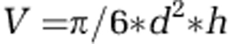where h is the largest cell dimension and d is the largest cross-section of h. We then used the equation of Menden-Deuer and Lessard (2000) to convert cell biovolume to cell biomass:

Within each sample, average cell biomass times cell abundance counted by TSA-FISH resulted in the total biomass of the HP assemblage.

FC counts

For protists, 4.8 ml of seawater were fixed with 25% glutaraldehyde EM grade (1% final concentration), deep frozen in liquid nitrogen and stored at −80 °C until analyzed in the laboratory within 7 months after the end of the cruise. Samples were processed with a FACSCalibur flow cytometer (BD Biosciences, San Jose, CA, USA) with a blue laser emitting at 488 nm using the settings described by Christaki et al. (2011) adapted from the protocol of Zubkov et al. (2007). Each sample was stained for at least 10 min in the dark with DMSO-diluted SYBRGreen I (Molecular Probes, Invitrogen, Paisley, UK) at a final concentration of 1:10 000. The flow rate was established at about 250 μl min⁻¹, with data acquisition for 5–8 min depending on cell abundance. Samples showing more than 1200 events s⁻¹ were diluted. Filtered samples (i.e., blanks) never had any event in the flow cytometrically defined area of interest. The flow cytometer output was analyzed using CellQuest software (Becton Dickinson, Franklin Lakes, NJ, USA), initially visualized as a cloud of points in a window showing side scatter (SSC) versus green fluorescence (FL1), which contained all cells stained by SYBR Green I. From this plot, target cells were identified after excluding the remaining noise, autofluorescent particles and heterotrophic prokaryotes, using different displays of the optical properties of the detected particles, as explained in Christaki et al. (2011). Measures were repeated several times in three random stations and the calculated standard errors corresponded to ∼1.5% of the average.

For heterotrophic prokaryotes, 1.2 ml of seawater were fixed with a paraformaldehyde–glutaraldehyde mix (1% and 0.05% final concentrations, respectively) and stored as described before for protists. Samples were stained with SYBRGreen I, at a final concentration of 1:10 000, for 15 min in the dark at room temperature. The flow rate ranged between 35 μl min⁻¹ (low) for samples above 1000 m depth and 150 μl min⁻¹ (high) for deeper samples. Acquisition time ranged from 30 to 260 s depending on cell concentration in each sample. Data were collected in a FL1 versus SSC plot and analyzed as detailed in Gasol and del Giorgio (2000). Molecular Probes latex beads (1 μm) were always used as internal standards.

For viruses, 1.2 ml of seawater were fixed with glutaraldehyde (0.5% final concentration) and stored as described above. The samples were stained with SYBRGreen I, and run at a medium flow speed after being diluted with TE buffer (1 × Tris-ethylenediaminetetraacetic acid) such that the event rate was between 100 and 800 viruses s⁻¹ (Marie et al., 1999). The data observed in the FL1 versus SSC plots were analyzed to select only the high DNA-content viruses (large viruses) from the total pool of viral particles as detailed elsewhere (Brussaard, 2004).

The cell biovolume of the prokaryotes was estimated using the calibration obtained by Calvo-Díaz et al. (2008) for oceanic samples, which relates relative side scatter (population SSC divided by bead SSC) to cell size. We used the same beads as in that study. Cell biovolume was converted to cell biomass with the equation of Gundersen et al. (2002):

Results

Optimizing the enumeration of HP by FC

We selected 10 stations well distributed along the Malaspina cruise (numbered in Figure 1) to compare counts of HP by FC with those obtained by the time-consuming but presumably more accurate epifluorescence microscopy. The standard counting approach based on DAPI staining has the advantage that it allows discrimination between the nucleus and cytoplasm and often displays the presence of flagella, making the identification more accurate. On the other hand, TSA-FISH specifically targets protists (those cells having eukaryotic ribosomes), and large bacteria are not confounded. Therefore, it was chosen as a second standard counting method to test and improve FC counts. Both microscopic counts provided very similar results (Figure 2a), with a linear slope of 1.02±0.07, not significantly different from 1 (P<0.0001; n=48; intercept=7.49) and an R² of 0.83.

Figure 2.

Methodologic comparison of deep ocean HP counts. (a) TSA-FISH counts versus DAPI counts and (b) TSA-FISH versus FC counts in samples from 10 selected vertical profiles (shown as numbered stations in Figure 1). Samples in panel b used to position the FC window are encircled by a light gray area. Regression lines are shown.

In FC counts, the accurate estimation of HP cells depends on how they are discriminated from heterotrophic prokaryotes in the cytograms, as both cell types are similarly labeled and share the same fluorescent properties (while they differ in size). For different depth ranges (200–450, 451–700, 701–1400 and 1401–4000) in three stations (40, 73 and 124), we identified the cytogram gate that displayed the best agreement between FC and TSA-FISH counts (linear slope of 0.81±0.09, P<0.0001; R² of 0.91; n=15; intercept=6.26; light gray dots in Figure 2b). Based on this gate positioning, other seven vertical profiles, for which we had TSA-FISH data, were analyzed and we obtained a very strong relationship between both counting methods in the 10 stations (linear slope of 0.83±0.07, P<0.0001; R² of 0.82; n=48; intercept=6.26; Figure 2b). These FC settings were subsequently applied to the vertical profiles of the other 55 stations (large dots in Figure 1) and to the deepest sample of the remaining stations (small dots in Figure 1).

Altogether, we estimated the abundance of deep HP in 71 vertical profiles combining the information obtained by microscopy and FC (10 profiles by the three methods, 55 profiles by FC and 6 profiles by TSA-FISH (in stations with abnormally high FC counts)) and in the deepest sample of 45 additional stations. In total, we estimated HP abundance in 476 individual samples.

Abundance and distribution of HP

The average (±s.e.) abundance of HP in the top layer of the mesopelagic region (200–450 m) was 72±19 cells ml⁻¹. This value doubled the bathypelagic concentration (32±3 cells ml⁻¹) and was more than six times greater than the 11±1 cells ml⁻¹ found in the deepest layer (1401–4000 m) (Table 1). Indeed, HP abundance decreased with depth as described by a log–log abundance versus depth slope of −0.68±0.04 and an R² of 0.61 (P<0.0001; Figure 3). We did not detect significant differences in the abundance-depth slopes among the three oceans considered (slopes of −0.70±0.04 in the Atlantic, −0.66±0.05 in the Indian and −0.66±0.06 in the Pacific Ocean).

Table 1. A global view of microbial components (protists, prokaryotes and large viruses) in the deep ocean.

Depth (m)	Heterotrophic protists			Prokaryotes		Large viruses
	Abundance (cells ml−1)	Biovolume (μm3 cell−1)	Biomass (pg C ml−1)	Abundance (105 cells ml−1)	Biomass (pg C ml−1)	Abundance (105 particles ml−1)
200–450	72±19	21±3	280±46	2.15±0.26	837±152	2.08±0.39
451–700	70±10	26±3	150±23	1.44±0.09	661±160	1.76±0.59
701–1400	32±3	33±6	112±28	0.98±0.07	534±106	0.89±0.17
1401–4000	11±1	48±9	50±14	0.56±0.08	309±59	0.42±0.05

The table shows the average values and s.e. for abundance, cell biovolume and community biomass in four different depth layers. Values of abundance are referred to 71 vertical profiles, whereas values of biovolume and biomass derive only from 6 vertical profiles.

Figure 3.

Abundance of HP versus depth in a log–log plot including all counts from this global study.

The highest HP abundance in both the mesopelagic and bathypelagic layers was found in the Equatorial Pacific (average±s.e.=101±38 and 20±2 cells ml⁻¹, respectively) (Table 2), exceeding that in the three Atlantic regions and North Pacific Oceans (P<0.05) and that in the North Pacific, Atlantic regions and Indian Oceans (analysis of variance, P<0.05), respectively (Figure 4). HP abundance at the deepest samples (ca. 4000 m) ranged between 1 and 58 cells ml⁻¹, and 75% of the counts were below 11 cells ml⁻¹ (n=116; Supplementary Figure S1). As shown before, most samples from the Equatorial Pacific were above this value. Owing to the potential overlap between large prokaryotes and small protists in FC analyses, these samples were recounted by TSA-FISH microscopy, which supported the generally higher HP abundances in this oceanic region.

Table 2. Microbial abundances of HP and PROK (and the ratio between both estimates) in the seven oceanic regions.

Region	Stations		HP abundance (cells ml−1)	Prokaryotic abundance (105 cells ml−1)	Ratio PROK:HP
EA	1–26	Total	29±3	0.91±0.09	3956±414
		Meso	43±3	1.33±0.10	3217±518
		Bathy	12±2	0.40±0.05	4866±864
SA	27–41	Total	25±3	0.46±0.06	1950±151
		Meso	38±4	0.71±0.09	2064±247
		Bathy	14±2	0.24±0.03	1848±185
IN	45–68	Total	32±4	1.09±0.10	4680±558
		Meso	52±7	1.54±0.10	3391±219
		Bathy	13±2	0.67±0.12	5930±1039
AB	69–78	Total	34±4	1.45±0.16	6135±1081
		Meso	53±4	2.21±0.15	4305±184
		Bathy	13±3	0.64±0.09	8073±2149
EP	81–98	Total	69±23	1.33±0.17	4109±807
		Meso	101±38	1.39±0.18	2762±484
		Bathy	20±2	1.24±0.31	6263±1854
NP	101–126	Total	30±4	1.79±0.34	6097±662
		Meso	43±6	2.31±0.45	5486±927
		Bathy	9±1	1.00±0.49	6844±937
NA	127–146	Total	43±13	0.58±0.06	3055±406
		Meso	80±28	0.94±0.09	2346±228
		Bathy	15±3	0.30±0.02	3603±688
Global	1–146	Total	34±3	0.99±0.05	4251±237
		Meso	54±5	1.44±0.06	3371±175
		Bathy	14±1	0.51±0.04	5177±439

Abbreviations: AB, Great Australian Bight; EA, Equatorial Atlantic; EP, Equatorial Pacific; HP, heterotrophic protest; IN, Indian; NA, North Atlantic; NP, North Pacific; PROK, prokaryotes; SA, South Atlantic.

The table shows the average values and s.e. in the total deep region or in the mesopelagic and bathypelagic layers.

Figure 4.

Abundance of HP with depth along the entire cruise visualized with ODV (ocean data view; Schiltzer, 2013). The track is separated in the oceanic regions indicated in Figure 1 (the departure and arrival harbor, Cadiz, appear in the middle of the plot only for graphical reasons). Small dots indicate sampling points.

Using the surface area for Atlantic, Pacific and Indian Oceans, we calculated an approximate volume (in 10⁶ km³) for mesopelagic (66, 133 and 59, respectively) and bathypelagic layers (247, 497 and 221, respectively). Using these volume estimates and mean cell abundance, we calculated a gross global number of cells for each ocean. Thus, for the mesopelagic layer, we found 7 × 10²⁴ cells in the Pacific, 4 × 10²⁴ in the Atlantic and 3 × 10²⁴ in the Indian Oceans. For the bathypelagic layer, the Pacific and Indian oceans harbored the same amount of cells than the mesopelagic waters, whereas for the Atlantic Ocean the number of HP estimated was 3 × 10²⁴ cells.

Main factors structuring HP abundance

We explored the possibility of predicting HP abundance with a multiple regression model using several abiotic parameters, such as depth, temperature, oxygen and salinity, and two biotic variables, such as prokaryote and large viruses abundances. After the first explorative analysis, we maintained only the three parameters that showed significance (P<0.05): depth, oxygen and prokaryote abundance. Repeating the analysis with these variables only, they had a very strong effect on HP abundance, with a significance of P<0.0001 for depth and prokaryotic abundance and P<0.001 for oxygen. The entire model explained 66% of the variability. Looking at the β-coefficient of each variable, which represents their relative potential at predicting HP, depth had the highest weight (β=0.61), followed by prokaryote abundance (0.28) and oxygen concentration (0.08).

The ratio between prokaryotes and HP abundances averaged 4251±237 in the global dark ocean (Table 2). This ratio was lower in the mesopelagic region (3364±174) than in the bathypelagic region (5195±441). There were significant differences between oceans (Table 2), with minimal ratios in the South Atlantic (1848±185) and maximal ratios in the Great Australian Bight (8073±2149). The abundance of HP increased as the 0.85±0.05 power of prokaryote abundance (R²=0.50, P<0.001; Figure 5). However, this pattern varied in each particular oceanic region, with slopes ranging from 0.77±0.10 in the South Atlantic to 1.28±0.13 in the North Atlantic (Table 3). Again, the Equatorial Pacific was unusual, as the relationship between prokaryote and HP abundances in that ocean was not significant (P=0.08).

Figure 5.

Abundance of HP versus prokaryote abundance in samples deriving from 71 vertical profiles.

Table 3. Slopes of the log–log relationships between the abundances of PROKs and HP, with additional statistics, for each oceanic region.

Region	Slope	P-value	R2
EA	1.05±0.08	0.0001	0.75
SA	0.77±0.10	0.0001	0.64
IN	1.16±0.10	0.0001	0.69
AB	1.14±0.12	0.0001	0.74
EP	0.33±0.18	0.0757	0.08
NP	0.95±0.12	0.0001	0.61
NA	1.28±0.14	0.0001	0.62

Abbreviations: AB, Great Australian Bight; EA, Equatorial Atlantic; EP, Equatorial Pacific; HP, heterotrophic protest; IN, Indian; NA, North Atlantic; NP, North Pacific; PROK, prokaryotes; SA, South Atlantic.

Cell size and biomass estimations

In seven selected stations (24, 34, 60, 73, 83, 102 and 133), we measured the size of individual cells by analyzing TSA-FISH microscopic images in all samples of the vertical profile. No clear differences were seen among the vertical profiles, and here we present the pooled data. We calculated the average cell biovolume of HP in the same depth layers defined before (Table 1). HP cells in the upper layer were significantly smaller (mean cell biovolume 21 μm³) than in the deeper layer (mean cell biovolume 48 μm³, P=0.004; Student's t-test). Within the cell size spectra, the most frequent classes were 10 and 15 μm³ (Figures 6a and b). The number of very small cells (equivalent diameter <3 μm) decreased with depth. Thus, 75% of cells in the 200–450 m layer were below this size threshold, whereas the contribution of very small cells was 62%, 57% and 54% in the consecutive depth layers.

Figure 6.

(a) Biovolume spectra of HP cells in different depth layers. Each class takes the name of its higher value (e.g. class 10 comprises cells from 5.01 to 10 μm³), except the last class, where all the cells with a biovolume >35 μm³ were pooled together. The equivalence of cell biovolume to equivalent spherical diameter is also indicated in the top bar. (b) Some micrographs of bathypelagic HP cells, showing different cell shapes and the presence of flagella. The blue signal corresponds to the DAPI-stained nucleus and the green signal to the TSA-FISH-stained cytoplasm. Split morphotypes are shown in pictures 1 and 2.

HP biomass ranged broadly from 4 to 486 pg C ml⁻¹ (Supplementary Figure S2a), with an average of 280±46 pg C ml⁻¹ in the upper 200–450 m layer, and a subsequent reduction of HP biomass in the three following layers: 150±23, 112±28 and 50±14 pg C ml⁻¹ (Table 1). Three bathypelagic samples in the North Pacific at 2000 m, the Great Australian Bight at 2800 m and the Indian Ocean at 4000 m showed deviating high values of 146, 175 and 90 pg C ml⁻¹, respectively. In the last two cases, the higher biomass values were because of larger cell sizes and not because of higher abundances.

The biomass of prokaryotes in the same seven vertical profiles also decreased with depth, but the decrease was less pronounced than that of HP biomass (Supplementary Figure S2b). The slopes of the log–log plot were −0.53 for HP biomass and −0.75 for prokaryotes, and they were significantly different (P<0.0001, analysis of covariance). Consequently, the log–log plot of prokaryotic versus HP biomass using all samples revealed a nonsignificant relationship (P=0.09). However, this relationship becomes significant when removing station 73 (with anomalous high biomass) from the analysis (n=29, slope of 0.84, P=0.01, R²=0.22). The global ratio between eukaryotic and prokaryotic biomass was 0.30 (±5), being 0.39 for the mesopelagic and 0.21 for the bathypelagic.

Discussion

The unprecedented magnitude of our sampling effort (116 stations) and the geographical coverage in our study (Figure 1) allowed for a first global assessment of the abundance of HP in mesopelagic and bathypelagic waters of the world's main oceans. Compared with the research carried out on deep prokaryotes, only a handful of studies have enumerated deep HP (Pomeroy and Johannes, 1968; Sorokin, 1985; Tanaka and Rassoulzadegan, 2002; Yamaguchi et al., 2004; Fukuda et al., 2007; Sohrin et al., 2010; Morgan-Smith et al., 2011, 2013), likely because of the time-consuming enumeration techniques required. Here we used FC to estimate the abundance of HP (Christaki et al., 2011), a routine that had not yet been used in large-scale oeanographic surveys. In parallel, we used microscopy in selected samples to test for the accuracy of FC, verify FC counts and exclude unrealistic values. Deep HP visualized in DAPI-stained preparations included several cell shapes and the presence of flagella, but sometimes their identification was doubtful. This led us to use the TSA-FISH technique with a probe targeting all eukaryotic cells to complement the general DAPI staining. The agreement between the two methods (epifluorescence and FC) was strong (Figure 2). Coupling techniques combining the speed of automatic enumeration with the accuracy of direct observations is strongly recommended in case of a large number of samples as typically derived from oceanographic cruises, although the 7-month duration of the Malaspina Expedition far exceeds the duration and sampling effort of most campaigns.

In general, the HP abundances observed in the bathypelagic layer (ca. 1–15 cells ml⁻¹) were in the same range cited in previous reports (Tanaka and Rassoulzadegan, 2002; Fukuda et al., 2007; Boras et al., 2010; Sohrin et al., 2010; Morgan-Smith et al., 2013). However, along the entire expedition we found several sites with exceptionally higher abundances, particularly in the South Pacific. At the global level, the abundance of HP decreased with the −0.68±0.04 power of depth from 72 cells ml⁻¹ in the upper mesopelagic layer to 11 cells ml⁻¹ at the lower bathypelagic layer, very close to the −0.66 power reported earlier for a smaller data set from Atlantic and Pacific samples (Arístegui et al., 2009). Despite the global trend of decreasing abundance with depth, the distribution of HP cells was not equal at the same depth range over the analyzed transect (Figure 4). This ocean basin variation in HP abundance was mostly related, among the considered parameters, to prokaryote abundance. Considering that some authors suggested a possible control by large viruses specifically on protistan populations (Wommack et al., 1999; Steward et al., 2000), we also tested the importance of large viruses on HP abundance. In the multiple regression model, this relation had no significance, and thus a clear effect of large viruses on HP was not detected in the deep ocean. Epifluorescence microscopic inspections allowed identification of most of the cell shapes defined by Morgan-Smith et al. (2011, 2013). Although counting and classifying according to cell shapes was not the aim of our study, we noticed that the ‘split morphotype' (with no clear taxonomic assignation), which was the most abundant morphotype in that study, was almost ubiquitous in Malaspina bathypelagic samples (Figure 6b, see pictures 1 and 2). Many of the microscopically observed cells showed flagella (Figure 6b), so potentially part of these cells could be active grazers (Jürgens and Massana, 2008). With respect to the mean size, deep protists tended to be slightly larger than surface ocean ones. Indeed, 54% of the bathypelagic protists had a biovolume between 5 and 15 μm³ (Figure 6a) corresponding to spherical equivalent diameters of 2–3 μm, whereas this size range represents about 76% in surface waters (Jürgens and Massana, 2008). The mean cell biovolume tended to increase with depth, in contrasts with Fukuda et al. (2007), who found a decrease in the contribution of larger cells with depth in the subarctic Pacific. The absence of deformed or exploded cells during the microscopic counts led us to exclude the effects of volume enlargement due to decompression.

The estimations of HP community biomass were carried out in one vertical profile per oceanic region. As expected, at a global level, HP biomass decreased clearly with depth, from 280 pg C ml⁻¹ in the upper mesopelagic layer to 50 pg C ml⁻¹ in the lower bathypelagic layer. The average biomass for the bathypelagic realm was one order of magnitude larger than the values estimated by Fukuda et al. (2007) and Sohrin et al. (2010) but similar to other reports (Tanaka and Rassoulzadegan, 2002; Yamaguchi et al., 2004). The biomass ratio between HP and prokaryotes was 0.21±0.05 in the global bathypelagic realm and 0.39±0.08 in the mesopelagic realm. This is reflected by a faster decrease of HP biomass than prokaryote biomass with depth (power slopes of −0.53 and −0.75, respectively). The excess of prokaryotic biomass (as compared with HP biomass) leaves open the question about the importance of the HP grazing pressure on prokaryotes in the deeper bathypelagic ocean.

The impact of grazing on prokaryotes in the deep ocean is a matter of debate (Fukuda et al., 2007; Arístegui et al., 2009; Boras et al., 2010; Nagata et al., 2010), and interesting clues can derive from analyzing the ratio in the abundance of prokaryotes and HP cells (PROK:HP ratio). Considering the bathypelagic region globally, there were 5195±441 prokaryotic cells for each protist. This is three times the ratio found in an epipelagic reference data set, 1760±162 (averaged data from the following papers: Kirchman et al., 1989; Cho et al., 2000; Tanaka and Rassoulzadegan, 2002; Yamaguchi et al., 2002, 2004; Tanaka et al., 2005), indicating less protists for a given prokaryote cell in deep waters than at surface. A putative reason for the higher PROK:HP ratio in deep waters would be that the prokaryote abundance in the deep ocean is below the numerical threshold of grazing (Andersen and Fenchel, 1985), thus protists spend a lot of energy (via respiration) in the search for prey and as a result prokaryotes are inefficiently grazed. Alternatively, HP cells could be sustained at low prokaryotic abundances given the micropatch distribution theory (Simon et al., 2002; Baltar et al., 2009) that suggests that most of the interactions between HP and prokaryotes take place in large or small aggregates where prey density is high enough to sustain HP growth.

Interestingly, this ratio displays a substantial variability at local scale. For instance, the Atlantic community is characterized by a low ratio with no significant difference between mesopelagic and bathypelagic regions, whereas the bathypelagic layer of the Great Australian Bight exhibited the highest ratios (8073±2149). This variability could be owing to the fact that the counted HP cells belong not only to grazers but also to osmotrophs or parasites that are independent from prokaryotic abundance. In fact, some cells could belong to unicellular fungi, known to be unable to perform phagocytosys because of their chitin cell wall (Richards et al., 2012). In a parallel study of the diversity of deep microeukaryotes by pyrosequencing 18S rDNA genes, we estimated the contribution of fungal sequences in 25 samples (Pernice et al., in preparation), and therefore could use the presence of fungal signal to explain the ratio variability in the deep ocean. In general, areas with higher PROK:HP ratios, such as the Pacific, showed a larger contribution of fungi. The relationship between the PROK:HP ratio and the fungal contribution (Figure 7) was very significant (n=25, P=0.0005, R²=0.4). The presence of fungi within deep HP assemblages would mean that prokaryotes are not the only carbon source for HP. The fact that some of the HP counted could be osmotrophs or parasites instead of prokaryote grazers would result in a certain relaxation of the grazing pressure on prokaryotes, thus deriving in higher PROK:HP ratios. The good relationship shown in Figure 7 supports the hypothesis that high PROK:HP ratios may be explained by the presence of trophic strategies alternative to grazing.

Figure 7.

Relationship of the abundance ratio of prokaryotes and HP cells with respect the percentage of fungi sequences in the corresponding samples. The latter values derive from a parallel study on deep ocean protist diversity (Pernice et al., in preparation).

In summary, this study confirms and extends previous results on HP distribution in the deep ocean, and provides a more comprehensive global view. Our wide sampling coverage showed that HP were ubiquitous, with minimal abundances of around 10 cells ml⁻¹, and that their biomass averaged approximately 20% of prokaryote biomass in the global bathypelagic realm, with this ratio increasing at depth as HP biomass declines faster with depth than prokaryote biomass does. The maintenance of this microeukaryotic biomass likely requires active grazing on prokaryotes and the presence of osmotrophic nutrition and parasitism. Our work suggests that HP should be considered important players in the dark ocean and highlights the importance of studying the dynamics and diversity of this microbial food web component.

The authors declare no conflict of interest.

References

- Andersen P, Fenchel T. Bacterivory by microheterotrophic flagellates in seawater samples. Limnol Oceanogr. 1985;30:198–202. [Google Scholar]
- Arístegui J, Duarte CM, Gasol JM, Herndl GJ. Microbial oceanography of the dark ocean's pelagic realm. Limnol Oceanogr. 2009;54:1501–1529. [Google Scholar]
- Baltar F, Arístegui J, Sintes E, Van Aken HM, Gasol JM, Herndl GJ. Evidence of prokaryotic metabolism on suspended particulate organic matter in the dark waters of the subtropical North Atlantic. Limnol Oceanogr. 2009;54:182–193. [Google Scholar]
- Boras JA, Sala MM, Baltar F, Arístegui J, Duarte CM, Vaqué D. Effect of viruses and protists on bacteria in eddies of the Canary Current region (subtropical northeast Atlantic) Limnol Oceanogr. 2010;55:885–898. [Google Scholar]
- Brussaard CPD. Optimization of procedures for counting viruses by flow cytometry. Appl Environ Microbiol. 2004;70:1506–1513. doi: 10.1128/AEM.70.3.1506-1513.2004. [DOI] [PMC free article] [PubMed] [Google Scholar]
- Calvo-Díaz A, Morán XAG, Suárez LÁ. Seasonality of picophytoplankton chlorophyll a and biomass in the central Cantabrian Sea, southern Bay of Biscay. J Mar Syst. 2008;72:271–281. [Google Scholar]
- Cho BC, Na SC, Choi DH. Active ingestion of fluorescently labelled bacteria by mesopelagic heterotrophic nanoflagellates in the East Sea, Korea. Mar Ecol Prog Ser. 2000;206:23–32. [Google Scholar]
- Christaki U, Courties C, Massana R, Catalá P, Lebaron P, Gasol JM, et al. Optimized routine flow cytometric enumeration of heterotrophic flagellates using SYBR Green I. Limnol Oceanogr. 2011;9:329–339. [Google Scholar]
- Dick GJ, Anantharaman K, Baker BJ, Li M, Reed DC, Sheik CS. The microbiology of deep-sea hydrothermal vent plumes: ecological and biogeographic linkages to seafloor and water column habitats. Front Microbiol. 2013;4:124. doi: 10.3389/fmicb.2013.00124. [DOI] [PMC free article] [PubMed] [Google Scholar]
- Fukuda H, Sohrin R, Nagata T, Koike I. Size distribution and biomass of nanoflagellates in meso- and bathypelagic layers of the subarctic Pacific. Aquat Microb Ecol. 2007;46:203–207. [Google Scholar]
- Gasol JM, Alonso-Sáez L, Vaqué D, Baltar F, Calleja ML, Duarte CM, et al. Mesopelagic prokaryotic bulk and single-cell heterotrophic activity and community composition in the NW Africa–Canary Islands coastal-transition zone. Prog Oceanogr. 2009;83:189–196. [Google Scholar]
- Gasol JM, del Giorgio PA. Using flow cytometry for counting natural planktonic bacteria and understanding the structure of planktonic bacterial communities. Sci Mar. 2000;64:197–224. [Google Scholar]
- Gundersen K, Heldal M, Norland S, Purdie DA, Knap AH. Elemental C, N, and P cell content of individual bacteria bollected at the Bermuda Atlantic Time-Series Study (BATS) Site. Limnol Oceanogr. 2002;47:1525–1530. [Google Scholar]
- Hillebrand H, Dürselen C-D, Kirschtel D, Pollingher U, Zohary T. Biovolume calculation for pelagic and benthic microalgae. J Phycol. 1999;35:403–424. [Google Scholar]
- Jiao N, Zheng Q. The microbial carbon pump: from genes to ecosystems. Appl Environ Microbiol. 2011;77:7439–7444. doi: 10.1128/AEM.05640-11. [DOI] [PMC free article] [PubMed] [Google Scholar]
- Jürgens K, Massana R.2008Protistan grazing on marine bacterioplanktonIn: Kirchman DL (ed)Microbial Ecology of the Oceans2nd ednWiley: New York, NY, USA; 383–441. [Google Scholar]
- Kirchman DL, Keil RG, Wheeler PA. The effect of amino acids on ammonium utilization and regeneration by heterotrophic bacteria in the subarctic Pacific. Deep-Sea Res. 1989;36:1763–1776. [Google Scholar]
- Lim EL, Dennet MR, Caron DA. The ecology of Paraphysomonas imperforata based on studies employing oligonucleotide probe identification in coastal water samples and enrichment cultures. Limnol Oceanogr. 1999;44:37–51. [Google Scholar]
- Marie D, Brussaard CPD, Thyrhaug R, Bratbak G, Vaulot D. Enumeration of marine viruses in culture and natural samples by flow cytometry. Appl Environ Microbiol. 1999;65:45–52. doi: 10.1128/aem.65.1.45-52.1999. [DOI] [PMC free article] [PubMed] [Google Scholar]
- Marie D, Simon N, Vaulot D.2005Phytoplankton cell counting by flow cytometryIn: Andersen RA (ed)Algal Culturing Techniques Academic Press: New York, NY, USA; 253–267. [Google Scholar]
- Massana R, Terrado R, Forn I, Lovejoy C, Pedrós-Alió C. Distribution and abundance of uncultured heterotrophic flagellates in the world oceans. Environ Microbiol. 2006;8:1515–1522. doi: 10.1111/j.1462-2920.2006.01042.x. [DOI] [PubMed] [Google Scholar]
- Menden-Deuer S, Lessard EJ. Carbon to volume relationship for dinoflagellates, diatoms and other protist plankton. Limnol Oceanogr. 2000;45:569–579. [Google Scholar]
- Morgan-Smith D, Clouse MA, Herndl GJ, Bochdansky AB. Diversity and distribution of microbial eukaryotes in the deep tropical and subtropical North Atlantic Ocean. Deep-Sea Res Part I. 2013;78:58–69. [Google Scholar]
- Morgan-Smith D, Herndl GJ, van Aken HM, Bochdansky AB. Abundance of eukaryotic microbes in the deep subtropical North Atlantic. Aquat Microb Ecol. 2011;65:103–115. [Google Scholar]
- Nagata T, Tamburini C, Arístegui J, Baltar F, Bochdansky AB, Fonda-Umani S, et al. Emerging concepts on microbial processes in the bathypelagic ocean—ecology, biogeochemistry, and genomics. Deep-Sea Res Part II. 2010;57:1519–1536. [Google Scholar]
- Pernthaler J, Glöckner F, Schönhuber W, Amann R. Fluorescence in situ hybridization (FISH) with rRNA-targeted oligonucleotide probes. Method Microbiol. 2001;30:207–226. [Google Scholar]
- Pomeroy LR, Johannes RE. Respiration of ultraplankton in the upper 500 meters of the ocean. Deep-Sea Res. 1968;15:381–391. [Google Scholar]
- Porter K, Feig Y. The use of DAPI for identifying and counting aquatic microflora. Limnol Oceanogr. 1980;25:943–948. [Google Scholar]
- Richards TA, Jones MDM, Leonard G, Bass D. Marine fungi: their ecology and molecular diversity. Ann Rev Mar Sci. 2012;4:495–522. doi: 10.1146/annurev-marine-120710-100802. [DOI] [PubMed] [Google Scholar]
- Schiltzer R.2013. Ocean Data View. Available at: : http://odv.awi.de (accessed 13 June 2012).
- Simon M, Grossart H-P, Schweitzer B, Ploug H. Microbial ecology of organic aggregates in aquatic ecosystems. Aquat Microb Ecol. 2002;28:175–211. [Google Scholar]
- Sohrin R, Imazawa M, Fukuda H, Suzuki Y. Full-depth profiles of prokaryotes, heterotrophic nanoflagellates, and ciliates along a transect from the equatorial to the subarctic central Pacific Ocean. Deep-Sea Res Part II. 2010;57:1537–1550. [Google Scholar]
- Sorokin YI. Phosphorus metabolism in planktonic communities of the Eastern Tropical Pacific. Mar Ecol Prog Ser. 1985;27:87–97. [Google Scholar]
- Steward GF, Montiel JL, Azam F. Genome size distributions indicate variability and similarities among marine viral assemblages from diverse environments. Limnol Oceanogr. 2000;45:1697–1709. [Google Scholar]
- Tanaka T, Rassoulzadegan F. Full-depth profile (0–2000 m) of bacteria, heterotrophic nanoflagellates and ciliates in the NW Mediterranean Sea: vertical partitioning of microbial trophic structures. Deep-Sea Res Part II. 2002;49:2093–2107. [Google Scholar]
- Tanaka T, Rassoulzadegan F, Thingstad TF. Analyzing the trophic link between the mesopelagic microbial loop and zooplankton from observed depth profiles of bacteria and protozoa. Biogeosciences. 2005;2:9–13. [Google Scholar]
- Wommack EK, Ravel J, Hill RT, Chun J, Colwell RR. Population dynamics of Chesapeake Bay virioplankton: total-community analysis by pulse-field gel electrophoresis. Appl Environ Microbiol. 1999;65:231–240. doi: 10.1128/aem.65.1.231-240.1999. [DOI] [PMC free article] [PubMed] [Google Scholar]
- Yamaguchi A, Watanabe Y, Ishida H, Harimoto T, Furusawa K, Suzuki S, et al. Structure and size distribution of plankton communities down to the greater depths in the western North Pacific Ocean. Deep-Sea Res Part II. 2002;49:5513–5529. [Google Scholar]
- Yamaguchi A, Watanabe Y, Ishida H, Harimoto T, Furusawa K, Suzuki S, et al. Latitudinal differences in the planktonic biomass and community structure down to the greater depths in the western north Pacific. J Oceanogr. 2004;60:773–787. [Google Scholar]
- Zubkov MV, Burkill PH. Syringe pumped high speed flow cytometry of oceanic phytoplankton. Cytometry Part A. 2006;69A:1010–1019. doi: 10.1002/cyto.a.20332. [DOI] [PubMed] [Google Scholar]
- Zubkov MV, Burkill PH, Topping JN. Flow cytometric enumeration of DNA-stained oceanic planktonic protists. J Plankton Res. 2007;29:79–86. [Google Scholar]
Associated Data
This section collects any data citations, data availability statements, or supplementary materials included in this article.