Economic Choices Reveal Probability Distortion in Macaque Monkeys

Abstract

Economic choices are largely determined by two principal elements, reward value (utility) and probability. Although nonlinear utility functions have been acknowledged for centuries, nonlinear probability weighting (probability distortion) was only recently recognized as a ubiquitous aspect of real-world choice behavior. Even when outcome probabilities are known and acknowledged, human decision makers often overweight low probability outcomes and underweight high probability outcomes. Whereas recent studies measured utility functions and their corresponding neural correlates in monkeys, it is not known whether monkeys distort probability in a manner similar to humans. Therefore, we investigated economic choices in macaque monkeys for evidence of probability distortion. We trained two monkeys to predict reward from probabilistic gambles with constant outcome values (0.5 ml or nothing). The probability of winning was conveyed using explicit visual cues (sector stimuli). Choices between the gambles revealed that the monkeys used the explicit probability information to make meaningful decisions. Using these cues, we measured probability distortion from choices between the gambles and safe rewards. Parametric modeling of the choices revealed classic probability weighting functions with inverted-S shape. Therefore, the animals overweighted low probability rewards and underweighted high probability rewards. Empirical investigation of the behavior verified that the choices were best explained by a combination of nonlinear value and nonlinear probability distortion. Together, these results suggest that probability distortion may reflect evolutionarily preserved neuronal processing.

Introduction

Economic choices between uncertain options require an appreciation of reward utility and a proper understanding of reward probability. Indeed, linear probability weighting is a central assumption in normative theories of risky decision making such as expected utility theory (von Neumann and Morgenstern, 1944). However, a well known paradox and many experimental studies have demonstrated that humans often overweight low probability outcomes and underweight high probability outcomes (Allais, 1953; Kahneman and Tversky, 1979; Prelec, 1998; Gonzalez and Wu, 1999; Abdellaoui, 2000; Tobler et al., 2008; Hsu et al., 2009). The Allais paradox illustrated that many decision makers would forego the chance of a large gain when the chance of getting nothing increased from 0 to 1/100; howeer, those same decision makers would choose the very same chance of a large gain when the chance of getting nothing increased from 89 to 90/100 (Allais, 1953). Therefore, a small increase in the probability of getting nothing appeared more significant at low probabilities compared with higher ones. This phenomenon, probability distortion, has subsequently been incorporated into modern decision theories (Kahneman and Tversky, 1979; Quiggin, 1982; Tversky and Kahneman, 1992) that provide a better description of human behavior compared with expected utility theory (Machina, 1987). However, it is not known whether probability distortion occurs in macaque monkeys, which afford excellent opportunities for studying neuronal mechanisms underlying economic choices.

Previous studies of decision making in monkeys have measured a diversity of risk attitudes, but none has identified probability distortions. The majority have shown that monkeys are risk seeking for small rewards (McCoy and Platt, 2005; O'Neill and Schultz, 2010; Kim et al., 2012; So and Stuphorn, 2012; Lak et al., 2014; Raghuraman and Padoa-Schioppa, 2014), but others have uncovered the risk aversion more commonly observed in humans (Yamada et al., 2013; Stauffer et al., 2014). In these studies, risk was modulated either by changing probability and magnitude (So and Stuphorn, 2012; Raghuraman and Padoa-Schioppa, 2014) or by holding probability constant and changing the magnitude (McCoy and Platt, 2005; Kim et al., 2012; Yamada et al., 2013; Lak et al., 2014; Stauffer et al., 2014). Therefore, there has been no systematic investigation of probability distortion in monkeys.

Here, we investigated whether monkeys exhibited a nonlinear probability weighting function independent from nonlinear utility. We constructed gambles with constant outcome utilities but different reward probabilities and observed value-based choices between these gambles and safe rewards. In this way, we measured the certainty equivalents (CEs) of these gambles, defined as the amount of reward for which the monkey is indifferent between receiving that amount of reward for certain and taking the gamble. We parametrically separated nonlinear probability weighting from nonlinear utility and followed this analysis with several empirical tests to validate the estimated functions. Our results revealed overweighting of small probability rewards and underweighting of high probability rewards. The one-parameter Prelec probability weighting function (Prelec, 1998) best explained the trial-by-trial choice behavior. Therefore, similar to humans, monkeys displayed an inverted S-shaped probability weighting function with a crossover point below p = 0.5.

Materials and Methods

Animals and experimental setup.

Two male rhesus monkeys (Macaca mulatta) were used for these studies (9.1 and 12.5 kg). A third subject (weighing 17 kg) was used for one test, shown in Figure 6. The Home Office of the United Kingdom approved all experimental protocols and procedures.

Figure 6.

Subjective values reflecting nonlinear utility and probability distortion. a, Animals preferred the riskier of two gambles with same mean and probability but different outcome magnitudes. Each bar represents the average CE for a 50:50 gamble between 0.1 and 0.4 ml (G1, gray) or a 50:50 gamble between 0 and 0.5 ml (G2, black). Gamble G2 is a mean preserving spread of gamble G1, so probability distortion cannot explain the preference, which is likely due to convex utility. Error bars are SEM across CE measurements (n = 16 in monkey B, 6 in monkey C). b, Utility functions fit to the CEs of the 50:50 gambles reflect the convex utility functions that were parametrically estimated from the choices (Fig. 4c,d). Light and dark gray lines and dots represent the fitted utility functions and mean CE from 50:50 gambles, respectively, from monkeys A and B, respectively. Error bars are SEM across CEs. Because the origin and scale of the utility axis are 0 and 1, the expected utility (EU) mirrors the indicated probability. The blue arrow illustrates this relationship for a gamble with a p = 0.25 chance of 0.5 ml or 0 otherwise. We projected the observed CE for the same gamble (orange arrow) onto the utility axis to estimate u(CE), which revealed the observed probability (p̂). c, Observed (p̂) is larger than indicated probability (p) at low indicated probabilities (positive difference, indicating overweighting), whereas observed (p̂) is smaller than indicated probability (p) at higher indicated probabilities (negative difference, indicating underweighting). The p̂ values were calculated separately for each animal (so that we could use the separate utility functions shown in b and avoid impossible interpersonal utility comparisons) and then combined. The black dots represent the average data in 13 equally populated bins (excluding 0 and 1 endpoints). Error bars are SEM across p̂ − p measurements. The green line represents the difference between the optimized one-parameter probability weighting function (averaged across the two animals) and the indicated probability. The secondary y-axis corresponds to the green line.

A custom-made head holder was aseptically implanted under general anesthesia before the experiment. During experiments, animals sat in a primate chair (Crist Instruments) positioned 30 cm from a computer monitor. Eye position was monitored noninvasively using infrared eye tracking (ETL200; ISCAN). Eye data and digital task event signals were sampled at 2 kHz and stored at 200 Hz (eye) or 1 kHz. Liquid reward was delivered by means of a computer-controlled solenoid liquid valve (0.004 ml/ms opening time). Custom-made software (MATLAB; The MathWorks) running on a Microsoft Windows XP computer controlled the behavioral tasks.

Behavioral training and tasks.

We first trained monkeys on reward predicting cues (see Fig. 1a). Following successful central gaze fixation for 0.5 s, one cue (pseudorandomly drawn) was presented on the screen for 1.5 s and the reward was delivered at cue offset. There was no further operant requirement after the central fixation time had ended and the cue appeared. Unsuccessful central fixation resulted in a 6 s timeout. The gamble cue (see Fig. 1b) was a pie chart with two sectors whose areas corresponded to the probability of reward (p, indicated by horizontal bars) and no reward (1−p, indicated by vertical bars), respectively. The safe cues (see Fig. 1c) contained one horizontal bar whose vertical position indicated the reward amount (between 0 and 0.8 ml in monkey A and between 0 and 1.2 ml in monkey B). Training was done in blocks for the two cue types, and included 3 safe and 6 gamble cues (p = 0.10, 0.25, 0.40, 0.60, 0.75 or 0.90 in both monkeys; > 4000 trials over a month in monkey A and 3900 trials over 3 weeks in monkey B). Within each block cues were presented to the monkey in pseudorandom order. Importantly, during training and the choice tasks (see Figs. 1d, 2a), the area indicating the probability of reward (horizontally striped sector) began at a pseudorandomly selected angle between 0 and 360 (theta(∅), see Fig. 1b). Therefore, the section indicating reward could appear on any part of the pie chart, insuring that animals evaluated the whole stimulus rather than only considering a particular portion associated with the reward.

Figure 1.

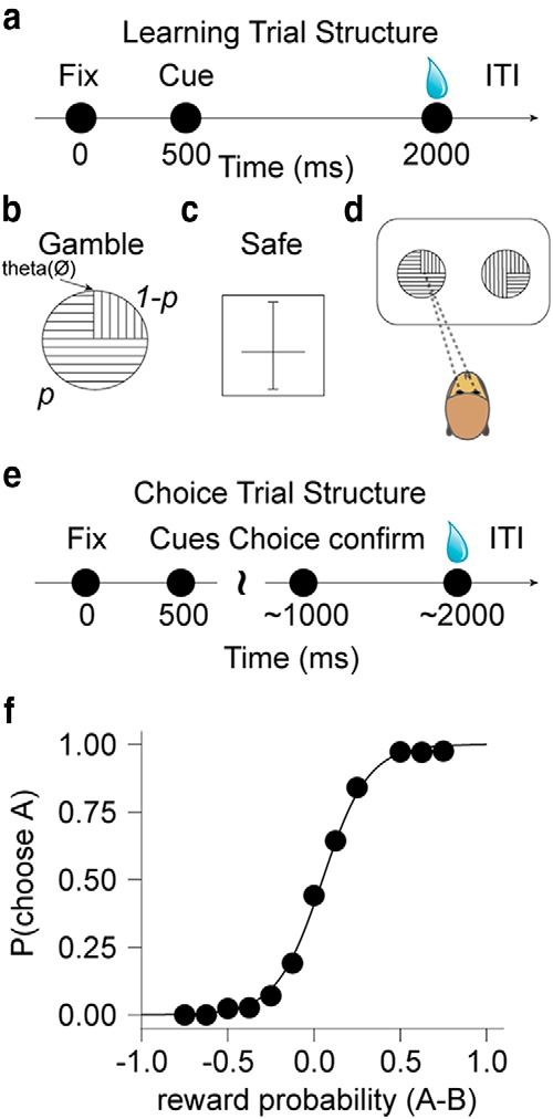
Behavioral training and choice task. a, Pavlovian trial structure. The animal had to fix its gaze on a central spot to start the trial, the cue was presented 0.5 s later, and the reward was delivered 1.5 s after cue onset. b, c, Cues indicating gambles and safe rewards. Gambles were indicated by a pie chart (b) with two sectors, indicated by horizontal and vertical lines, the areas of which corresponded to the probability of reward (0.5 ml) and no reward, respectively. θ corresponded to the starting angle of the rewarded probability sector (horizontal lines). On every trial, it was pseudorandomly selected (between 0 and 360) such that the rewarded sector could appear on any portion of the cue. Safe offers were indicated by a horizontal bar crossing a vertical scale (c) that represented volumes from 0 (bottom) to 0.8 ml (top) (1.2 ml in monkey B). d, Saccadic choices between two sector cues, each indicating a gamble. e, Saccade choice trial structure. The animal fixed its gaze on a central spot to start the trial, 2 cues were presented 0.5 s later, after which the animal had 1 s to indicate its choice with a saccade to 1 of the 2 cues. The unchosen target disappeared and the chosen option remained on the screen for 1 s, after which the reward was delivered. The timing of the choice trials approximated the timing of the Pavlovian learning trials. f, Probability of choosing one of the gambles as a function of difference in probability of the two presented gambles. Dots show average choice probability in 12 equally populated bins for monkey A. Black line is a logistic fit on the trial-by-trial data.

Figure 2.

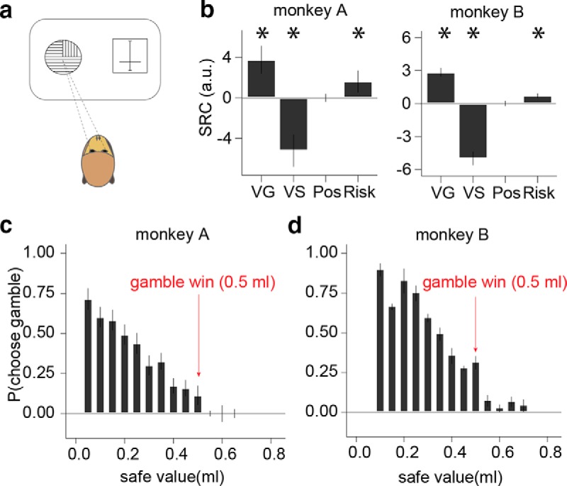
Explicit cue information used for choices. a, Choice task for measuring CEs and trial-by-trial choice data for probability distortion analysis. One gamble and one safe cue were presented on pseudorandomly alternating sides of the computer monitor and the animal indicated its choice by making a saccade to one of the cues. b, Standardized regression coefficients (SRCs) for choices between gambles and safe rewards. VG and VS, Value of the gamble and safe options, respectively; Pos, position on the screen; Risk, risk of the gamble. Error bars indicate SD of regression coefficients across sessions. Asterisks indicate significant regressors (VG: p = 5.02⁻¹⁰ and 9.44⁻¹²; VS: p = 7.94⁻¹² and 1.64⁻¹²; Risk: p = 4.62⁻⁶ and 6.22⁻⁸, all in monkeys A and B, respectively; t test). c, d, Choice probability versus safe offer value for low reward probability gambles (p < 0.3). Each bar represents the average likelihood for choosing the gamble at different safe offer values in 0.05 ml bins. Red arrow indicates the winning outcome magnitude of the gamble (0.5 ml). The animals rarely chose the gamble when the safe offer was >0.5 ml, providing strong evidence that they understood the value of cues relative to each other. Error bars are SEM across reward probability.

We assessed binary choices between different gambles (n = 2444 and 1101 trials in monkey A and B, respectively, see Fig. 1d), and between a gamble and a safe reward (n = 8885 and 4699 trials in monkey A and B, respectively, see Fig. 2a). Each trial (see Fig. 1e) began with a fixation spot at the center of the monitor. The animal directed its gaze to the fixation spot and held it there for 0.5 s. Following successful central fixation, the fixation spot disappeared and two gamble cues (see Fig. 1d), or one gamble cue and one safe cue (see Fig. 2a), were pseudorandomly selected and appeared to the left and right of the fixation spot, pseudorandomly varying between the two positions. The animal had 1 s to indicate its choice by shifting its gaze to the center of the chosen cue and holding it there for another 0.5 s. Then the unchosen cue disappeared while the chosen cue remained on the screen for an additional 1 s. The reward was delivered at offset of the chosen cue. Trials were interleaved with intertrial intervals of pseudorandom durations conforming to a truncated Poisson distribution (λ = 5, truncated at 2 and 8 s). Unsuccessful fixation during any task epoch resulted in a 6 s timeout.

Measurement of certainty equivalent using parameter estimation by sequential testing

To measure the certainty equivalent (CE) for different gambles, we used an adaptive psychometric measurement technique (Parameter Estimation by Sequential Testing, PEST) adapted from Luce (Luce, 2000) and fully described previously (Lak et al., 2014). Using this procedure we assessed the amount of blackcurrant juice that was subjectively equivalent to the value associated with each gamble. Each PEST sequence consisted of several consecutive trials during which one gamble was presented as a choice option against the safe reward. During each experimental session we performed 15 to 30 PEST procedures. During each individual PEST procedure (6–30 trials), the gamble was constant (i.e., it indicated a constant reward probability). Similar to initial learning task, theta(∅) was selected pseudorandomly on every trial throughout the PEST. During each daily session we pseudorandomly selected the tested probabilities such that the average probability for the daily session was ∼p = 0.5.

On the initial trial of a PEST sequence, the amount of safe reward was chosen pseudorandomly from the interval 0.1 to 0.8 ml (1.2 ml for monkey B). Based on the animal's choice between the safe reward and gamble, the safe amount was adjusted on the following trial. If the animal chose the gamble on trial t, then the safe amount was increased by ε on trial t + 1. However, if the animal chose the safe reward on trial t, the safe amount was reduced by ε on trial t+1. Initially, ε was large. After the third trial of a PEST sequence, ε was adjusted according to the doubling rule and the halving rule. Specifically, every time two consecutive choices were the same, the size of ε was doubled, and every time the animal switched from one option to the other, the size of ε was halved. Therefore, the procedure converged by locating subsequent safe offers on either side of the true indifference value and reducing ε until the interval containing the indifference value was small. The size of this interval is a parameter set by the experimenter, called the exit rule. For our study, the exit rule was 20 μl. When ε fell below the exit rule, the PEST procedure terminated, and the indifference value was calculated by taking the mean of the final two safe offers (see Lak et al., 2014 and Stauffer et al., 2014 for further details). A typical PEST session lasted 15–20 trials. All together, we collected 602 PEST measurements from monkey A over 8885 trials, and 278 PEST measurements over 4699 trials.

Behavioral analysis.

Trial-by-trial data was collected and stored for analysis in Matlab and R (Wickham, 2009; RCoreTeam, 2014). We analyzed two types of data: CEs collected by running PEST sequences (see above) and discrete trial-by-trial choice data.

We first verified the monkeys appropriately used the information provided by the sector cues during choices between two gambles, analyzed using logistic regression as follows:

where y was 1 when Gamble1 was chosen and 0 otherwise (error trials, which accounted for <5% of all trials, were not included in this analysis), V_Gamble1 and V_Gamble2 were determined by the probability of getting 0.5 ml in each gamble gamble, and position LR indicated the position on the screen.

Whereas choices between gamble cues provided directly comparable visual information, choices between a gamble cue and a safe cue did not (one indicated magnitude, the other probability, drr Fig. 1b,c). To ensure that the animals used the two sources of information appropriately we analyzed choices between gambles and safe rewards using a similar logistic regression model as follows:

where y was 1 when the gamble was chosen and 0 when the safe was chosen (error trials, which accounted for <5% of all trials, were not included in this analysis), V_Gamble was determined by the probability of getting 0.5 ml in the gamble, V_safe was determined the magnitude of juice reward offered by the safe option, risk was defined with a measure proportional to the SD of a binomial distribution, $\sqrt{\left(p*\left(1-p\right)\right)}$, and position LR indicated the position (right or left) of the cues on the screen. Each regression coefficient was standardized by multiplying the raw regression coefficient with the ratio of the SD of the independent variable corresponding to the coefficient and the SD of the dependent variable. The model was run on each behavioral session independently and the standardized regression coefficients were tested for significance (t test) across behavioral sessions that included >200 trials (n = 26 and 13 sessions in monkeys A and B, respectively).

Although the logistic regression analysis between gambles (Eq. 1) did not contain a significant intercept, the logistic regression analysis on choices between gambles and safe rewards (Eq. 2) indicated that both animals had a small but significant bias toward choosing the sector stimulus over the value bar even after risk, probability, and reward magnitude had been accounted for (β₀ = 0.5 and 2.2, p < 10⁻¹⁰ in monkeys A and B; Wald test). This difference could be due either to misspecification of the logistic model in capturing unexplained randomness in choice or because of incorrect modeling of subjective value (e.g., inadequate correction for risk). Parametric modeling of probability distortion and utility curvature (see below) supported the former explanation: estimates of probability weights became absurd (low and high probabilities of winning were valued equally) without subtracting from the safe value the magnitude bias revealed in the intercept of the logistic regression (∼60 μl). Misspecification of the logistic model has been documented before and to the extent it differs across members of a species, it has even been linked to genetics (Frydman et al., 2011). Here, we suspect that the magnitude bias reflected difficulty of the choice scenario, where visual information about the two cues (gamble; safe option) differed. We describe and investigate possible sources for the choice bias in the Results section (third paragraph) and interpret it in the Discussion.

Because the gambles had only one nonzero outcome, probability distortions were approximated by dividing the CEs by the outcome (CE/0.5 ml) and normalizing between 0 and 1 according to (Tversky and Kahneman, 1992). Average CE data were compared by t test (see Fig. 6).

Parametric analysis of probability distortion (see Figs. 4, 5) used trial-by-trial choice data. We binned the data into 10 unique probability bins, each comprising 21 unique safe alternative magnitudes per bin. We assumed a standard discrete choice model where the probability of selecting the gamble was indicated by:

where U_G and U_S were the utilities (see below) of the gamble and the safe option, respectively, and λ was the softmax parameter that dictated how likely the animals were to choose the higher valued option.

Figure 4.

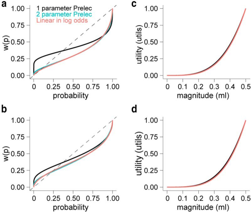
Parametric estimation of probability distortion and utility functions. Trial-by-trial choice data were best explained by a combination of inverted S-shaped probability weighting functions and convex utility functions. a, b, Estimated probability distortion curves using one- or two-parameter weighting functions. The legend in a applies to all panels and describes the specific model used. The estimated probability weighting functions show the traditional overweighting of small probability rewards and underweighting of large probability rewards, for monkeys A and B, respectively. c, d, Estimated power utility functions for monkeys A and B, respectively. The utility functions were nearly overlapping, thus the utility function paired with the two-parameter Prelec model (blue) is not visible because of overlap.

Figure 5.

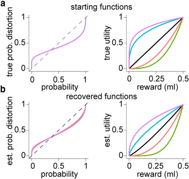
Parametric estimation of simulated probability distortion and utility functions. a, Left, 5 1-parameter probability weighting functions with identical (overlapping) curvature (α = 0.37). Right, 5 utility functions modeled with a power function consisting of terms (in order of decreasing risk aversion) 0.2 (purple), 0.3 (cyan), 1 (black), 2 (red), and 3 (olive). Each utility function was paired with a probability weighting function and together one pair acted as a “starting function” to generate choice data. b, Each pair of starting functions (a) operated on the choice trials presented to monkey A and created gamble or safe choices via a “softmax” algorithm (Eq. 3) followed by a weighted coin flip. We ran the parametric optimization procedure on each of the five simulated datasets. The recovered functions are color coded according to the starting functions shown in a.

We computed the utilities of the choice options using the following:

where w(θ, p) was the weight assigned to probability of getting 0.5 ml given parameters θ and u(0.5 ml) = 1. We chose a power function to model the utility function, as is commonly done (Lattimore et al., 1992; Gonzalez and Wu, 1999; Hsu et al., 2009), where ρ > 1 indicates risk seeking, ρ = 1 indicates risk neutrality, and ρ < 1 indicates risk aversion. For direct comparability with the gamble, the resulting utility functions were normalized such that u(0.5 ml) = 1.

Finally, we investigated three widely used probability distortion models, the one- and two-parameter Prelec functions (Eqs. 6 and 7, respectively, Prelec, 1998) and the linear in log-odds model (Eq. 8, Lattimore et al., 1992; Gonzalez and Wu, 1999):

where α, β, δ, and γ were free parameters. We used an unconstrained Nelder–Mead search algorithm (MATLAB: fminsearch) to minimize the sum of the negative log likelihoods with respect to the utility function, softmax parameter, and probability distortion parameter(s). The log likelihood for each binned gamble-safe pair was given by the following:

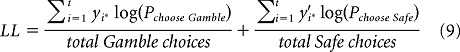where i = trial number, t = total trial number in a bin, and y and y′ were choices for gamble and safe outcomes (1 if chosen, 0 otherwise), respectively. Model comparison was done using Bayesian information criteria (BIC) with the optimized parameters for each model (see Table 1). To verify the validity of this procedure, we repeated this exact procedure on simulated data (see Fig. 5). Simulated choice data were derived from five different decision models consisting of a power utility function and one parameter Prelec probability weighting function. Each model was presented with the same choice trials shown to monkey A and the choices were generated using Equation 3 with a softmax parameter = 1 (which was approximately the value of that parameter estimated from the monkeys' behavior), followed by a weighted coin flip.

Table 1.

Parameter estimates from discrete choice models for monkey A and B

Model	ρ (A, B)	θ1 (A, B)	θ2 (A, B)	λ (A, B)	BIC (A, B)
1 parameter Prelec (θ1 = α)	3.45, 3.62	0.31, 0.47	NA	0.85, 1.44	341.3, 294.6
2 parameter Prelec (θ1 = α, θ2 = β)	3.60, 3.84	0.49, 0.54	1.48, 1.20	0.81, 1.39	347.7, 301.2
Gonzalez and Wu (θ1 = δ, θ2 = γ)	3.61, 3.83	0.41, 0.62	0.63, 0.58	0.80, 1.39	347.7, 301.2

NA, Not applicable.

Results

Basic task and behavioral performance

After extensive conditioning with sector stimuli that indicated gambles and value bars that predicted safe rewards (Fig. 1a–c; see Materials and Methods), monkeys made saccade-guided choices between two cues (Fig. 1d,e). We first investigated whether the animals appropriately used the sector information to select between gambles (Fig. 1d). Both monkeys consistently selected the gamble with higher probability (Fig. 1f, 89% and 82% of the time, monkey A and B, respectively). Their choice behavior on every trial depended on both gamble values (p < 10⁻¹⁰, both animals; logistic regression, Eq. 1), which were determined solely by the gambles' respective probabilities (the outcomes were always 0.5 and 0 ml). Neither animal exhibited a side bias (p = 0.34 and 0.2 in monkey A and B, respectively; logistic regression). Therefore, the monkeys appeared to use the sector stimuli to make meaningful choices and maximize value on a trial-by-trial basis.

Next, we measured choice behavior when the animals selected between a gamble and a safe reward (Fig. 2a). Due to the nature of the cues, these choices were more demanding compared with those between two gambles because the animals could not visually compare the size of shaded regions to determine the more valuable option. Rather, the value of the gamble was determined by the probability of winning (outcomes always 0.5 and 0 ml), whereas the value of the safe option was determined by the offered magnitude (probability = 1). Logistic regression revealed that both values were used in an economically rational way; a higher chance of winning increased the probability of choosing the gamble (Fig. 2b, p = 5.02⁻¹⁰ and 9.44⁻¹² in monkeys A and B, respectively; t test), whereas larger safe magnitude decreased the probability of choosing the gamble (Fig. 2b, p = 7.94⁻¹² and 1.64⁻¹² in monkeys A and B, respectively; t test). As in many previous studies (McCoy and Platt, 2005; O'Neill and Schultz, 2010; Kim et al., 2012; So and Stuphorn, 2012; Lak et al., 2014; Raghuraman and Padoa-Schioppa, 2014), both animals were risk seeking (Fig. 2b, p = 4.62⁻⁶ and 6.22⁻⁸ in monkeys A and B, respectively; t test), but neither animal exhibited a significant side bias (Fig. 2b, p = 0.617 and 0.862 in monkey A and B, respectively; t test).

Although the choices between two gambles indicated that the animals understood the sector stimuli (Fig. 1f), the logistic regression on choices between the gamble and safe reward revealed a small but significant bias toward choosing the gamble over the safe option, even after risk, probability, and reward magnitude had been accounted for (β₀ = 0.5 and 2.2, logistic regression across as trials, p < 10⁻¹⁰ in monkeys A and B; Wald test). There was no significant trend in this bias as a function of chronological session sequence (R² = 0.01 and 0.005, p = 0.08 and 0.8 in monkeys A and B, linear regression between intercept and session number). Likewise, the bias did not appear to reflect a simple cutoff rule according to which the animals chose the gambles when safe reward magnitudes were low (even at low probability). The likelihood of choosing low probability gambles (p < 0.3) did not dramatically increase at low reward magnitudes (Fig. 2c,d). In fact, the only dramatic shift in the likelihood of choosing the gamble occurred when the magnitude of the safe offer was >0.5 ml (Fig. 2c,d, red arrows). When the safe value offered was larger than 0.5 ml, there was no possible benefit to choosing the gamble. That the choice behavior reflected this objective value difference is strong evidence that the monkeys understood the relative value of the options. Therefore, the choice bias did not seem to arise from a gross misunderstanding of the cues. Rather, the bias seemed to reflect misspecification of the logistic model in capturing randomness in the behavior and we corrected for this during parametric analysis by subtracting 60 μl from the safe offer (see Materials and Methods). Because the bias was treated as a constant independent of reward magnitude and probability, it did not contribute to the estimated nonlinearity associated with magnitude (utility) or probability (distortion).

Estimation of probability weighting functions

Choice indifference points between gambles and safe rewards (i.e., CE) are a measure of the subjective value of a gamble. Because the gambles had one nonzero outcome, the CE divided by the nonzero outcome (0.5 ml) provided a measure of probability distortion (Tversky and Kahneman, 1992). A comparison of the resulting data with the identity line indicated that the animals overweighted low probability rewards and underweighted high probability rewards (Fig. 3). However, a significant challenge in identifying probability distortion is the existence of other factors influencing subjective value, namely nonlinear utility functions, which specify the relationship between subjective value and reward magnitude.

Figure 3.

Certainty equivalents indicating probability distortion. a, b, Probability weighting versus nominal probability. Each data point represents a measured certainty equivalent divided by 0.5 ml and normalized so that the smallest and largest measured CEs were equal to 0 and 1, respectively. n = 602 in monkey A and 278 in monkey B. Red lines are identity lines.

To address this challenge, we simultaneously estimated the shape of the underlying probability weighting and utility functions. We used a standard discrete choice model (Eq. 3) to find the set of parameters that best explained the observed choice probability for each gamble-safe alternative option (Materials and Methods, “Behavioral analysis”). We explored classical one- and two-parameter probability weighting functions that are able to capture overweighting, underweighting, or linear treatment of probability (Eqs. 6–8; Lattimore et al., 1992; Prelec, 1998; Gonzalez and Wu, 1999). Likewise, power functions appropriately modeled utility because they easily accommodate diverse risk attitudes (indicating risk neutrality when ρ = 1, risk avoiding when ρ < 1, and risk seeking when ρ > 1; Eq. 5). The estimation procedure placed no constraints or boundaries on the values parameters could take. Table 1 provides the optimized parameters for the three models as well as a model comparison index, the BIC. The one-parameter Prelec model outperformed both two-parameter models (ΔBIC∼6, indicating relatively strong differences, but with the large trial number, BIC places a large penalty on extra parameters; therefore, we plotted all three functions in Fig. 4a,b). The distinctive “inverted S” of the probability weighting functions indicated that both monkeys overweighted lower probability rewards and underweighted high probability rewards (Fig. 4a,b). The crossover point for the best-fitting one-parameter model was near p = 0.37, enforced by the model itself (1/e). Nevertheless, in the other models that do not enforce a specific crossover point, the fitted function crossed the identity line at low probabilities (Fig. 4a,b). The simultaneously estimated utility functions were convex in both monkeys independent of which probability distortion function was used (Fig. 4c,d). Therefore, the utility functions indicated risk seeking and corroborated the positive logistic regression coefficients for risk (Fig. 2b). Together, these results reinforced the commonly observed risk-seeking behavior in monkeys (McCoy and Platt, 2005; O'Neill and Schultz, 2010; Kim et al., 2012; So and Stuphorn, 2012; Lak et al., 2014; Stauffer et al., 2014) and revealed evidence that monkeys exhibit a nonlinear probability weighting function with an inverted S-shaped form.

To ensure that the parameter estimation analysis appropriately attributed weight to the utility and probability weighting functions, we tested the parameter estimation procedure against five simulated datasets for which the true parameter values were known. These simulated choice data were created from five different discrete choice models with identical probability weighting functions (Fig. 5a, left), but broadly spaced utility functions to represent both risk seeking and risk avoiding tendencies (Fig. 5a, right). Each model was presented with the same choice options presented to monkey A (Materials and Methods). In all cases, the parameter estimation technique recovered the true probability distortion function with great fidelity (Fig. 5b, left). Likewise, despite some apparent overestimation of the power term, the technique correctly dissociated the risk averse utility functions from the risk seeking utility functions (Fig. 5b, right). This result indicates that the parameter estimation technique used here adequately assigned weight to the two functions and provided validation for the best-fitting utility and probability distortion functions described above.

Monkeys are risk seeking for small rewards

Probability weighting functions and nonlinear utility can explain some of the same behavioral phenomena such as risk seeking for small probability gambles. However, there are certain situations in which only one or the other is appropriate. To empirically validate the estimated functions and provide evidence for probability distortion that is independent from nonlinear utility (and vice versa), we investigated preferences that cannot be explained by both functions.

The logistic regression analysis (Fig. 2b) and the estimated convex utility functions (Fig. 4c,d) indicated that the monkeys were risk seeking. To empirically validate the presence of convex utility, we measured the CE of a 50:50 gamble between 0.1 and 0.4 ml and compared it with the CE of the 50:50 gamble between 0 and 0.5 ml. The latter gamble is a mean preserving spread of the former (Rothschild and Stiglitz, 1970). Therefore, a risk-seeking individual with a convex utility function will prefer (and should report a higher CE for) the riskier gamble compared with the less risky gamble, reflecting second order stochastic dominance for risk seeking (Fishburn, 1974). Because the probabilities are identical, a risk preference in this situation cannot be attributed to probability distortion. Indeed, monkey B reported a significantly larger CE for the riskier compared with the less risky gamble (Fig. 6a, p = 0.001, t test). We verified this behavior in a third animal (monkey C, Fig. 6a, p = 0.02, t test). This result provides strong evidence in favor of the identified convex utility functions in the tested reward magnitude range (Fig. 4c,d), and agrees with the behavioral results reported previously (McCoy and Platt, 2005; O'Neill and Schultz, 2010; Kim et al., 2012; So and Stuphorn, 2012; Lak et al., 2014; Raghuraman and Padoa-Schioppa, 2014; Stauffer et al., 2014).

Reward probabilities are weighted in a nonlinear fashion

Convex utility functions explain the preference for a riskier gamble that is a mean preserving spread of a less risky gamble with the same reward probability. Here, we investigate whether these utility functions are sufficient to explain preferences for gambles with other reward probability. A hallmark of expected utility (EU) theory is a linear treatment of probability. Therefore, the EU of a binary gamble is calculated according to the following:

where p is the nominal probability and u is the utility function. In contrast, prospect theory and other modern decision theories incorporated probability distortion into the value computation. Therefore, the value (V) of a binary gamble is calculated according to the following:

where w is the weight applied to the probability and ν is a nonlinear value function. To investigate whether the expected utility theory approximated the animals' choice behavior, we estimated utility functions from the CE of 50:50 gambles using a power function (Fig. 6b, light and dark gray correspond to the utility functions from monkeys A and B, respectively). Because the origin and scale of utility functions are arbitrary [u(0.5 ml) = 1 and u(0 ml) = 0], Equation 10 reveals the indicated probability according to EU/1 = p. Likewise, we used the estimated utility functions to calculate the observed probability (p̂) from the utility of the measured CE (u(CE)/1 = p̂). An example is demonstrated for a gamble with reward probability p = 0.25 (Fig. 6b, blue and orange lines). If the subjects were approximating EU-like behavior [i.e., gambles EU ≈ u(CE)], then p should approximate p̂ and there should not be a trend in the difference between the two variables. In fact, the difference between p̂ and p was significantly positive at lower probabilities (95% CI of the mean = 0.04 and 0.07, p = 5.7⁻⁹; t test), suggesting overweighting of low probability outcomes, and significantly negative at higher probabilities (95% CI of the mean = −0.22 and −0.18, p < 10⁻¹⁰; t test), suggesting underweighting of high probability outcomes (Fig. 6c, black dots). The differences were highly correlated with the difference between the estimated one-parameter Prelec probability weighting function and nominal probability (Fig. 6c, green line, ρ = 0.97, p = 3.12⁻¹³; Pearson's correlation). This result demonstrates that convex utility alone is not sufficient to explain the choice data and validates the presence and form of the parametrically estimated probability weighting function shown in Figure 4.

Choices reflect probability rather than recent reinforcement history

The gambles (indicated by the probability cues) remained constant over the course of a PEST sequence (Fig. 7a, left). However, a computerized random number generator determined the actual reward sequence. Therefore, especially on short sequences, the local reinforcement history could provide a relative frequency of rewarded and nonrewarded outcomes that deviated from the indicated probability (Fig. 7a, right). To determine whether reinforcement history explained the apparent probability distortions, we investigated whether the idiosyncratic deviation of reward frequency from indicated probability could explain the deviation of w(p) from identity. The results indicate that local reinforcement history failed to provide extra explanatory power over the indicated probability (Fig. 7b, combined data, R² = 0.001 and p = 0.62 in monkey A, R² = 0.02 and p = 0.12 in monkey B; linear regressions). Indeed, the indicated probability explained a greater portion of the variance compared with the experienced reward frequency in separate linear regressions with w(p) (R² = 0.64 vs 0.55 for indicated probability and experienced reward frequency, respectively, p < 10⁻¹⁰ in both animals, linear regressions). These results suggest that the substantial experience of the monkeys had enabled them to use the indicated reward probability rather than inferring probability from recently experienced outcomes. Moreover, idiosyncratic reinforcement histories did not explain the probability distortion.

Figure 7.

Probability distortions do not reflect recent reinforcement history. a, Local reinforcement history may induce deviation of experienced reward frequencies from indicated probabilities. In the example shown, indicated probability is 0.25 (left), but the gamble was chosen five times and rewarded twice, so the “experienced” frequency is 2/5 = 0.20. S, Safe choice; G, gamble choice; 1, rewarded trial; 0, unrewarded trial. b, Deviation of experienced frequency from indicated probability fails to explain deviation of w(p) from p. Each data point represents one PEST session. The black line represents the best-fit line (R² = 0.005, p = 0.2 combined data both animals; linear regression).

Discussion

This study demonstrated that monkeys distorted reward probability during value-based choices. When making choices between risky and safe rewards, the monkeys appeared to overweight low probability rewards and underweight high probability rewards. The probability distortion was well described by traditional probability weighting functions with an inverted S shape and a crossover point near p = 0.37. To isolate probability distortion, we held the outcome magnitudes (and hence the outcome utilities) constant while varying the probability of winning liquid reward. As in many previous studies, the monkeys were risk seeking for small rewards (McCoy and Platt, 2005; O'Neill and Schultz, 2010; Kim et al., 2012; So and Stuphorn, 2012; Lak et al., 2014; Raghuraman and Padoa-Schioppa, 2014). However, in addition to evidence for convex utility, the analysis of the choice data revealed evidence for classical probability distortion. This result suggests that specific patterns of probability distortion might have an evolutionary origin, perhaps directly founded in neuronal function. Therefore, economic decision making under risk in monkeys could provide the unique possibility of investigating the neurophysiological correlates of probability distortion in a species with sophisticated behavioral capacity.

Probability distortion is a key pillar of behavioral economics. Despite the normative appeal of expected utility theory (von Neumann and Morgenstern, 1944), decision makers often violate fundamental assumptions, such as the independence axiom (Allais, 1953). Therefore, expected utility theory often fails as a descriptive tool (Machina, 1987). Prospect theory, rank-dependent utility theory, and cumulative prospect theory all incorporate probability distortion (Kahneman and Tversky, 1979; Quiggin, 1982; Tversky and Kahneman, 1992). Therefore, our findings in monkeys are highly consistent with basic assumptions of modern decision theories and with studies in humans that revealed probability distortion (Lattimore et al., 1992; Gonzalez and Wu, 1999; Abdellaoui, 2000; Hsu et al., 2009).

Probability distortion and nonlinear utility functions are able to explain some of the same phenomena. However, neither alone was sufficient to explain the data presented here. The CE data (Fig. 3) strongly suggested risk seeking, but it could only be explained by nonlinear utility alone had all the data points stayed on the same side of the identity line. Accordingly, multiplying convex utility functions with nominal probabilities (according to expected utility theory) underestimated the CE of low probability rewards and overestimated the CE of high probability rewards (thus indicating overweighting and underweighting of low and high probability rewards, respectively, Fig. 6b,c). Therefore, convex utility alone was not adequate to explain the subjective values measured for gambles with different probability. Conversely, monkeys preferred the riskier of two gambles with the same mean and probability but different outcome magnitudes (Fig. 6a). This preference between mean preserving options cannot be explained by probability distortion (because the reward probabilities are identical), but is entirely consistent with convex utility functions. Together, these results from the full range of the extensively tested behavioral situations indicate the presence of nonlinearity in both utility and probability weighting functions.

Probability distortion is commonly invoked to explain the “fourfold pattern of risk attitudes” that spans the gain and loss domain around a reference point (Kahneman and Tversky, 1979). However, in this study there is the lack of a well defined reference point, so it is unclear whether the “unlucky” outcomes can be described as losses. Some economic theories incorporate the rational expectation (Koszegi and Rabin, 2006) or the CE of the gamble (Gul, 1991) as a natural reference point; however, the traditional reference point is the status quo (Kahneman and Tversky, 1979). In the former two models, the unlucky gamble outcome used here (0 ml) would be considered a loss, whereas in the latter model it would not. It is therefore not clear whether the unlucky gamble outcome used in this study can be considered a genuine loss. Nevertheless, analysis of probability distortion has commonly been restricted to the gain domain (Gonzalez and Wu, 1999) or characterized in the absence of a reference point, as in rank dependent utility (Quiggin, 1982). Therefore, the current methods and results are entirely consistent with established behavioral economic theory.

The means by which probability is known leads to differently formed probability weighting functions. In previous research on instructed probability, individuals overweighted small probability outcomes and underweighted larger ones (the classical inverted S form shown here). Conversely, when probabilities were learned from experience, the opposite pattern was often observed; individuals exhibited underweighting of low chance events and overweighting of high chance events (Hertwig et al., 2004; Hertwig and Erev, 2009). In our behavioral task, we deliberately used an explicit representation of probability (sector stimuli) to mimic instruction rather than experience. Initially, the animals had to learn the meaning of the sectors, which added an initial element of experience to this study. However, the impact of this experience element should decrease over thousands of learning trials. Consistent with this argument, analysis of the choice data revealed that the indicated (instructed) probability was a better explanatory variable than the local reward history (Fig. 7). Moreover, the experience component here remains qualitatively different from real world decision making. In the real world, rare events are normally undersampled. In contrast, our animals commonly experienced 300–500 trials per day, so even the low probability events were generously sampled. Accordingly, the probability distortion conformed to the inverted S shape normally associated with instructed probability.

Both animals accurately selected between two risk cues, but the logistic regression revealed a bias that arose when they made choices between safe and risky options. This indicated that after magnitude, risk, and probability had been considered, both monkeys were still more likely to choose the gamble over the safe option. Importantly, this bias appeared not to arise from a gross misunderstanding of the two cue types, or their relative values. First, when the animals selected between two gambles, they chose the higher value option the majority of the time (Fig. 1f). Second, when the magnitude of the safe offer was greater than the winning outcome of the gamble, both monkeys correctly chose the safe offer (Fig. 2c,d). Finally, the bias did not decrease as a function of sequential session, indicating that there was no ongoing learning; that is, the animals were not “getting better” at the task over time. Therefore, although both animals selected the risky option more often than the models accounted for, they appeared to understand the relative value of the choice options and behaved in an economically reasonable way.

The observed similarity in probability weighting functions between human and nonhuman primates suggests that similar neuronal mechanisms might be engaged. Previous functional imaging studies have found evidence of probability distortion in the brain in both choice and nonchoice tasks (Tobler et al., 2008; Hsu et al., 2009). However, no study has examined probability distortion at the single-cell level. Reward probability modulates the activity of neurons in the midbrain dopamine system (Fiorillo et al., 2003), the striatum (Samejima et al., 2005; Lau and Glimcher, 2008), parietal cortex (Platt and Glimcher, 1999; Yang and Shadlen, 2007), the orbitofrontal cortex (Kennerley et al., 2011; Raghuraman and Padoa-Schioppa, 2014), and other frontal cortex structures (Kennerley et al., 2011; So and Stuphorn, 2012). A question to ask is whether reward probability is distorted during simple reward prediction tasks or if a distorted reward probability representation only arises during choice. Such a study could illuminate whether probability distortion arises out of faulty beliefs about probability itself or if the behavioral manifestation of probability distortion represents a limit on neuronal processing capacity that is exceeded by the demands of value-based decisions. The explicit probability cues used here appear to offer a flexible and dynamic means to neurophysiologically investigate this important behavioral phenomenon. Indeed, the sector cues were constructed with this application in mind. The horizontal and vertical hatched areas indicating probability of reward and no reward, respectively, ensure that the luminance and physical salience of every indicated probability is identical. This design enables well controlled investigation of neuronal responses.

In summary, the current choice data suggest that monkeys distort indicated reward probabilities when making economic choices. Traditional models of probability distortion provide a good model for this behavior in monkeys. The similarity between the inverted S-shaped probability weighting function in monkeys and humans suggests that this phenomenon may have an evolutionary origin, perhaps preserved in common neuronal processes. This study thus lays the foundation for an in depth neurophysiological investigation of how probability is combined with utility to guide choice behavior.

References

- Abdellaoui M. Parameter-free elicitation of utility and probability weighting functions. Management Science. 2000;46:1497–1512. doi: 10.1287/mnsc.46.11.1497.12080. [DOI] [Google Scholar]
- Allais M. Le Comportement de l'Homme Rationnel devant le Risque: Critique des Postulats et Axiomes de l'Ecole Americaine. Econometrica. 1953;21:503–546. [Google Scholar]
- Fiorillo CD, Tobler PN, Schultz W. Discrete coding of reward probability and uncertainty by dopamine neurons. Science. 2003;299:1898–1902. doi: 10.1126/science.1077349. [DOI] [PubMed] [Google Scholar]
- Fishburn P. Convex stochastic dominance with continuous distribution functions. Journal of Economic Theory. 1974;7:143–158. doi: 10.1016/0022-0531(74)90103-3. [DOI] [Google Scholar]
- Frydman C, Camerer C, Bossaerts P, Rangel A. MAOA-L carriers are better at making optimal financial decisions under risk. Proc R Soc B. 2011;278:2053–2059. doi: 10.1098/rspb.2010.2304. [DOI] [PMC free article] [PubMed] [Google Scholar]
- Gonzalez R, Wu G. On the shape of the probability weighting function. Cognitive Psychology. 1999;166:129–166. doi: 10.1006/cogp.1998.0710. [DOI] [PubMed] [Google Scholar]
- Gul F. A theory of disappointment aversion. Econometrica. 1991;59:667–686. doi: 10.2307/2938223. [DOI] [Google Scholar]
- Hertwig R, Erev I. The description-experience gap in risky choice. Trends Cogn Sci. 2009;13:517–523. doi: 10.1016/j.tics.2009.09.004. [DOI] [PubMed] [Google Scholar]
- Hertwig R, Barron G, Weber EU, Erev I. Decisions from experience and the effect of rare events in risky choice. Psychol Sci. 2004;15:534–539. doi: 10.1111/j.0956-7976.2004.00715.x. [DOI] [PubMed] [Google Scholar]
- Hsu M, Krajbich I, Zhao C, Camerer CF. Neural response to reward anticipation under risk is nonlinear in probabilities. J Neurosci. 2009;29:2231–2237. doi: 10.1523/JNEUROSCI.5296-08.2009. [DOI] [PMC free article] [PubMed] [Google Scholar]
- Kahneman D, Tversky A. Prospect theory: an analysis of decision under risk. Econometrica. 1979;47:263–291. doi: 10.2307/1914185. [DOI] [Google Scholar]
- Kennerley SW, Behrens TE, Wallis JD. Double dissociation of value computations in orbitofrontal and anterior cingulate neurons. Nat Neurosci. 2011;14:1581–1589. doi: 10.1038/nn.2961. [DOI] [PMC free article] [PubMed] [Google Scholar]
- Kim S, Bobeica I, Gamo NJ, Arnsten AFT, Lee D. Effects of α-2A adrenergic receptor agonist on time and risk preference in primates. Psychopharmacology (Berl) 2012;219:363–375. doi: 10.1007/s00213-011-2520-0. [DOI] [PMC free article] [PubMed] [Google Scholar]
- Koszegi B, Rabin M. A model of reference dependent preferences. Q J Econ. 2006;121:1133–1165. [Google Scholar]
- Lak A, Stauffer WR, Schultz W. Dopamine prediction error responses integrate subjective value from different reward dimensions. Proc Natl Acad Sci U S A. 2014;111:2343–2348. doi: 10.1073/pnas.1321596111. [DOI] [PMC free article] [PubMed] [Google Scholar]
- Lattimore PK, Baker JR, Witte AD. The influence of probability on risky choice: a parametric examination. Journal of Economic Behavior and Organization. 1992;17:377–400. doi: 10.1016/S0167-2681(95)90015-2. [DOI] [Google Scholar]
- Lau B, Glimcher PW. Value representations in the primate striatum during matching behavior. Neuron. 2008;58:451–463. doi: 10.1016/j.neuron.2008.02.021. [DOI] [PMC free article] [PubMed] [Google Scholar]
- Luce DR. Utility of gains and losses: measurement-theoretic and experimental approached. Mahwah, NJ: Lawerence Erlbaum Associates; 2000. [Google Scholar]
- Machina M. Choice under uncertainty: problems solved and unsolved. Economic Perspectives. 1987;1:121–154. doi: 10.1257/jep.1.1.121. [DOI] [Google Scholar]
- McCoy AN, Platt ML. Risk-sensitive neurons in macaque posterior cingulate cortex. Nat Neurosci. 2005;8:1220–1227. doi: 10.1038/nn1523. [DOI] [PubMed] [Google Scholar]
- O'Neill M, Schultz W. Coding of reward risk by orbitofrontal neurons is mostly distinct from coding of reward value. Neuron. 2010;68:789–800. doi: 10.1016/j.neuron.2010.09.031. [DOI] [PubMed] [Google Scholar]
- Platt ML, Glimcher PW. Neural correlates of decision variables in parietal cortex. Nature. 1999;400:233–238. doi: 10.1038/22268. [DOI] [PubMed] [Google Scholar]
- Prelec D. The probability weighting function. Econometrica. 1998;66:497–527. doi: 10.2307/2998573. [DOI] [Google Scholar]
- Quiggin J. A theory of anticipated utility. Journal of Economic Behavior and Organization. 1982;3:323–343. doi: 10.1016/0167-2681(82)90008-7. [DOI] [Google Scholar]
- Raghuraman AP, Padoa-Schioppa C. Integration of multiple determinants in the neuronal computation of economic values. J Neurosci. 2014;34:11583–11603. doi: 10.1523/JNEUROSCI.1235-14.2014. [DOI] [PMC free article] [PubMed] [Google Scholar]
- RCoreTeam. R: A language and environment for statistical computing. R Foundation for Statistical Computingtle. 2014 [Google Scholar]
- Rothschild M, Stiglitz J. Increasing risk: I. A definition. Journal of Economic Theory. 1970;2:225–243. doi: 10.1016/0022-0531(70)90038-4. [DOI] [Google Scholar]
- Samejima K, Ueda Y, Doya K, Kimura M. Representation of action-specific reward values in the striatum. Science. 2005;310:1337–1340. doi: 10.1126/science.1115270. [DOI] [PubMed] [Google Scholar]
- So N, Stuphorn V. Supplementary eye field encodes reward prediction error. J Neurosci. 2012;32:2950–2963. doi: 10.1523/JNEUROSCI.4419-11.2012. [DOI] [PMC free article] [PubMed] [Google Scholar]
- Stauffer WR, Lak A, Schultz W. Dopamine reward prediction error responses reflect marginal utility. Curr Biol. 2014;24:2491–2500. doi: 10.1016/j.cub.2014.08.064. [DOI] [PMC free article] [PubMed] [Google Scholar]
- Tobler PN, Christopoulos GI, O'Doherty JP, Dolan RJ, Schultz W. Neuronal distortions of reward probability without choice. J Neurosci. 2008;28:11703–11711. doi: 10.1523/JNEUROSCI.2870-08.2008. [DOI] [PMC free article] [PubMed] [Google Scholar]
- Tversky A, Kahneman D. Advances in prospect theory: cumulative representation of uncertainty. Journal of Risk and Uncertainty. 1992;5:297–323. doi: 10.1007/BF00122574. [DOI] [Google Scholar]
- Von Neumann J, Morgenstern O. Theory of games and economic behavior. Princeton: Princeton University; 1944. [Google Scholar]
- Wickham H. ggplot2: elegant graphics for data analysis. 2009 [Google Scholar]
- Yamada H, Tymula A, Louie K, Glimcher PW. Thirst-dependent risk preferences in monkeys identify a primitive form of wealth. Proc Natl Acad Sci U S A. 2013;110:15788–15793. doi: 10.1073/pnas.1308718110. [DOI] [PMC free article] [PubMed] [Google Scholar]
- Yang T, Shadlen MN. Probabilistic reasoning by neurons. Nature. 2007;447:1075–1080. doi: 10.1038/nature05852. [DOI] [PubMed] [Google Scholar]