Novel microscale approaches for easy, rapid determination of protein stability in academic and commercial settings

Abstract

Chemical denaturant titrations can be used to accurately determine protein stability. However, data acquisition is typically labour intensive, has low throughput and is difficult to automate. These factors, combined with high protein consumption, have limited the adoption of chemical denaturant titrations in commercial settings. Thermal denaturation assays can be automated, sometimes with very high throughput. However, thermal denaturation assays are incompatible with proteins that aggregate at high temperatures and large extrapolation of stability parameters to physiological temperatures can introduce significant uncertainties. We used capillary-based instruments to measure chemical denaturant titrations by intrinsic fluorescence and microscale thermophoresis. This allowed higher throughput, consumed several hundred-fold less protein than conventional, cuvette-based methods yet maintained the high quality of the conventional approaches. We also established efficient strategies for automated, direct determination of protein stability at a range of temperatures via chemical denaturation, which has utility for characterising stability for proteins that are difficult to purify in high yield. This approach may also have merit for proteins that irreversibly denature or aggregate in classical thermal denaturation assays. We also developed procedures for affinity ranking of protein–ligand interactions from ligand-induced changes in chemical denaturation data, and proved the principle for this by correctly ranking the affinity of previously unreported peptide–PDZ domain interactions. The increased throughput, automation and low protein consumption of protein stability determinations afforded by using capillary-based methods to measure denaturant titrations, can help to revolutionise protein research. We believe that the strategies reported are likely to find wide applications in academia, biotherapeutic formulation and drug discovery programmes.

Graphical abstract

Highlights

• •Chemical denaturant titrations are slow, lengthy and consume lots of protein sample.
• •We developed very fast methods for measuring chemical denaturant titrations.
• •Automated titrations can be measured in minutes using only μl sample volumes.
• •Ligand interactions rapidly screened and ranked via changes in protein stability
• •These advances make chemical denaturation more suitable for commercial research.

1. Introduction

1.1. Protein denaturation: principles and applications

Equilibrium denaturation experiments are widely used to quantify how changes in pH, temperature, or the presence of different additives affect protein stability [1–7]. These experiments yield insights into the forces driving protein folding and misfolding dynamics, and their linkage with function and disease [8–12]. Moreover, protein stability is of direct relevance to optimising the formulation and storage of clinical antibodies and biotherapeutic proteins (see Section 3.3) [1–3].

When quantifying the relative stability of the native protein (N), the denatured state (D) is typically used as a reference state [5]. The relative population of different states under specific conditions defines the equilibrium constant (K_eq). The difference in free energy between D and N (i.e. G_D − G_N, Fig. S1a), can be calculated from ΔG_D–N = −RT·lnK_eq (where R is the gas constant and T the temperature) [9,13,14]. Equilibrium denaturation measurements are exceptionally powerful when combined with systematic protein mutagenesis (the ‘protein engineering method’) [5,8,15,16]. This allows changes in ΔG_D–N for a mutant protein to be compared to the wild-type value (ΔΔG_D–N, Fig. S1a) and can yield atomic resolution insights into the origins of protein folding and stability, but typically requires the stability of 40–100 protein variants to be determined [17,18].

Protein denaturation can be mediated using mechanical, thermal or chemical methods. Mechanical methods involve stretching a protein until it unfolds (e.g. atomic force microscopy) [15]. Whilst mechanical methods provide unique insights, they are technically challenging and require highly specialised, expensive instrumentation (which has limited their widespread adoption). Thermal denaturation methods involve gradually heating samples whilst recording changes in experimental parameters that discriminate the properties (and populations) of native and denatured conformers. Differential scanning calorimetry (DSC), circular dichroism (CD) and nuclear magnetic resonance (NMR) spectroscopy are popular, gold standard analytical techniques for probing thermal denaturation (although CD and NMR are not thermal denaturation methods per se and are more routinely used for making measurements at a single temperature) [6,7,19]. The need for gradual heating means that thermal denaturation experiments cantake several hours, even when employing robotic platforms. Differential scanning fluorimetry (DSF) and isothermal denaturation (ITD) are thermal denaturation methods commonly used to screen protein–ligand interactions from changes in melting temperature (T_m, as in DSF) or the kinetics of denaturation (as in ITD) [1,2,20]. Very high throughput can be achieved in DSC and ITD experiments by multiplexing the measurements (e.g. making many measurements in parallel using 384-well microtitre plates) [1,2,20]. High percentages are amenable to thermal denaturation assays. However, this technique is not universally applicable, as some proteins aggregate irreversibly at elevated temperatures, which precludes rigorous thermodynamic analyses (since a true equilibrium cannot be established under such circumstances). Whilst protein stability can often be accurately determined at the melting temperature (T_m), significant extrapolations to lower, physiological temperatures (e.g. for a thermostable proteins with a high T_m value) can introduce considerable errors into ΔG_D–N [3,6,13,21].

More proteins denature reversibly in chemical denaturant titrations than in thermal denaturation experiments [3,21]. For example, Freire et al. have measured the anti-EGFR monoclonal antibody using DSC and showed that the data from an initial thermal denaturation were not recapitulated upon subsequent re-scanning [3]. By contrast, chemical denaturation of anti-EGFR antibody with urea was highly reproducible before or after denaturation with 9 M urea [3]. This high incidence of reversibility, combined with chaotropes being cheap and compatible with many buffers, makes chemical denaturation the academic's preferred method for measuring protein stability [22]. Chaotropes, such as urea or guanidinium chloride (GdmCl), have been empirically shown to vary ΔG_D–N in a quasi-linear manner by selectively stabilising denatured conformers Eq. (1) [7,13,14,23]:

$$\mathrm{\Delta }{G}_{\mathrm{D}-\mathrm{N}}=\mathrm{\Delta }{G^0}_{\mathrm{D}-\mathrm{N}}-m_{\mathrm{D}-\mathrm{N}}\cdot \left[\mathrm{Denaturant}\right]$$ (1)

where ΔG_D−N⁰ is protein stability in the absence of a denaturant and m_D–N is derived from the gradient of the unfolding transition (which correlates with changes in accessible surface area accompanying denaturation (Fig. S1b)) [13,14,23]. Thus, ΔG_D–N may be determined by varying the denaturant concentration and observing the relative changes in the populations of N and D (Fig. 1).

Fig. 1.

Chemical denaturation of a protein at equilibrium. Simulated 2-state denaturation induced by increasing the chemical denaturant concentration. The spectroscopic signal used to probe denaturation is typically sigmoidal (black triangles) and consistent with cooperative unfolding [13,14,16]. In order to determine the fractional occupancy of native and denatured states, it is necessary to fit the slopes of pre- (native) and post-transition (denatured) baselines to linear functions (dashed lines). The ΔG_D−N⁰ value can be easily determined by linear extrapolation once the transition midpoint ([Denaturant]_50%) and m_D–N values are known (see Eq. (1), see Section 1.1). m_D–N correlates with the slope of the transition (grey line) and increases with protein size (Fig. S1b) [13,23].

In equilibrium denaturant titrations, the target protein (at a fixed concentration) is titrated into increasing chaotrope concentrations. Solutions are extensively equilibrated to ensure that the system reaches equilibrium, including cis–trans isomerisation of proline residues [8,24]. Each point of this titration is measured using a technique that distinguishes N from D (see Table 1), yielding sigmoidal curves for 2-state reactions (where only N and D are significantly populated, Fig. 1) [16]. However, researchers are typically interested in protein stability in the absence of denaturant (ΔG_D−N⁰), which can be simply calculated from ΔG_D−N⁰ = m_D − N ⋅ [Denaturant]_50 % (since ΔG_D–N equals zero at the transition midpoint, [Denaturant]_50%, see Eq. (1)) [13,14,23,24]. Whilst [Denaturant]_50% is generally the most robustly determined parameter, it is more challenging to accurately determine m_D–N (especially for large proteins where transition regions are narrow, Fig. S1b) [25]. Thus, high data densities are frequently used to improve curve fitting precision (Fig. 1). Differences in stability between proteins, or mutants of the same protein, are generally assumed to be significant if ΔΔG_D–N is ≥ 0.5 kcal/mol [5,10,15,18]. However, whilst this is a widely used threshold within the protein folding community, other values may be applicable depending on the m_D–N values under study (since large proteins have larger m_D–N values and more precise [Denaturant]_50% values than smaller proteins, which have smaller m_D–N values and less precise [Denaturant]_50% values (Fig. S1)).

Table 1.

Common techniques used to measure chemical denaturant titrations.

	NMR	Far-UV CD	Cuvette-based FES	NT.LabelFree FES	NT.LabelFree thermophoresis
Probes	13C, 15N or 1H nuclei	Secondary structure	Tertiary structure	Tertiary structure	Solvation shell
Typical [protein]	50 μM–5 mM	5–100 μM	0.5–100 μM	0.1–100 μM	2–20 μM
Sample vol. per titrationa	5–10 ml	8–15 ml	16–50 ml	0.2–0.5 ml	0.2–0.5 ml
Total sample per titration	15–30 mg	1–2 mg	0.5–1 mg	5–10 μga	5–10 μgb
Time per titration	1–3 days	2–4 h	2–3 h	25 min	45–60 minc
Sample limitations	Proteins usually small (typically < 30 kDa)	Avoid proteins with weak signal changes	Non-fluorescent proteins invisible	Non-fluorescent proteins invisible	Works best for slow folding proteins
Automation	Automated sample changers available	User input needed for each sample	User input needed for each sample	Semi-automated. No washing steps	Semi-automated. No washing steps
Buffer limitations	Avoid protonated buffers in 1H NMR (e.g. Tris)	Avoid chiral buffers (e.g. MES, DTT)	All buffers suitable	All buffers suitable	All buffers suitable
Additional comments	Expensive isotope-enriched protein samples are needed. Yields atomic resolution insights	Chaotropes or buffers can limit the dynamic range of CD instruments	Extrinsic dyes can be used as reporters (but may perturb stability).	Probes chemical and thermal denaturation. ΔGD–Nvs. T measured directly	Excellent for ligand binding. Quality control: aggregates visible in raw data

^aAssuming titrations employ different samples for each denaturant concentration, which is by far the most widely used strategy for chemical denaturant titrations.

^bAssuming similar protein concentrations to those employed here (~ 2 μM).

^cFor titrations containing 48 data points (i.e. 3 × 16 distinct denaturant concentrations measured using Monolith NT.LabelFree instrument, see Materials and methods).

The most commonly used techniques for chemical denaturant titrations are intrinsic fluorescence emission spectroscopy (FES), circular dichroism (CD) and NMR spectroscopy (Table 1) [19,26]. Chemical denaturant titrations involve 30–50 samples (typically with volumes of 0.2–1.0 ml) being sequentially loaded by hand into cuvettes and thereafter thermostated for a defined duration before making measurements. Thus, these experiments are repetitive and take skilled operators 2–4 h to complete (Table 1). Whilst CD and FES spectrometers can be daisy-chained with auto-titrators, these devices consume more protein than manual titrations and offer no real speed advantage (since proteins must be fully equilibrated between denaturant injections for a true equilibrium to be established).

Plate readers can accelerate the measurement of chemical denaturant titrations and reduce sample consumption to as low as 5–10 μl per data point (especially when a covalently attached fluorophore with a high quantum yield is used to probe protein denaturation). However, our experience is that even quartz plates have variations in plate geometry and sample menisci that cause unacceptable data scatter in denaturant titrations (NF, CMJ, unpublished data). Furthermore, injudicious use of extrinsic fluorescent probes can affect the stability of protein targets or introduce unwanted experimental complications [27–29]. For example, extrinsic labelling of proteins can, in some cases, be problematic, requiring protein engineering to provide a suitable residue to which fluorescent dyes can be covalently coupled and it can be time-consuming to separate labelled and unlabelled proteins. Despite the clear advantages of chemical denaturant titrations, their tediousness and relatively high protein consumption has historically prevented their widespread adoption in commercial settings.

1.2. Overview of microscale thermophoresis and associated instrumentation

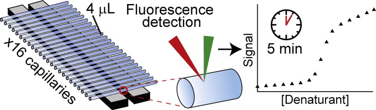
Here we report strategies that greatly simplify and accelerate equilibrium denaturant titrations, without compromising data quality. We used capillary-based instrumentation to measure denaturant titrations in two ways (Fig. 2): (i) using sensitive label-free instruments as low-volume fluorimeters to detect intrinsic fluorescence emission changes accompanying denaturation; and (ii) probing chemical denaturation using microscale thermophoresis (MST) [30–32]. Microscale thermophoresis (MST) describes the directed movement of molecules along μm-sized temperature gradients [30–32]. The movement of protein molecules within a small focal volume on this temperature gradient may be followed by either the extrinsic fluorescence of a covalently attached fluorophore or, in the case of the label-free instruments used here, intrinsic fluorescence emitted by tryptophan residues (Fig. 2) [30–32].

Fig. 2.

Layout of the microscale thermophoresis instrument and measurement principles. (A) MST is measured in disposable capillaries that hold sample volumes of ~ 4 μl. The sample temperature is regulated by thermal elements which directly contact these capillaries. A focused IR laser induces a local temperature gradient in the sample (typically in the order of 2–6 K), triggering thermophoretic movement of molecules [30,31]. Fluorescent molecules in the capillary are excited and detected through the same objective lens. (B) During an MST experiment, the fluorescence of molecules in solution (yellow dots) is detected over time. For simple FES experiments, detection of the initial fluorescence for 1–5 s is sufficient. During a typical MST experiment, the infrared laser is activated after 5 s, resulting in thermophoresis towards lower temperatures which can be quantified by measuring the fluorescence decay (in case of positive thermophoresis, as shown here), or fluorescence increases (negative thermophoresis). After a defined time, the infrared laser is switched off, resulting in re-equilibration of the solution by diffusion.

MST reports on factors affecting solvation entropy of the fluorescent molecule (including changes in size, conformation and charge) [30–32]. Consequently, MST is typically used to quantify molecular interactions, since binding of a ligand alters at least one of these physical parameters. As a protein's solvation shell is significantly affected by denaturation, MST can also be used to detect protein unfolding [10]. However, given that protein folding is usually accompanied by changes in the emission of tryptophan fluorescence, label-free MST instruments allow denaturant titrations to also be measured using intrinsic fluorescence emission.

Importantly, capillary-based denaturant titrations can be measured 5–30 times faster, whilst consuming 40–200 times less protein than existing cuvette-based approaches (including CD and fluorescence spectrometers, Table 1). Further, measurements using capillary-based instruments are semi-automated, allowing a single operator to perform 25–50 titrations per day. They can also automatically re-measure chemical denaturant titrations over a range of temperatures, allowing the temperature-dependence of thermodynamic parameters to be determined hands-free and without exposing proteins to the high temperatures that can cause aggregation in some proteins. We also show that our approach can also be used to screen for ligand-induced changes in protein stability, which has value for therapeutic targets or potentially proteins that behave badly in thermal denaturation screening assays (although this will require further work to verify) [3,30,31]. We believe that these advances in throughput, material consumption and ease-of-use can help to revolutionise protein research in academic and commercial settings.

2. Materials and methods

2.1. Reagents

Ultrapure urea and guanidinium chloride were purchased from MP Biomedicals (CA, USA). All other reagents were purchased from Sigma Chemical Co. (MO, USA) or ThermoFisher (MA, USA). The C-amidated, N-acetylated AWPAK peptide was synthesised by ChinaPeptides (Shanghai, China). SOD1 H43Y noloops and Escherichia coli cytochrome b₅₆₂ F65W proteins were donated by Mikael Oliveberg (University of Stockholm) and Paul Barker (Cambridge University), respectively. α-Spectrin expression vectors were gifts from Jane Clarke (Cambridge University). LQRRRETQV and LQRRRETQ-Abu peptides and the PDZ1 expression vector were gifts from Per Jemth (Uppsala University). Barley chymotrypsin inhibitor-2 (CI2), murine FBP28 WW domain, hepatitis B core protein, the PDZ1 of the post-synaptic density protein 95 (PSD-95) with the F95W mutation (PDZ1 F95W) and α-spectrin constructs were expressed and purified as reported [10,16,33,34]. Protein concentrations were determined spectrophotometrically from calculated molar extinction coefficients.

2.2. Denaturant titrations

Buffers for denaturant solutions (Table S2) were prepared gravimetrically in volumetric flasks to avoid inaccuracies caused by denaturant effects on pH electrodes. Buffered denaturant stocks were prepared similarly and contained urea or GdmCl at concentrations close to their solubility limits (~ 10 M and 8 M, respectively). Denaturant concentrations were accurately determined using refractometry. Concentrated proteins (in the same buffers) were then diluted into buffered denaturant-free or denaturant stocks (see Table S2). These solutions were thoroughly mixed (by pipetting) and equilibrated for at least 1 h before measurements (to allow complete equilibration). This procedure yielded titrations with up to 48 different denaturant concentrations. To characterise the effect of peptide binding on the stability of PDZ1 F95W, a constant volume of water or peptide was added to protein-containing stocks before pipetting the titration.

2.3. Spectroscopic measurements

Far-UV CD spectroscopy was performed using a Jasco J810 spectropolarimeter (Jasco, MD) and 1 mm pathlength cuvettes (Hellma, Germany). The ellipticity of a 70 μM SOD1 sample at 215 nm was measured 60 times (over 1 min) to yield a mean ellipticity value for each denaturant concentration. The ellipticity at 222 nm of a 10 μM sample of the P60A mutant of the R16 α-spectrin domain was recorded from 293 to 368 K to probe thermal denaturation (using a scan rate of 0.1 K/min). Fluorescence emission measurements were made using an Aminco-Bowman SLM2 spectrometer (ThermoFisher, MA) and a 4 × 10 mm pathlength cuvette (Hellma, Germany, excitation and emission pathlengths, respectively). Intrinsic fluorescence was excited at 280 nm (2.5 nm slit-width) and emission recorded twice between 300 and 400 nm (2.5 nm slit-width, 60 nm/min scan rate). The averaged intensity at a given wavelength was plotted vs denaturant concentration to yield denaturant titrations.

2.4. Intrinsic fluorescence emission studies using MST instrumentation

Measurements were performed using a Monolith NT.LabelFree instrument (NanoTemper Inc., Germany). ~ 4 μl of each sample was aspirated into standard-treated glass capillaries by capillarity (NanoTemper Inc., Germany). Capillaries were loaded into a 16-capillary sample holder and thermostated inside the instrument (at 298 K, unless stated otherwise) for ~ 5 min before measurements. The excitation at 280 nm (20 nm bandwidth) was optimised by varying the LED power (from 3 to 25%, Table S2) to yield emission intensities from 330 to 380 nm of 6000–25,000 A.U. This intensity was always > 500 A.U. above background signal intensity. Intrinsic fluorescence was measured for 1–5 s in the absence of a heat gradient. Capillaries were loaded into the instrument as three sets of 16 point titrations (to yield a final titration with up to 48 denaturant concentrations). To avoid systematic errors, these sets were taken from intercalated points in each complete titration (i.e. the first data set contained data points 1, 4, 7…etc., whereas the second set contained data points 2, 5, 8..... etc.). This procedure yielded excellent titrations for most of the proteins that we examined.

2.5. Thermophoresis measurements

Thermophoresis measurements for SOD1 or the AWPAK peptide were performed as described above (also see Table S2), but employing thermal gradients of 2–6 K. Gradients were induced by an infra-red laser using laser powers of 30% (SOD1) or 20–80% (AWPAK peptide) [31]. Fluorescence emission was recorded for 5 s before and after the laser was switched on (Fig. 4B), with data collection throughout. The temperature gradient was maintained for ~ 30 s. Data were normalised to an arbitrary initial fluorescence value of 1. Thermophoresis is the ratio of normalised signals between two time-points after switching the laser on (typically ~ 1 and ~ 29 s, with data averaged within a 0.5–1 s window at each time-point). Normalised values were multiplied by 1000 by the instrumental software.

Fig. 4.

Variance in replicate measurements of denaturant titrations. The variance in triplicate measurements of chemical denaturant titrations was determined (using an NT.LabelFree instrument) for the F65W mutant of E. coli cytochrome b₅₆₂. The data shown is the average of three independent measurements with the standard deviation of measurements represented as error bars. The absolute variation between measurements was ~ 1–2%.

MST was used to measure the interaction between PDZ1 F95W and peptides. A 1 mM peptide stock was serially diluted (1:1) with 50 mM Tris buffer pH 7.5, 150 mM NaCl, 10 mM MgCl₂, 0.05% (v/v) Tween to yield a titration containing sixteen peptide concentrations. PDZ1 F95W was then added at a final concentration of 5 μM and thermophoresis measured in MST-grade standard-treated capillaries at 298 or 310 K. Thermophoresis was induced using laser powers of 20% (at 310 K) or 40% (at 298 K). Thermophoresis was defined as the ratio of signals within a 1 s time window ~ 1 s and ~ 20 s after the laser was switched on. The titrations were fit to Eq. (2) using the manufacturer's software.

$$\mathrm{Signal}=U+\frac{B-U}{2\cdot \left[P\right]}\cdot \left(\left[P\right]+\left[L\right]+K_{\mathrm{d}}-\sqrt{{\left(\left[P\right]+\left[L\right]+K_{\mathrm{d}}\right)}^2-4\cdot \left[P\right]\cdot \left[L\right]}\right)$$ (2)

where [P] and [L] are concentrations of total protein and ligand and U and B represent signals of the unbound and bound states, respectively.

2.6. Thermal scans in MST instruments

10 μl samples of the P60A mutant of R16 α-spectrin, containing a range of urea concentrations, were loaded into standard-treated, zero background MST-grade capillaries to increase signal to noise ratios. Measurements were made using a Monolith NT.LabelFree instrument (NanoTemper Inc., Germany), as described above. Capillaries were sealed with wax to reduce sample evaporation. 16 capillaries were loaded into the instrument and intrinsic fluorescence measured in the absence of a temperature gradient (using a 3% LED power at 295.7 K). After each titration, the temperature was automatically ramped in 2.5 K increments (with 15 min equilibrations between titrations to ensure equilibration).

2.7. Curve fitting

Denaturant titrations were analysed using SigmaPlot (Systat Software, CA). Obvious outlying data points were removed and data fitted to Eq. (2), which describes 2-state protein denaturation [16]. As the slopes of pre- and post-transition baselines can vary linearly with chaotrope concentration (Fig. 1), these were variables in curve fitting of denaturation titrations:

$$F=F_{\mathrm{N}}-\left(F_{\mathrm{N}}-F_{\mathrm{D}}\right).\frac{\exp \left(m\cdot \left(\left[\mathrm{Denaturant}\right]-{\left[\mathrm{Denaturant}\right]}_{50\%}\right)\right)/RT}{1+\exp \left(m\cdot \left(\left[\mathrm{Denaturant}\right]-{\left[\mathrm{Denaturant}\right]}_{50\%}\right)\right)/RT}$$ (3)

where F_N and F_D represent the slopes of the pre- and post-transition baselines, respectively, R is the gas constant, T is the temperature (in K) and [Denaturant]_50% is the denaturant concentration at the transition midpoint.

In experiments probing the thermal dependence of the chemical denaturation of R16 P60A, m was a shared parameter in curve fitting but [Denaturant]_50% was allowed to freely vary at each temperature. This allowed ΔG_D−N⁰ to be determined at a range of temperatures. The resultant trend fitted satisfactorily to a polynomial (Eq. (4)) or a Gibbs–Helmholtz formalism (Eq. (5)) [35]:

$$\mathrm{\Delta }{G}_{\mathrm{D}-\mathrm{N}}=a+b\ast T+c{T}^2$$ (4)

$$\mathrm{\Delta }{G}_{\mathrm{D}-\mathrm{N}}=\mathrm{\Delta }{H}_{\mathrm{D}-\mathrm{N}}\cdot \left(1-\frac{T}{T_{\mathrm{m}}}\right)-\mathrm{\Delta }{C}_{\mathrm{p}\mathrm{D}-\mathrm{N}}\left[T_{\mathrm{m}}-T+T\ln \left(\frac{T}{T_{\mathrm{m}}}\right)\right]$$ (5)

where T is the temperature and ∆H_D–N, ΔC_pD–N represents the change in enthalpy and heat capacity of denaturation, respectively, at the thermal denaturation midpoint (T_m).

For PDZ1 F95W denaturant titrations, the addition of peptide caused such a large change in stability at 298 K that the denatured baseline was no longer well resolved (compared to the stability of apo protein, Fig. 5C). Thus, a common denatured baseline slope and m_D–N value was used to fit denaturant titrations. All other parameters, including [Denaturant]_50%, were free parameters. Experiments were repeated at 310 K, where the denatured baselines were better resolved, with only the m_D–N value being shared in curve fitting (Fig. S6).

Fig. 5.

Thermophoresis can be a useful orthogonal probe of protein denaturation. (A) Thermophoresis values of HBc (green circles) identified equivalent transitions to those identified using far-UV CD spectroscopy (black triangles), consistent with thermophoresis being an orthogonal probe of protein denaturation. Data were fitted to a 3-state equilibrium transition with a populated intermediate as previously described [10]. (B) Normalised thermophoresis time traces of SOD1 at a range of urea concentrations. A 3 K gradient was created between 5 and 35 s (‘Laser on’). SOD1 exhibited positive thermophoresis (i.e. it moved away from the higher temperature in the gradient) which caused an exponential decline of the fluorescence signal (Fig. 2). Denatured SOD1 (red lines) moved further than native protein (blue lines). There was a gradual transition from native to denatured protein, with both states being significantly populated at the transition midpoint (purple lines). Thermophoresis was reversible and the fluorescence signal returned to its initial value after the laser was switched off and the thermal gradient depleted. (C) Complementary techniques were used to probe chemical denaturation of SOD1. Thermophoresis values (green circles, derived from the data in b) yielded essential identical fitting parameters as far UV CD spectroscopy (black triangles). Under these conditions, no denaturation transition was evident using intrinsic fluorescence emission measured on the NT.LabelFree instrument (due to the wide bandpass emission filter in the NT.LabelFree instrument). All curves were fitted to Eq. (3) (see Section 2.7) which describes a two-state denaturation transition.

3. Results

3.1. Using MST instrumentation for sensitive, low volume fluorescence detection

We probed chemical denaturation using a Monolith NT.LabelFree instrument [30], which measures intrinsic fluorescence emission from the tyrosine and tryptophan residues present in many polypeptides (see Section 2.4). Chief advantages of NT.LabelFree instruments derive from measurements being made in disposable capillaries that are easy to load, use tiny sample volumes and which eliminate cross-contamination (and cuvette-washing steps normally needed when measuring denaturant titrations) [31]. As 16 capillaries can be simultaneously thermostated and measured (Fig. 2), denaturant titrations could be performed essentially ‘hands free’.

The test-set we used comprised proteins with a range of folds, sizes (4.5–26 kDa) and stabilities (ΔG_D−N⁰ ~ 1.6–15 kcal/mol, Table S1, Section 1.1) [8,16,24,33,36–38]. Denaturant titrations were measured in the absence of a temperature gradient (i.e. no thermophoresis occurring, Fig. 3). In this mode, the instrument acts like a fluorimeter, albeit one that uses low sample volumes (~ 4 μl per sample). By comparison, the cuvettes used to make control measurements on a ‘conventional’ Aminco-Bowman fluorimeter (hereafter AB2, Fig. 3, Table S1) required sample volumes of ≥ 400 μl. This volume is at the lower end of those typically employed in expert protein folding laboratories for this type of cuvette-based, fluorescence measurements (Table 1).

Fig. 3.

MST instruments yield comparable denaturant titrations to conventional fluorimeters. Changes in intrinsic fluorescence emission properties were recorded for chemical denaturant titrations of a range of different proteins (Table S1). Data were acquired using a standard AB2 fluorimeter (red circles, AB2 FES axis) and an NT.LabelFree instrument (blue squares, NT.LabelFree FES axis). The sigmoidal titrations were fitted to a function describing 2-state denaturation (red and blue lines, Eq. (3), Section 2.7) in order to determine [Denaturant]_50%, m_D–N and ΔG_D−N⁰ (Table 2). Whilst MST instruments yielded titrations of similar quality to conventional spectrometers, the MST measurement strategy required only a fraction of the time, operator input and sample volumes (Table 1). For the majority of proteins tested here, the intrinsic fluorescence emission of the native state was more quenched than the corresponding denatured state. However, the reverse was true for E. coli cytochrome b₅₆₂ F65W and the murine FBP28 WW domain. Consequently, the direction of the signal change accompanying the denaturation of these two proteins was inverted compared to the data for the other proteins shown here. This is an inherent property of these proteins and was independent of the instrument used.

Manual titrations require constant user intervention to wash cuvettes, load and thermostat samples between measurements. Thus, skilled operators took 2–4 h to measure chemical denaturation titrations on the AB2 fluorimeter (consuming > 16 ml of protein solutions, Table 1). By contrast, equivalent titrations on the NT.LabelFree instrument took just 25 min and consumed ≤ 400 μl of protein sample for the whole titration (Fig. 3). Notably, the data obtained using the NT.LabelFree and AB2 instruments were of similar quality and typically yielded fitted parameters within the standard error of one another (Fig. 3 and Table 2, see Section 2.7 for details on curve fitting). To test the reproducibility of the fluorescence measurements made on the NT.LabelFree instrument, we re-measured a representative denaturant titration (here for E. coli cytochrome b₅₆₂ F65W) in triplicate. These denaturant titrations showed ~ 1–2% variance between replicate measurements (Fig. 4).

Table 2.

Thermodynamic parameters obtained for test proteins using different denaturant titration strategies.

Protein	NT.LabelFree			AB2
	mD–N (kcal·mol− 1∙ M− 1)	[Denaturant]50% (M)	ΔGD−N0 (kcal·mol− 1)	mD–N (kcal·mol− 1·M− 1)	[Denaturant]50% (M)	ΔGD−N0 (kcal·mol− 1)
WW domaina	0.8 ± 0.1	1.90 ± 0.20	1.6 ± 0.2	0.9 ± 0.1	1.70 ± 0.30	1.4 ± 0.2
Cyt b562	1.5 ± 0.2	2.20 ± 0.07	3.2 ± 0.3	1.4 ± 0.1	2.28 ± 0.03	3.1 ± 0.1
Lysozyme	3.5 ± 0.5	4.02 ± 0.03	14.0 ± 2.0	3.4 ± 0.6	4.11 ± 0.04	14.0 ± 2.0
CI2	2.0 ± 0.3	3.81 ± 0.06	7.7 ± 1.1	2.2 ± 0.2	3.87 ± 0.03	8.5 ± 0.8
R16 α-spectrin	2.2 ± 0.3	3.32 ± 0.04	7.3 ± 1.0	1.7 ± 0.2	3.35 ± 0.04	5.7 ± 0.4
R15 α-spectrin	1.6 ± 0.1	3.91 ± 0.04	6.4 ± 0.5	1.4 ± 0.1	3.88 ± 0.04	5.4 ± 0.4
R16 P60A α-spectrin	1.8 ± 0.3	3.38 ± 0.05	6.2 ± 0.7	2.0 ± 0.2	3.43 ± 0.03	6.9 ± 0.6
R1516 α-spectrinb	1.6 ± 0.1	4.91 ± 0.03	7.9 ± 0.4	1.7 ± 0.1	4.92 ± 0.03	8.5 ± 0.5

Protein names denoted as in Fig. S6.

^aThe pre-transition baseline was poorly defined for this protein. Thus, its slope was set to zero to aid curve fitting.

^bThe two domains of the tandem R1516 α-spectrin construct unfold sequentially. However, this behaviour is not detected in equilibrium denaturant titrations (which appear 2-state). Thus, a 2-state equation was used for curve fitting only to allow the comparison of apparent [Denaturant]_50% and m_D–N values obtained using different titration strategies.

3.2. Using thermophoresis to probe chemical denaturation

Whilst NT.LabelFree instruments can be used to measure denaturant titrations in fluorescence detection mode (as shown in Section 3.1), they were originally developed to measure interaction affinities via changes in thermophoresis (Table 2) [30,31]. We demonstrated that MST effectively probed chemical denaturation of HBc (the capsid-forming protein of hepatitis B virus, Fig. 5A). However, as HBc is dimeric and very large (a 34 kDa dimer) compared to proteins typically studied by chemical denaturation [10], it was unclear if idiosyncratic properties of HBc facilitated our MST measurements. Thus, we tested whether MST has wider utility for probing denaturation of smaller monomeric proteins (see Section 2.5).

Control experiments using a short, unstructured penta-peptide (AWPAK) confirmed that the viscosity of chaotrope solutions had only minor effects on MST (Fig. S2) [39]. Thus, we used an NT.LabelFree instrument to characterise the chemical denaturation of SOD1 H43Y noloops (henceforth SOD1) — a 110 residue, monomeric variant of superoxide dismutase [40,41]. The intrinsic fluorescence emission of SOD1 was recorded for 5 s prior to switching on the laser (creating a ~ 3 K gradient, Fig. 5B). The temperature gradient was maintained for 30 s to allow thermophoresis to proceed, after which the laser was switched off. At all urea concentrations examined, SOD1 exhibited time-dependent decreases in fluorescence signal corresponding to positive thermophoresis [31]. Denatured SOD1 showed larger thermophoresis changes than native protein (Fig. 5B) despite the higher solvent viscosity of concentrated urea solutions.

Whilst fluorescence emission of SOD1 exhibited only minor, strictly linear changes as a function of urea concentration, the MST data showed a clear, sigmoidal transition (Fig. 5C). These data show that MST was a sensitive probe of chemical denaturation [10], even when intrinsic fluorescence emission wasn't able to resolve denaturation. The wide emission bandwidth of the NT.LabelFree instrument (330–380 nm) likely prevented SOD1 denaturation being detected by intrinsic fluorescence emission [40].

We used thermophoresis to probe chemical denaturation of other proteins including CI2, various α-spectrin constructs and hen egg white lysozyme (Table S1). In contrast to HBc and SOD1, however, the MST traces of these proteins were complex and deviated from exponential-like functions (Fig. S3). These deviations were highly reproducible and independent of protein size, stability, topology, the presence of proline residues or the size of temperature jump employed (Tables S1, Fig. S3) [8,16,33,36–38,40]. These additional kinetic phases introduced data-scatter or atypical baselines that complicated data analysis and curve-fitting (Fig. S3).

Further analysis revealed that the two proteins for which no anomalous MST time trace phases were evident (HBc and SOD1, Fig. 5) were also the slowest folding proteins examined [8,10,16,33,36–38,40,41]. Thus, when the timescale of a protein relaxing to its new equilibrium position overlaps that of thermophoresis, multiple kinetic phases may be observed. This situation makes MST most easily applicable to studying the chemical denaturation of slow folding proteins. However, MST has the additional benefit of being sensitive to aggregates, which manifest as stochastic fluctuations in fluorescence traces (Fig. S5f), providing an in situ probe of protein integrity during titrations [31].

3.3. Temperature dependence of chemical denaturation

As discussed earlier, thermal denaturation should not be used to study proteins that denature irreversibly, and there is also a risk of introducing significant errors when extrapolating protein stability parameters from the T_m to lower, physiological temperatures [3,6]. Thus, we devised a capillary-based strategy that allowed the temperature variation of ΔG_D−N⁰ to be directly determined within a physiological temperature range (Fig. 6A–B, see Section 2.6). Since NT.LabelFree instruments thermostat all capillaries simultaneously (Fig. 2), chemical denaturant titrations could be measured automatically at a range of temperatures using a single set of samples and the manufacturer's software (see Section 2.6). Chemical denaturation of R16 α-spectrin P60A was probed by intrinsic fluorescence emission spectroscopy from 295.7 to 318.2 K (Fig. 6A). The denatured state fluorescence emission decreased linearly with increasing temperature due to increased solvent quenching. Sigmoidal titrations were observed and exhibited temperature dependent changes in [Denaturant]_50%.

Fig. 6.

Wider applications for denaturant titrations. (A) Urea denaturation of the P60A R16 α-spectrin domain was probed between 295.7 and 318.2 K using fluorescence emission spectroscopy. The resultant titrations were fitted globally to a series of independent 2-state transitions with a shared m_D–N value (see Section 2.7). This strategy allowed determination of [Denaturant]_50% values at each temperature. (B) The parameters determined in (A) allowed the direct determination of ΔG_D−N⁰ values at each temperature (black circles). The temperature dependence of ΔG_D−N⁰ fitted well to a simple polynomial equation (dashed blue line) and a Gibbs–Helmholtz formalism (solid black line, see Section 2.7) [35]. These fits were essentially identical and defined a T_m value (blue square) close to that obtained in thermal denaturation experiments probed by far-UV CD spectroscopy (red plus sign, inset) and differential scanning calorimetry (black cross, Fig. S5). (C) Assaying protein–peptide interactions using chemical denaturation. The PDZ1 F95W domain was titrated into urea in the absence (black circles) or presence of either LQRRRETQV (triangles) or LQRRRETQ-Abu (squares) peptides. The stability of PDZ1 F95W was increased by peptide binding, with larger stability increases seen at 40 μM peptide (red and blue respectively) compared to 4 μM peptide (pink and cyan respectively). Inset: the relative affinity of the interactions was confirmed by thermophoresis measurements, where the LQRRRETQV peptide bound PDZ1 F95W more tightly (red triangles, K_d ~ 0.9 ± 0.6 μM) than the LQRRRETQ-Abu peptide (blue squares, K_d ~ 13 ± 1 μM).

A Gibbs–Helmholtz expansion (Eq. (5), Materials and methods) allowed determination of the temperature dependence of ΔG_D–N, unfolding enthalpy (ΔH_D–N) and apparent T_m (Fig. 6B) [7] values. This experiment took a few hours, but required only a few minutes of operator input and consumed < 10 μg of protein. This approach defined a T_m of 332.5 ± 1.9 K, which agreed fairly well with the values determined using DSC (T_m = 334.6 ± 0.1 K, Fig. S4, Supplementary materials and methods) and far-UV CD spectroscopy (T_m = 334.4 ± 0.1 K, Fig. 6B inset). The large fitting error associated with the T_m estimated by the MST instrument method originated from the extrapolation of measurements made at physiological temperatures to higher temperatures. This phenomenon is, in effect, the reverse of extrapolation of stability parameters from high to low temperatures (as employed in T_m-based strategies), with both subject to inherent extrapolation errors. Extending the temperature range assessable by the MST instrument (currently limited to the range shown in Fig. 5), however, could reduce the extent of extrapolations and therefore improve the accuracy of T_m determinations by denaturant titrations.

However, in many (but not all) applications, the determination of T_m values is a prelude to extrapolating stability parameters to lower, physiological temperatures. By contrast, the exact value of the T_m per se is irrelevant in our strategy, since our application can directly measure stability over a physiological temperature range. Whilst our control DSC and CD experiments took similar times, they consumed ~ 40-fold and ~ 6-fold more protein, respectively, than our capillary-based approach. Further, the ΔH_D–N value determined using NT.LabelFree instruments (ΔH_D–N = 89 ± 11 kcal/mol, Fig. 6B) agreed better with the value determined using gold standard DSC experiments (ΔH_D–N = 79.8 ± 0.1 kcal/mol Fig. S4, Supplementary materials and methods) than that obtained using CD spectroscopy (ΔH_D–N = 66 ± 2 kcal/mol, Fig. 6B inset).

3.4. Detecting binding events using chemical denaturation strategies

When a ligand binds specifically to the native state of a protein, the native state becomes stabilised (i.e. ΔG_D−N⁰ is increased) [2,3]. This stability change has been successfully exploited in drug discovery programmes, whereby ligand-induced changes in T_m values are used to identify or rank hits (e.g. with DSF, Table S2) [2]. The attraction of doing this was that uncertainties associated with heat-induced aggregation or irreversible denaturation should be avoided, as well as the types of artefacts that can be caused by molecular probes (as used in DSF screens), for example: the competition of molecular probes and small molecules for the same ligand binding site and the dependence of apparent T_m values on variations of the molecular probe concentration [2].

The interaction between post-synaptic density protein 95 (PSD-95) and the NMDA receptor is implicated in brain ischemia [34,42], and can be blocked by peptides that bind to PSD-95 PDZ domains [34,42]. The peptide LQRRRETQV interacts with other PDZ domains and replacing the C-terminal valine with 2-aminobutyrate (Abu) reduces the affinity of this interaction approximately fourfold [43]. To the best of our knowledge, the interactions of these peptides with the first PDZ domain (PDZ1) of PSD-95 (~ 50% sequence identity to PDZ2) have not been reported. Thus, we tested if our chemical denaturation strategy could be used to rank how these peptides interact with PDZ1 (with an engineered F95W mutation to facilitate intrinsic fluorescence measurements).

Chemical denaturant titrations of PDZ1 F95W at 298 K produced sigmoidal data with a [Denaturant]_50% of 5.0 ± 0.1 M and m_D–N of 1.08 ± 0.10 kcal/mol·M (Fig. 6B). Adding the LQRRRETQV peptide did not affect the apparent m_D–N but increased the [Denaturant]_50% value (by ~ 0.6 and 1.8 M with 4 and 40 μM peptide, respectively, Fig. 6C). Similarly, LQRRRETQ-Abu also stabilised PDZ1 F95W (with 4 and 40 μM peptide increasing [Denaturant]_50% by ~ 0.4 and 1.3 M, respectively, Fig. 6C). These data showed that both peptides bound PDZ1 F95W, with LQRRRETQV appearing the higher affinity ligand. The increase in [Denaturant]_50% values caused by peptide binding were so large at 298 K that the post-transition baselines were poorly defined. Thus, we repeated these measurements at 310 K to destabilise PSD-95 PDZ1 and better define the post-transition baselines (Fig. S5). At 310 K, the rank order of peptide binding was unchanged, but data fitting was more accurate.

The above peptides were independently determined to have K_d values of ~ 0.9 ± 0.6 and 13 ± 1 μM, respectively, by using conventional MST ligand-binding experiments (Fig. 6C, inset, see Section 2.5). These affinities for PDZ1 agreed well with those reported for other PDZ domains [43]. Notably, the absolute changes in binding energy (ΔΔG_binding) mediated by the Val → Abu peptide mutation were smaller in the denaturant titrations (0.5 kcal/mol, 40 μM peptide) than in standard MST-based binding experiments (ΔΔG_binding ~ 1.3 kcal/mol). The origins of this discrepancy are not yet clear, but likely arise from denaturant effects on peptide binding affinities (Fig. 6C) compared to binding in the absence of denaturants (Fig. 6C inset). Nonetheless, the chemical denaturant titration approach has value since: (i) it is potentially well suited to proteins that cannot be studied by thermal denaturation methods; and (ii) protein–ligand interactions could be detected at peptide concentrations close to, even below, the K_d value (Fig. 6C, Fig. S5), which significantly reduces ligand consumption in a screening modality (compared the 10–100 × K_d used to achieve saturation in classical binding experiments, Table S2).

4. Discussion

4.1. Capillary-based instruments are game-changing for measuring denaturant titrations

Capillary-based instruments revolutionise the measurement of denaturant titrations. The sensitive fluorescence detectors and cheap, disposable, low volume capillaries (Fig. 2) result in low sample consumption and eliminated the cuvette washing between measurements that are normally needed [31]. NT.LabelFree instruments make denaturant titrations easier, faster and consume several hundred-fold less protein than conventional approaches used for measuring denaturant titrations (Table 1), yet our approach has no compromise in data quality compared to these well-established methods (Fig. 3, Fig. 4, Table 2). Left-over materials from other experiments could also be used for capillary-based denaturant titrations since only ~ 4 μl samples were needed (Fig. 2). These advances transform chemical denaturation from a labour intensive method into a mainstream tool likely to have widespread impact on multiple applications in academic and commercial arenas.

We show that MST instruments allow protein chemical denaturation to be monitored using both fluorescence emission (Fig. 3) and thermophoresis (Fig. 5, see Section 3.2. It is unsurprising that thermophoresis is so sensitive to protein denaturation (Fig. 5 and Fig. S3) since it reports on factors affecting the solvation entropy of proteins [32]. Being able to simultaneously acquire two orthogonal probes of chemical denaturation is convenient and potentially very informative (as for SOD1, where no denaturation was observed by FES, yet denaturation was very clear when MST was used, Fig. 5C). However, the timescale that proteins relax to their new equilibrium (i.e. from T₁ (laser off) to T₂ (laser on), Fig. 2) can be faster, slower or overlap that of thermophoresis [22]. Where the timescale of folding and thermophoresis overlap, one can observe complex kinetic traces that make data analysis challenging (Fig. S3). Thus, thermophoresis has most value for probing the denaturation of slow folding proteins and we recommend that the decision to use thermophoresis be judged empirically, cognisant of these potential complexities. Fortunately, thermophoresis data can be obtained with very little extra effort (Fig. 5, see 3.2).

Using MST instruments to measure protein stability can certainly help accelerate programmes involving extensive protein engineering (e.g. protein folding studies, directed evolution and protein design). Such programmes are often costly in time, manpower and materials. Our ability to solve the protein folding problem is currently limited by the number of proteins for which extensive experimental data exists [9,44]. The strategies reported here allow the folding properties of many more protein variants to be characterised, since stability measurements are now easier, faster and cheaper (as protein production can be down-scaled significantly, Table 1).

4.2. Using one instrument and orthogonal approaches to characterise molecular interactions

Drug-discovery programmes are exacting and demand high throughput, low cost, low material consumption and robust ranking of hits. ITC is the gold standard approach for the accurate determination of K_d values, and sometimes interaction enthalpies [6,45]. Unfortunately, even robotic ITC platforms have limited throughput and consume large amounts of protein and ligands (Table S2).

Alternative techniques, including surface plasmon resonance, ITD and DSF, can achieve much higher throughput (up to 7000 interaction measurements per person per day for DSF) but these approaches usually require protein immobilisation, high temperatures or the use of extrinsic molecular probes (Table S2) [2,20]. Such extrinsic reporters of protein conformation can — albeit in a minority of cases — cause artefacts or perturb the protein or interaction being studied [2].

We showed that our denaturant titration strategy was sensitive to protein–ligand interactions and could rank them by affinity (Fig. 6C and Fig. S5, see 2.4). Thus, NT.LabelFree instruments are able to detect a protein–ligand interaction by two orthogonal means; (i) from ligand-induced increases in [Denaturant]_50% and ΔG_D–N values (Fig. 6C, Fig. S5); and (ii) binding titrations probed by thermophoresis [30,31] (Fig. 6C, inset and Fig. S5). In standard MST binding experiments, however, ligands are diluted from concentrations of 10–100 × K_d (Table S2). By contrast, in denaturant titrations, ligand binding could be detected at concentrations around, or below, the K_d. This significantly reduces ligand consumption and allows low solubility ligands to be studied (both of which are attractive for screening modalities).

The excellent complementarity of these strategies allows compound libraries to be initially screened using chemical denaturant titrations and emerging hits to be confirmed and ranked using MST ligand-binding titrations. This should help reduce the incidence of false positives whilst requiring an investment in only one instrument. Since extrinsic labelling, molecular probes or immobilisation are not required, our strategies do not perturb proteins or their stability [10,19]. As high temperatures are not used, these strategies appear to be suited to tricky protein targets that aggregate irreversibly in conventional assays employing thermal denaturation methods [1,2], although this still requires verification.

4.3. Potential commercial applications

It is possible to use NT.LabelFree instruments to measure 25–50 chemical denaturant titrations per day (compared to 2–3/day using conventional, cuvette-based methods, Table 1, Table S2). However, the chemical denaturant titration strategies we report are fully compatible with front-end liquid-handling robotics for dispensing titrations. Indeed, decoupling denaturant dispensing from titrations is essential to ensure complete equilibration of samples prior to measurement. Using robotics with the recently launched Monolith NT.Automated instruments permits further increases in throughput — two 48-point denaturant titrations can be measured in < 8 min. For screening purposes, a lower data density of 24 points/titration is acceptable (Fig. 6A) and allows a single user to measure 576 titrations daily on one instrument. Whilst this throughput does not come close to that of high throughput screens, it nonetheless meets the throughput and material consumption demands of many medium-throughput screening applications (see Table S2), especially those in academic labs where compound collections are generally much smaller than in pharmaceutical companies (e.g. focussed libraries or fragment collections). Thus, we see the methods described here as likely to be most applicable to targets that cannot easily or robustly be characterised using current prevailing method (for the reasons described earlier, see Sections 3.4 and 4.2)

These methodological advances are likely to make chemical denaturant titrations more relevant to pharmaceutical research. Clinical antibodies and biotherapeutic proteins form an increasingly large proportion of the drug-discovery pipeline [2,46,47]. Pharmaceutical companies need to formulate expensive biotherapeutics so that they are stable, do not aggregate and reach points-of-care intact without altered antigenicity or activity [1–3]. However, biotherapeutics can be aggregation prone at high temperatures, for example the anti-EGFR monoclonal antibody, a potential cancer therapy [1,3]. This can make it challenging to measure the stability of such therapeutic proteins using thermal denaturation [3,48]. Using capillary-based instruments combined with chemical denaturation, a single user can rationally optimise storage buffers, additive and temperatures quickly, whilst using very little material.

The sensitivity of MST for detecting aggregates provides an internal probe of protein integrity throughout denaturant titrations (Fig. S3F). Few routine techniques have this capability, especially in higher throughput modalities (Table 1) [31]. A particularly relevant application for our strategies is to screen for small molecule chemical chaperones that stabilise target proteins and concomitantly re-establish their biological functions [12]. An important target, the tumour-suppressor protein, p53, is mutated in 50% of all cancers. Many mutations destabilise p53 and cause it to aggregate, with concomitant reduction or loss of function. Our strategies have clear utility for p53, where a single experiment could yield insights on the aggregation state of p53 and its stabilisation by small molecules.

4.4. Conclusion

The combination of sensitive fluorescence detectors, low volume capillaries, thermophoresis detection, and automation makes NT.LabelFree instruments extraordinarily versatile. Using a single platform, scientists can now characterise a protein's stability and ligand interactions by orthogonal means (thermophoresis and intrinsic fluorescence) with high accuracy, over a range of temperatures and free of extrinsic labels (with the option of probing aggregation phenomena). The hardware allows for instant switching between these modalities without needing extensive experience or training. This versatility suggests that the methods reported here can have an immense impact on protein research within both academic and commercial communities [30,31].

Conflict of interest statement

Stefan Duhr and Phillip Baaske are Chief Executive Officers of NanoTemper Technologies GmbH. Dennis Breitsprecher is an employee of NanoTemper Technologies GmbH. There are no potential conflicts of interest or competing financial interests for the other authors.

Appendix A. Supplementary data

Supplementary material.

References

- 1.Capelle M.A.H., Gurny R., Arvinte T. High throughput screening of protein formulation stability: practical considerations. Eur. J. Pharm. Biopharm. 2007;65:131–148. doi: 10.1016/j.ejpb.2006.09.009. [DOI] [PubMed] [Google Scholar]
- 2.Senisterra G.A., Finerty P.J. High throughput methods of assessing protein stability and aggregation. Mol. BioSyst. 2009;5:217–223. doi: 10.1039/b814377c. [DOI] [PubMed] [Google Scholar]
- 3.Freire E., Schon A., Hutchins B.M., Brown R.K. Chemical denaturation as a tool in the formulation optimization of biologics. Drug Discov. Today. 2013;18:1007–1013. doi: 10.1016/j.drudis.2013.06.005. [DOI] [PMC free article] [PubMed] [Google Scholar]
- 4.Martínez J.C., Filimonov V.V., Mateo P.L., Schreiber G., Fersht A.R. A calorimetric study of the thermal stability of barstar and its interaction with barnase. Biochemistry. 1995;34:5224–5233. doi: 10.1021/bi00015a036. [DOI] [PubMed] [Google Scholar]
- 5.Fersht A.R., Matouschek A., Serrano L. The folding of an enzyme. J. Mol. Biol. 1992;224:771–782. doi: 10.1016/0022-2836(92)90561-w. [DOI] [PubMed] [Google Scholar]
- 6.Cooper A., Johnson C.M., Lakey J.H., Nöllmann M. Heat does not come in different colours: entropy–enthalpy compensation, free energy windows, quantum confinement, pressure perturbation calorimetry, solvation and the multiple causes of heat capacity effects in biomolecular interactions. Biophys. Chem. 2001;93:215–230. doi: 10.1016/s0301-4622(01)00222-8. [DOI] [PubMed] [Google Scholar]
- 7.Nicholson E.M., Scholtz J.M. Conformational stability of the Escherichia coli HPr protein: test of the linear extrapolation method and a thermodynamic characterization of cold denaturation. Biochemistry. 1996;35:11369–11378. doi: 10.1021/bi960863y. [DOI] [PubMed] [Google Scholar]
- 8.Jackson S.E., Fersht A.R. Folding of chymotrypsin inhibitor 2. 2. Influence of proline isomerization on the folding kinetics and thermodynamic characterization of the transition state of folding. Biochemistry. 1991;30:10436–10443. doi: 10.1021/bi00107a011. [DOI] [PubMed] [Google Scholar]
- 9.Dobson C.M. Protein folding and misfolding. Nature. 2003;426:884–890. doi: 10.1038/nature02261. [DOI] [PubMed] [Google Scholar]
- 10.Alexander C.G., Jurgens M.C., Shepherd D.A., Freund S.M., Ashcroft A.E., Ferguson N. Thermodynamic origins of protein folding, allostery, and capsid formation in the human hepatitis B virus core protein. Proc. Natl. Acad. Sci. U. S. A. 2013;110:E2782–E2791. doi: 10.1073/pnas.1308846110. [DOI] [PMC free article] [PubMed] [Google Scholar]
- 11.Liemann S., Glockshuber R. Influence of amino acid substitutions related to inherited human prion diseases on the thermodynamic stability of the cellular prion protein. Biochemistry. 1999;38:3258–3267. doi: 10.1021/bi982714g. [DOI] [PubMed] [Google Scholar]
- 12.Joerger A.C., Fersht A.R. Structural biology of the tumor suppressor p53. Annu. Rev. Biochem. 2008;77:557–582. doi: 10.1146/annurev.biochem.77.060806.091238. [DOI] [PubMed] [Google Scholar]
- 13.Pace C.N., Shaw K.L. Linear extrapolation method of analyzing solvent denaturation curves. Proteins. Suppl. 2000;4:1–7. doi: 10.1002/1097-0134(2000)41:4+<1::aid-prot10>3.3.co;2-u. [DOI] [PubMed] [Google Scholar]
- 14.Santoro M.M., Bolen D.W. Unfolding free energy changes determined by the linear extrapolation method. 1. Unfolding of phenylmethanesulfonyl α-chymotrypsin using different denaturants. Biochemistry. 1988;27:8063–8068. doi: 10.1021/bi00421a014. [DOI] [PubMed] [Google Scholar]
- 15.Ng S.P., Rounsevell R.W.S., Steward A., Geierhaas C.D., Williams P.M., Paci E., Clarke J. Mechanical unfolding of TNfn3: the unfolding pathway of a fnIII domain probed by protein engineering, AFM and MD simulation. J. Mol. Biol. 2005;350:776–789. doi: 10.1016/j.jmb.2005.04.070. [DOI] [PubMed] [Google Scholar]
- 16.Jackson S.E., Fersht A.R. Folding of chymotrypsin inhibitor 2. 1. Evidence for a two-state transition. Biochemistry. 1991;30:10428–10435. doi: 10.1021/bi00107a010. [DOI] [PubMed] [Google Scholar]
- 17.Sato S., Religa T.L., Fersht A.R. Phi-analysis of the folding of the B domain of protein A using multiple optical probes. J. Mol. Biol. 2006;360:850–864. doi: 10.1016/j.jmb.2006.05.051. [DOI] [PubMed] [Google Scholar]
- 18.Haglund E., Lindberg M.O., Oliveberg M. Changes of protein folding pathways by circular permutation. Overlapping nuclei promote global cooperativity. J. Biol. Chem. 2008;283:27904–27915. doi: 10.1074/jbc.M801776200. [DOI] [PubMed] [Google Scholar]
- 19.Ferguson N., Johnson C.M., Macias M., Oschkinat H., Fersht A.R. Ultrafast folding of WW domains without structured aromatic clusters in the denatured state. Proc. Natl. Acad. Sci. U. S. A. 2001;98:13002–13007. doi: 10.1073/pnas.221467198. [DOI] [PMC free article] [PubMed] [Google Scholar]
- 20.G.a. Senisterra B., Soo Hong H.-W., Park M. Vedadi, Vedadi Application of high-throughput isothermal denaturation to assess protein stability and screen for ligands. J. Biomol. Screen. 2008;13:337–342. doi: 10.1177/1087057108317825. [DOI] [PubMed] [Google Scholar]
- 21.Lepock J.R., Ritchie K.P., Kolios M.C., Rodahl a.M., Heinz K.a., Kruuv J. Influence of transition rates and scan rate on kinetic simulations of differential scanning calorimetry profiles of reversible and irreversible protein denaturation. Biochemistry. 1992;31:12706–12712. doi: 10.1021/bi00165a023. [DOI] [PubMed] [Google Scholar]
- 22.Jackson S.E. How do small single-domain proteins fold? Fold. Des. 1998;3:R81–R91. doi: 10.1016/S1359-0278(98)00033-9. [DOI] [PubMed] [Google Scholar]
- 23.Myers J.K., Pace C.N., Scholtz J.M. Denaturant m values and heat capacity changes: relation to changes in accessible surface areas of protein unfolding. Protein Sci. 1995;4:2138–2148. doi: 10.1002/pro.5560041020. [DOI] [PMC free article] [PubMed] [Google Scholar]
- 24.Greene R.F., Pace C.N. Urea and guanidine hydrochloride denaturation of ribonuclease, lysozyme, α-chymotrypsin, and β-lactoglobulin. J. Biol. Chem. 1974;249:5388–5393. [PubMed] [Google Scholar]
- 25.Serrano L., Kellis J.T., Cann P., Matouschek A., Fersht A.R. The folding of an enzyme II. Substructure of barnase and the contribution interactions make to protein stability. J. Mol. Biol. 1992;224:783–804. doi: 10.1016/0022-2836(92)90562-x. [DOI] [PubMed] [Google Scholar]
- 26.Serrano A.L., Waegele M.M., Gai F. Spectroscopic studies of protein folding: linear and nonlinear methods. Protein Sci. 2012;21:157–170. doi: 10.1002/pro.2006. [DOI] [PMC free article] [PubMed] [Google Scholar]
- 27.Ferguson N., Sharpe T.D., Schartau P.J., Sato S., Allen M.D., Johnson C.M., Rutherford T.J., Fersht A.R. Ultra-fast barrier-limited folding in the peripheral subunit-binding domain family. J. Mol. Biol. 2005;353:427–446. doi: 10.1016/j.jmb.2005.08.031. [DOI] [PubMed] [Google Scholar]
- 28.Ferguson N., Schartau P.J., Sharpe T.D., Sato S., Fersht A.R. One-state downhill versus conventional protein folding. J. Mol. Biol. 2004;344:295–301. doi: 10.1016/j.jmb.2004.09.069. [DOI] [PubMed] [Google Scholar]
- 29.Ferguson N., Sharpe T.D., Johnson C.M., Schartau P.J., Fersht A.R. Structural biology: analysis of ‘downhill’ protein folding. Nature. 2007;445:E14–E15. doi: 10.1038/nature05643. [DOI] [PubMed] [Google Scholar]
- 30.Seidel S.A., Wienken C.J., Geissler S., Jerabek-Willemsen M., Duhr S., Reiter A., Trauner D., Braun D., Baaske P. Label-free microscale thermophoresis discriminates sites and affinity of protein–ligand binding. Angew. Chem. Int. Ed. Engl. 2012;51:10656–10659. doi: 10.1002/anie.201204268. [DOI] [PMC free article] [PubMed] [Google Scholar]
- 31.Jerabek-Willemsen M., Wienken C.J., Braun D., Baaske P., Duhr S. Molecular interaction studies using microscale thermophoresis. Drug Dev. Technol. 2011;9:342–353. doi: 10.1089/adt.2011.0380. [DOI] [PMC free article] [PubMed] [Google Scholar]
- 32.Duhr S., Braun D. Why molecules move along a temperature gradient. Proc. Natl. Acad. Sci. U. S. A. 2006;103:19678–19682. doi: 10.1073/pnas.0603873103. [DOI] [PMC free article] [PubMed] [Google Scholar]
- 33.Scott K.A., Batey S., Hooton K.A., Clarke J. The folding of spectrin domains I: wild-type domains have the same stability but very different kinetic properties. J. Mol. Biol. 2004;344:195–205. doi: 10.1016/j.jmb.2004.09.037. [DOI] [PubMed] [Google Scholar]
- 34.Bach A., Chi C.N., Olsen T.B., Pedersen S.W., Røder M.U., Pang G.F., Clausen R.P., Jemth P., Strømgaard K. Modified peptides as potent inhibitors of the postsynaptic density-95/N-methyl-d-aspartate receptor interaction. J. Med. Chem. 2008;51:6450–6459. doi: 10.1021/jm800836w. [DOI] [PubMed] [Google Scholar]
- 35.Pace C.N., Laurents D.V. A new method for determining the heat capacity change for protein folding. Biochemistry. 1989;28:2520–2525. doi: 10.1021/bi00432a026. [DOI] [PubMed] [Google Scholar]
- 36.Kiefhaber T. Kinetic traps in lysozyme folding. Proc. Natl. Acad. Sci. U. S. A. 1995;92:9029–9033. doi: 10.1073/pnas.92.20.9029. [DOI] [PMC free article] [PubMed] [Google Scholar]
- 37.Garcia P., Bruix M., Rico M., Ciofi-Baffoni S., Banci L., Ramachandra Shastry M.C., Roder H., de Lumley Woodyear T., Johnson C.M., Fersht A.R., Barker P.D. Effects of heme on the structure of the denatured state and folding kinetics of cytochrome b562. J. Mol. Biol. 2005;346:331–344. doi: 10.1016/j.jmb.2004.11.044. [DOI] [PubMed] [Google Scholar]
- 38.Wildegger G., Kiefhaber T. Three-state model for lysozyme folding: triangular folding mechanism with an energetically trapped intermediate. J. Mol. Biol. 1997;270:294–304. doi: 10.1006/jmbi.1997.1030. [DOI] [PubMed] [Google Scholar]
- 39.Reimer U., Scherer G., Drewello M., Kruber S., Schutkowski M., Fischer G. Side-chain effects on peptidyl–prolyl cis/trans isomerisation. J. Mol. Biol. 1998;279:449–460. doi: 10.1006/jmbi.1998.1770. [DOI] [PubMed] [Google Scholar]
- 40.Danielsson J., Kurnik M., Lang L., Oliveberg M. Cutting off functional loops from homodimeric enzyme superoxide dismutase 1 (SOD1) leaves monomeric beta-barrels. J. Biol. Chem. 2011;286:33070–33083. doi: 10.1074/jbc.M111.251223. [DOI] [PMC free article] [PubMed] [Google Scholar]
- 41.Danielsson J., Awad W., Saraboji K., Kurnik M., Lang L., Leinartaite L., Marklund S.L., Logan D.T., Oliveberg M. Global structural motions from the strain of a single hydrogen bond. Proc. Natl. Acad. Sci. U. S. A. 2013;110:3829–3834. doi: 10.1073/pnas.1217306110. [DOI] [PMC free article] [PubMed] [Google Scholar]
- 42.Bach A., Clausen B.H., Møller M., Vestergaard B., Chi C.N., Round A., Sørensen P.L., Nissen K.B., Kastrup J.S., Gajhede M., Jemth P., Kristensen A.S., Lundström P., Lambertsen K.L., Strømgaard K. A high-affinity, dimeric inhibitor of PSD-95 bivalently interacts with PDZ1-2 and protects against ischemic brain damage. Proc. Natl. Acad. Sci. U. S. A. 2012;109:3317–3322. doi: 10.1073/pnas.1113761109. [DOI] [PMC free article] [PubMed] [Google Scholar]
- 43.Hultqvist G., Haq S.R., Punekar A.S., Chi C.N., Engstrom A., Bach A., Stromgaard K., Selmer M., Gianni S., Jemth P. Energetic pathway sampling in a protein interaction domain. Structure. 2013;21:1193–1202. doi: 10.1016/j.str.2013.05.010. [DOI] [PubMed] [Google Scholar]
- 44.Dill K.A., MacCallum J.L. The protein-folding problem, 50 years on. Science. 2012;338:1042–1046. doi: 10.1126/science.1219021. [DOI] [PubMed] [Google Scholar]
- 45.Freire E., Mayorga O., Straume M. Isothermal titration calorimetry. Anal. Chem. 1990;62 [Google Scholar]
- 46.Holt L.J., Herring C., Jespers L.S., Woolven B.P., Tomlinson I.M. Domain antibodies: proteins for therapy. Trends Biotechnol. 2003;21:484–490. doi: 10.1016/j.tibtech.2003.08.007. [DOI] [PubMed] [Google Scholar]
- 47.Brekke O.H., Sandlie I. Therapeutic antibodies for human diseases at the dawn of the twenty-first century. Nat. Rev. Drug Discov. 2003;2:52–62. doi: 10.1038/nrd984. [DOI] [PubMed] [Google Scholar]
- 48.Vokes E.E., Chu E. Anti-EGFR therapies: clinical experience in colorectal, lung, and head and neck cancers. Oncology. 2006;20:15–25. [PubMed] [Google Scholar]
Associated Data
This section collects any data citations, data availability statements, or supplementary materials included in this article.
Supplementary Materials