

Abstract
Objective
For intracortical brain-machine interfaces (BMIs), action potential voltage waveforms are often sorted to separate out individual neurons. If these neurons contain independent tuning information, this process could increase BMI performance. However, the sorting of action potentials (“spikes”) requires high sampling rates and is computationally expensive. To explicitly define the difference between spike sorting and alternative methods, we quantified BMI decoder performance when using threshold-crossing events versus sorted action potentials.
Approach
We used data sets from 58 experimental sessions from two rhesus macaques implanted with Utah arrays. Data were recorded while the animals performed a center-out reaching task with seven different angles. For spike sorting, neural signals were sorted into individual units by using a mixture of gaussians to cluster the first four principal components of the waveforms. For thresholding events, spikes that simply crossed a set threshold were retained. We decoded the data offline using both a Naïve Bayes classifier for reaching direction and a linear regression to evaluate hand position.
Results
We found the highest performance for thresholding when placing a threshold between −3 to −4.5*VRMS. Spike sorted data outperformed thresholded data for one animal but not the other. The mean Naïve Bayes classification accuracy for sorted data was 88.5% and changed by 5% on average when data was thresholded. The mean correlation coefficient for sorted data was 0.92, and changed by 0.015 on average when thresholded.
Significance
For prosthetics applications, these results imply that when thresholding is used instead of spike sorting, only a small amount of performance may be lost. The utilization of threshold-crossing events may significantly extend the lifetime of a device because these events are often still detectable once single neurons are no longer isolated.
Keywords: spike sorting, threshold, brain-machine interface
I. Introduction
Brain-machine interfaces (BMIs) translate electrophysiological signals into command signals for assistive technology [1,2] to aid individuals with severe neurological disorders. This information can be acquired via multi-electrode arrays that penetrate 1–2 mm into the cortex. Research in this field has allowed nonhuman primates [3–8] and individuals with paralysis [1,9–12] to use signals from the brain to move a computer cursor. Related research has also demonstrated that nonhuman primates [13] and people [14,15] can control a robotic arm for self-feeding. In order to control these devices, action potentials from the motor cortex are used because they are associated with kinematic [16] and kinetic [17] movement parameters.
Spike sorting is a process that involves examining the voltage deflections on each recording electrode and differentiating the action potentials (“spikes”) with distinctive waveforms. It is commonly used to analyze electrical signals from each electrode in order to determine which action potentials were emitted from a given neuron [18]. For BMI applications, this procedure is most useful on a subset of electrodes where neurons contain independent information [19], meaning they each fire preferentially for a specific target or task. However, if electrodes contain primarily one single neuron each or contain neurons with similar tuning, spike sorting would not be expected to provide an appreciable performance gain relative to other methods. In addition, our previous study found that although single neurons may remain above the noise for years, they become less discriminable from each other with time [20].
Spike sorting also presents several obstacles that make the transition of neural prosthetics from research to the clinic more difficult [21]. It requires high sampling rates (~30,000 s−1) and is computationally expensive, which can increase the power consumption of an implantable device. While several groups have automated this process on large sets of recording electrodes [7,19,22,23], automated algorithms are rarely applied in real-time because they involve software development and hardware resources that may not be readily available. For these reasons, it is currently unclear whether it is worth the time and resources required to spike sort.
There are currently several alternatives to spike sorting. Upcoming movement can be accurately predicted by using multiunit activity (MUA), which is estimated by band-pass filtering the data, eliminating extreme values, and computing the sample-by-sample root mean square (RMS) voltages [24]. Cortical local field potentials (LFPs) are summation signals of excitatory and inhibitory dendritic potentials that are also commonly used to predict movement [25]. Another method, thresholding, has become an increasingly popular alternative to spike sorting. This process involves setting a threshold for every electrode channel and detecting each time the voltage potential exceeds the threshold. This procedure ignores whether the action potential activity results from more than one neuron [8,20,21]. It is advantageous because it requires no human intervention and it is neither time-consuming nor computationally expensive. If performance is still sufficiently high, it could be beneficial for chronically implanted systems because it would allow for lower per-channel power requirements. This could be used either to reduce power supply constraints or to add additional channels with the same power supply.
Several studies have shown that complex movements can be decoded without the detection of isolated single units. A recent closed-loop study used threshold-crossing events obtained multiple years after implantation, when spikes were not well isolated [8,20,26]. They used a new algorithm, the ReFIT-Kalman filter, which performed 2.5x better than the original Velocity-KF algorithm and 86% as well as the real hand for center-out-and-back cursor control [8]. Stark and Abeles demonstrated that it is possible to predict upcoming movement accurately with a small number of electrodes by utilizing thresholded spikes and by estimating multiunit activity [24]. Related research by Fraser and colleagues has also suggested that thresholding is comparable to spike sorting [21]. In their study, four data sets from one day of online experimental testing demonstrated that thresholded data could sometimes outperform spike sorted data. On the other hand, a recent study by Todorova et al. concluded that basic spike sorting outperforms low-threshold waveform-crossing methods [27]. Because these disagreeing studies employ different threshold placement techniques, a general conclusion about the performance of sorted data versus unsorted data cannot yet be reached. To gain a better understanding of these conflicting results, it will be necessary to evaluate a wide range of thresholds and the contributions of different neuron subpopulations in a large number of data sets.
In this study, we quantified the differences in performance between spike sorting and thresholding in two animals using 58 daily data sets. Other studies have analyzed the performance of different spike sorting methods [28], multiunit activity [24,28], and local field potentials [24,28– 36]. To our knowledge, this is the first study that uses a comprehensive data set to find an optimal threshold level in addition to quantifying the differences in decoder performance between spike sorting and thresholding. It is also one of the few studies to compare the decoder performances of single neurons, single neurons with minimal contamination from noise, multiple neurons, and combinations of these unit types. We used Naïve Bayes classification and linear regression to analyze the performance of single neurons versus multiple neurons, RMS voltage thresholds, fixed voltage thresholds, and spike sorting only a subset of channels. When partially spike sorting, we also evaluated the characteristics of channels that give the highest and lowest performances when spike sorted.
II. Methods
A. Data Collection
The Stanford University Institutional Animal Care and Use Committee approved all protocols. The data and training methods used in this study are the same as in [20]. Two rhesus macaques, L and I, performed a center-out reaching task to 28 potential visual targets, with four distances and seven angles. These were collapsed into seven classified angles in our analysis. This task was performed on a fronto-parallel screen in complete darkness (Fig. 1a). Hand movements were optically tracked with reflective beads placed on the distal joint of the index or middle finger. Hand movements were acquired at a rate of 60 samples s−1 (nominal submillimeter resolution) using a Polaris system (NDI, Waterloo, Ontario, Canada). The task was sequenced using Tempo software (Reflective Computing, St. Louis, MO). The animals were trained for many months prior to the present study; therefore, it is likely that little to no learning occurred. Experiments typically lasted 1–5 hours and animals were given a juice reward for successful trials.
Figure 1.
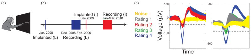
(a) A monkey performing the center-out reaching task on a fronto-parallel screen in complete darkness. (b) Timeline of the implantation and recording from Utah arrays. (c) A visual explanation of how waveforms are classified during spike sorting.
One array was implanted in PMd/M1 of each animal via standard neurosurgical techniques. The data were recorded using silicon ‘Utah’ arrays (Blackrock Technologies Inc., Salt Lake City, UT, USA) made up of 100 microelectrodes on a 10×10 grid with 400 μm center-to-center spacing. When data collection started, Monkey L and I’s arrays were 11 and 7 months old with substantial single unit activity. Data were recorded in the rig using a Cerebus system (Blackrock Microsystems, Salt Lake City, UT) over 6 and 8 weeks in monkeys L and I (Fig. 1b). Sixty-nine daily data sets were acquired during these time periods, but just 58 were analyzed because we only used data sets with over 100 reaches per target.
Blackrock’s built-in function was used for calculating the RMS voltage, which is slightly different than the standard calculation. Their algorithm calculates a biased estimate of the RMS voltage of the noise of the spike data stream. In the equations below, si represents the 30 kHz sampled spike stream after it is filtered, and xi represents the mean-squared value. Equation 1 calculates one VRMS value for a set of 600 continuous samples. It does this for two seconds, which results in 100 mean-squared values. In equation 2, the lowest five of these values are discarded and the next 20 are used to calculate the final RMS voltage. The rationale for this method is to avoid inflating the VRMS value due to the presence of large artifacts.
| (1) |
| (2) |
| (3) |
B. Spike Sorting Technique
We used the spike sorting methods described in [19,20,37] to visualize and identify the action potentials associated with different neurons. All neural data were analyzed offline in MATLAB (MathWorks, Natick, MA, USA). Although a closed-loop study is currently the gold standard, we performed an open-loop analysis because we wanted to analyze the same data using different techniques. Briefly, the data were high-pass filtered in order to eliminate local field fluctuations. When the signal crossed a threshold relative to its RMS voltage, a short voltage snippet was recorded before and after the threshold crossing. Very large “juicer” artifacts were also removed by eliminating “units” that stayed low for ~1ms after the triggering peak. These rare inter-trial events would not have impacted decoder performance, but were problematic for another study using this data that involved identifying the largest single unit [20]. Next, the remaining data were shifted in time in order to align all of the peaks. The data were then noise-whitened and the top four principle components of the waveform snippets were obtained. A mixture-of-gaussians model was fit to the data by a “relaxation” variant of Expectation-Maximization, which reduces the chances of converging to local maxima [19,37]. We manually rated the unit quality when forming our spike sorted data sets. The waveforms seen in every channel were categorized based on their shape, amplitude, and principal components (Fig. 1c). We classified waveforms as presumed single neurons (category “4”), single units with minimal contamination by other units (category “3”), and multi-units (category “2” or “1”). Category 1 units are likely contaminated by noise but still appear vaguely neural. Category 2 waveforms are more visibly neural, but they are depicted by a centroid that is not clearly delineated from the central “hash” in principal component analysis (PCA). When analyzing the principal components, category 3 waveforms have a clearly delineated centroid with some overlapping units in the outer ring. This unit categorization did not occur when creating the thresholded data sets. For thresholded data sets, all waveforms that surpassed a set threshold level were analyzed regardless of their apparent quality. The same electrodes were used in both analyses.
To demonstrate how decoder performance would change if action potentials were sorted using other sophisticated techniques, we also performed the unsupervised, wavelet spike sorting algorithm described by Quiroga et al [38]. Each spike was decomposed using a 4-level Haar wavelet transform. Next, ten wavelet coefficients with the largest deviations from normality were selected from each channel based on a modified Kolmogorov-Smirnov test. These were then clustered using the Potts Model superparamagnetic clustering (SPC) method. We used the software provided by Quiroga et al. to perform this analysis (www.vis.caltech.edu/~rodri/Wave_clus/Wave_clus_home.htm).
To detect neural units, we initially spike sorted each of the 96 channels using the automated wavelet sorting algorithm. Afterwards, we manually adjusted the parameters of the SPC to further improve our sort results based on visual inspection of the similarity of clustered waveforms. The SPC was constrained to yield no more than 8 clusters per channel, but the typical number of discerned clusters was 2–4. We applied this algorithm to the first day of recording in Monkey I and the first two days of recording in Monkey L.
C. Neural Data Analysis
The same two types of offline neural decoders used in [20] were also applied in this study. We used Naïve Bayes classification as a discrete neural decoder to calculate how accurately we could predict target selection [7]. We modeled the firing rate of each channel during a 500ms time window after target presentation as a Poisson distribution. The likelihood of each target was calculated using equations 4 and 5, where Θ is the actual target angle, θ is the predicted angle, yn is the number of spikes that occurred on neuron n, Y⃗ represents a vector of observed spikes, and N is the number of neurons.
| (4) |
| (5) |
The target that maximized this likelihood was selected. We trained and tested this model within the same day using 10-fold cross validation. We evaluated the performance using a percent correct variable that indicates how often we were able to correctly predict which target was selected.
In addition, we used a continuous offline linear decoder to predict the animal’s hand position [39]. For each trial, the data were divided into 100 ms bins and we found the average firing rate and hand position for every bin. We also used the firing rate information given at ten sequential 100 ms time lags. Using a linear Wiener filter, we modeled hand position as a function of firing rate for every channel. In equation 6, matrix X includes the average horizontal and vertical position for every bin. Every row of matrix Y contains the firing rates for each neuron at the 10 sequential time lags. Matrix B is calculated by linear regression and is the resulting linear decoder.
| (6) |
We trained and tested this model within the same day using 20-fold cross validation. Continuous performance is given using a correlation coefficient between predicted and actual hand position.
In order to validate the accuracy of the linear regression decoder, we also measured the “mean distance to the target” during a decoded reach and compared the two metrics in the threshold analyses. The mean distance to target metric represents the distance to the peripheral target averaged across all of the timesteps during the reach [40]. An optimal reach with uniform speed will have a mean distance to target equal to half the total distance.
III. Results
A. Neural Data Unit Quality and Performance
To ensure that the data we are analyzing is representative of common data sets, we evaluated several characteristics. Figure 2 displays the spike panels on day 1 for both animals and Table 1 gives the distribution of unit types. Both animals show a similar trend, in that most of the waveforms contain a mixture of multiple units and the fewest represent single units. For Monkey L, 40% percent of sorted waveforms are noisy category 1 waveforms and only 19% are single units. 47% percent of Monkey I’s waveforms are category 1 and only 12% are single units. These unit distributions are typical for a “good” array. Figure 3a displays the RMS voltages across all data sets. Monkey L’s average RMS voltage was 14.53 μVRMS and Monkey I’s was 9.22 μVRMS.
Figure 2.
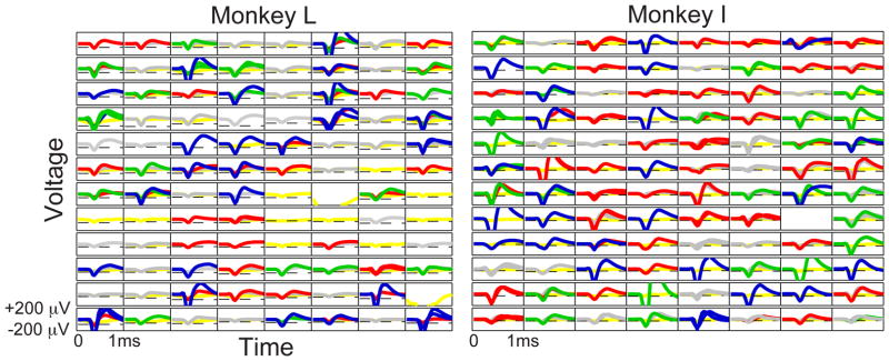
Spike panels of Monkey L (left) and I (right) on the first day of recording. Waveform colors correspond to the legend shown in Fig. 1c (single units are in blue, green waveforms represent single units with minimal contamination by other units, multi-units are in red, gray waveforms are multiple units with potential noise contamination, and noise is yellow). Sample thresholds are placed at −4.5*VRMS for Monkey L and −3*VRMS for Monkey I.
TABLE I.
Distribution of Waveforms on Day 1
| Category | Number of Waveforms | |
|---|---|---|
| Monkey L | Monkey I | |
| 1 | 60 (39.47%) | 102 (47.00%) |
| 2 | 39 (25.66%) | 59 (27.19%) |
| 3 | 24 (15.79%) | 31 (14.29%) |
| 4 | 29 (19.08%) | 25 (11.52%) |
Figure 3.

(a) Histograms of the RMS voltages across all electrode channels with firing rate >1Hz over all data sets. The black dot represents that animal’s mean RMS voltage. (b) We investigated how classes of waveforms performed individually, and then we combined waveform classes in order to determine which subset of spike sorted data would give the highest performance. Ratings of 4 represent single units and ratings of 1 contain a mixture of multiple units that is likely contaminated by noise. The gray error bars represent standard deviation.
Figure 3b displays both decoders’ performances when using different subsets of spike sorted data. When analyzing spike sorted data, channels with low firing rates were not removed. Because there were likely large low-firing units, performance was higher when they were included. Their presence ensured that we did not specifically disadvantage spike sorting when comparing it to thresholding. Category 2 waveforms, which likely correspond to multiple neurons, gave the highest performance when isolated and analyzed compared to other individual categories. In addition, the performance values when using categories 2 and 3 were only minimally improved when the single units were added into the analysis, though the improvements were statistically significant (t-tests, p<0.01). When units with ratings of 2 through 4 were analyzed, they demonstrated the best overall performance with the smallest standard deviation. The Naïve Bayes percent correct was 94% for Monkey L and 83% for Monkey I. Correlation coefficients were 0.94 (L) and 0.90 (I). This subset of spike sorted data is what we used as a comparison for the remaining analyses.
B. Best RMS Threshold for Decoding
It is common practice for researchers to use the RMS voltage to set a threshold [8,21,41,42]. To quantitatively determine the best placement, we tested the decoder performances of different threshold levels from −3*VRMS to −18*VRMS (Fig. 4a). Channels with a firing rate <1Hz were removed. For the Naïve Bayes decoder, the best threshold level was −4.5*VRMS for Monkey L and −3*VRMS for Monkey I. These thresholds produced Naïve Bayes percent correct values of 90% (L) and 89% (I), with chance≈14%. The best correlation coefficient was seen at −4*VRMS for Monkey L, giving ρ=0.92. For Monkey I, it was seen at −3*VRMS and produced ρ=0.89. We used the mean distance to target metric to corroborate the trends seen with correlation coefficient, and we found that both metrics displayed similar performance trends. Monkey L’s optimal threshold level was higher possibly because the array was older and may have contained more noise. For Monkey I, spike sorted data performance was slightly lower than that seen with threshold-crossing events. In addition, Monkey I’s threshold analyses did not contain a peak. The −3*VRMS threshold value, which was approximately −28μV on average, was initially set during recording and may not have been sufficiently low for this newer array. For Monkey L, the decoder performances of optimally thresholded data are only slightly lower than the spike sorted data, though the differences are statistically significant (p<0.001). For Monkey I, the Naïve Bayes performance of thresholded data is statistically significantly higher than that of the spike sorted data (p=2.4E-11), but the linear regression performance is not significantly different (p=0.908).
Figure 4.

On all figures, Monkey L is shown in blue and Monkey I is shown in red. The shaded region represents standard deviation. The dashed lines depict the decoder performance of the spike sorted data, specifically waveforms with ratings 2–4. This subset of data was previously found to give the highest sorted performance while likely ensuring that noise contamination is removed. (a) The top row demonstrates the performances of three decoders at varying VRMS threshold levels. (b) The bottom row represents the performance at varying fixed voltage threshold levels.
C. Best Fixed Voltage Threshold for Decoding
Some chip designs use a fixed voltage threshold for every channel instead of using the channels’ RMS voltages. This approach may work well if the mean and standard deviation of the RMS voltage are fairly tight. To test how our data sets would perform using this technique, and to determine which fixed voltage threshold would maximize performance, we tested the decoders for thresholds between −10 μV to −200 μV. Channels with a firing rate <1Hz were removed. The performances are given in the bottom row of Figure 4. For the Naïve Bayes decoder, Monkey L had the best performance at −70 μV, producing PC=88%. Monkey I was best at −10 μV, the lowest possible value, giving PC=89%. The best correlation coefficient was seen at −50 μV for Monkey L and −10 μV for Monkey I. This generated ρ=0.92 (L) and ρ=0.90 (I). The optimal thresholds in the linear regression analysis matched those seen in the mean distance to target analysis. For both animals, the performances associated with threshold levels of −10 to −30 μV were nearly identical due to the threshold level that was initially set during recording. For Monkey L, the performances of optimally thresholded data are only slightly lower than the spike sorted data, though the differences are statistically significant (p<0.001). For Monkey I, the Naïve Bayes performance of thresholded data is statistically significantly higher than that of the sorted data (p=2.7E-11), though the linear regression performance is not significantly different (p=0.912).
D. Partial Spike Sorting
If decoder performance is impaired when thresholding is used instead of spike sorting, it may be possible to spike sort a subset of the data to regain that performance. To determine which channels were best to spike sort, we tested the individual decoder performances of each channel on day 1. For every electrode, performance was measured when thresholded data were removed and replaced with the corresponding spike sorted data. We then ranked those channels by which ones gave the highest improvement [43] on day 1, and tested them on day 2 and beyond. We measured the performance after spike sorting the best channel, second best channel, etc. on the remaining data sets. For the partial spike sorting analysis, channels with low firing rates were not removed. The channels with low firing rates are different from day to day, which would interfere with our ability to rank and test the same electrodes. This analysis is primarily used as a tool to identify the channels in both animals that were most affected by spike sorting or thresholding.
Figure 5a demonstrates that as more electrodes were spike sorted, the decoder performances increased for Monkey L. These trends were anticipated based on our previous finding that sorted data outperformed thresholded data for this animal. The results from Monkey I are not displayed because the thresholded data outperformed sorted data, and this analysis is primarily focused on regaining performance lost during thresholding. If 26 of Monkey L’s channels were spike sorted, the linear regression performance was no longer statistically different than the fully spike sorted data (p = 0.06). After spike sorting only six channels, the correlation coefficient was within 1% of that seen when fully spike sorting. On the other hand, 76 channels had to be sorted until the achieved Naïve Bayes performance was not significantly different (p = 0.051). Spike sorting 61 channels brought the Naïve Bayes accuracy within 1% of the performance seen when fully spike sorting for Monkey L.
Figure 5.

(a) Decoder performance when a subset of channels is spike sorted and the remainder is thresholded at that animal’s optimal RMS threshold. In each graph, one solid line represents the performance when all channels are thresholded and the other line represents spike sorting all channels on day 2 and beyond. The data points in between the lines represent the performance seen when sorting a particular number of channels. (b) Decoder performance for each method of data processing. TC represents data that uses threshold-crossing events, WS symbolizes the wavelet sorted data, and SS characterizes the data sorted with our spike sorting algorithms.
When performing the partial spike sorting analysis, channels were ranked based on which gave the highest improvement in decoder performance on day 1 when its thresholded data was replaced with sorted data. In addition to the above analysis, we also analyzed the properties of the four best and worst channels to spike sort in both animals. As expected, the best channels to spike sort included multiple units with independent tuning properties. On the other hand, the worst channels to spike sort indicated that manual aspects of our spike sorting technique were occasionally flawed. For example, waveforms without a distinct bipolar shape were removed during spike sorting, yet they occasionally contained useful information. In addition, it is nearly impossible to visually distinguish between useful hash and noise. Two units could appear extremely similar, yet only one of them led to an improvement in decoder performance when spike sorted. Research by Wood and colleagues supports this claim, finding an average error rate of 23% false positive and 30% false negative regarding the manual sorting of synthetic data [28]. Finally, we found that the automated portion of our spike sorter occasionally broke a single good unit into multiple spikes, which may have made the signal noisier and less useful.
E. Wavelet-Based Spike Sorting
To fairly represent the performance of other spike sorting algorithms, we performed an unsupervised, wavelet spike sorting algorithm [38]. Unlike principal component analysis (PCA), wavelet coefficients offer better discrimination of the temporal features of action potentials due to the time scaling property of the wavelet decomposition. Moreover, superparamagnetic clustering (SPC) offers a more general clustering method, neither requiring non-overlapping clusters in the feature space, nor assuming a particular distribution (such as our original Gaussian Expectation-Maximization clustering method) [38]. We tested the wavelet-sorted algorithm on three data sets to ensure a good approximation. As Figure 5b demonstrates, the differences in decoder performance between the wavelet-sorted data and our PCA-clustered data are very small. Therefore, we concluded that it was acceptable to perform PCA-based spike sorting methods in our analyses.
IV. Discussion
We have demonstrated that threshold-crossing events can be used to analyze BMI data instead of spike sorting without causing a substantial decrease in performance. The Naïve Bayes percent correct changed by 5% on average and the correlation coefficient changed by 0.015. Based on the quality and performance of our neural data, it appears that it is representative of that commonly seen for BMIs. Our results demonstrate that thresholds between −3 to −5*VRMS result in similar performances. While this study contains a limited number of arrays, we hypothesize that the best RMS threshold to place for arrays with smaller noise is around −3*VRMS. For arrays with larger noise, the best threshold may be approximately −4.5*VRMS. It is not possible to determine a fixed voltage threshold that will work on every data set, because characteristics vary between subjects. A fixed voltage threshold generally gives lower performance and also requires the user to manually tune the threshold.
The decoder performances of Monkey L’s data are indicative of the common notion that spike sorted data performance is slightly higher than that of thresholded data, although the Naïve Bayes accuracy is only 4% greater and the correlation coefficient is just 0.02 higher. While it still requires human intervention, our partial spike sorting analysis demonstrates that any performance lost due to thresholding can be regained after spike sorting a small subset of channels. The waveform characteristics of the best and worst channels to sort did not display any consistent trends, so it is not possible for us to say exactly which traits to look for when choosing a subset of channels to spike sort. Although spike sorting was favorable when there were multiple units with independent tuning properties, tuning properties cannot be determined upon inspection only. In addition, it is nearly impossible to visually distinguish between useful hash and noise. An algorithm by Ventura [44] would be useful in a partial spike sorting analysis, because it determines if units should be unsorted or sorted based on what leads to the highest decoder performance.
On the other hand, the spike sorted and thresholded data in Monkey I showed dissimilar results. The correlation coefficient was not significantly different. In addition, for Naïve Bayes classification, the thresholded data performance was actually higher than that of sorted data. This is possibly due to unnecessary unit splitting by the automated portion of the spike sorter.
Opposite results between two animals also occurred in a study performed by Fraser and colleagues, where spike sorted data outperformed unsorted data in one case but not the other [21]. Our results are consistent with the studies by Gilja et al. and Stark and Abeles, in that we demonstrate that complex movements can be decoded without the detection of spikes [8,24]. However, the recent study published by Todorova et al. concluded that spike sorting adds value to the threshold-crossing methods employed in BMI decoding [27]. In their study, threshold levels were set in order to maximize the ability to perform spike sorting in Monkey A. Their Figure 2 shows that many of the thresholds for this animal were higher in amplitude than the optimal levels we saw, which would tend to hinder the decoder performance of thresholded data (as seen in our Figure 4). They demonstrated that the optimal linear estimator (OLE) amplitude-sorted data from Monkey A led to ~12% performance gain compared to OLE unsorted data. In our study, with Monkey L, a threshold of −6.5*VRMS can also cause the sorted data to outperform thresholded data by 12%. The data from the other animal in their study was thresholded at three standard deviations below the mean of the bandpass filtered voltage traces, which led to threshold levels more similar to ours. Subsequently, the OLE amplitude-sorted data only outperformed OLE unsorted data by ~6%, which was more consistent with Monkey L’s results from our study. Our study concludes that if you sweep the threshold systematically, it is possible to find a range where threshold crossings perform essentially as well as spike sorting. The use of threshold crossings instead of spike sorting will make it easier to build implantable prosthetics processors and chips with threshold-crossing detectors [45].
It is important to note that our analysis was performed offline, and our sorting method was not fully automated. Other studies, such as that by Todorova et al., found similar results across more decoders. Our conclusions do not hold if there is a large amount of noise or motion artifacts, although it is rare for these to hinder threshold crossings while leaving units intact. In fact, noise artifacts tend to be lower in wireless systems that often have very short wires and good shielding [45]. To our knowledge, this is the first study to determine an optimal threshold level in addition to analyzing the contributions of different neuron subpopulations in a large number of data sets.
With current microelectrode array technology, our study demonstrates that thresholding and spike sorting can be used essentially interchangeably without seeing a significant decrease in performance. The utilization of threshold-crossing events may allow for an easier transition of BMI devices from research into the clinic due to simpler hardware and software. This also allows for long-term systems with lower power consumption and it can be applied to systems with a high number of electrode channels.
Acknowledgments
This work was supported by National Science Foundation graduate research fellowships (CAC, VG), NDSEG Fellowship (VG), Texas Instruments Stanford Graduate Fellowship (JF), Burroughs Wellcome Fund Career Awards in the Biomedical Sciences (KVS), the Christopher Reeve Paralysis Foundation (SIR, KVS), a Stanford University Graduate Fellowship (CAC), a Stanford NIH Medical Scientist Training Program grant and Soros Fellowship (PN) and the following awards to KVS: Stanford CIS, Sloan Foundation, NIH CRCNS R01-NS054283, McKnight Endowment Fund for Neuroscience, NIH Director’s Pioneer Award DP1HD075623, DARPA Revolutionizing Prosthetics program contract N66001-06-C-8005, and DARPA REPAIR contract N66001-10-C-2010.
References
- 1.Wolpaw JR, Birbaumer N, McFarland DJ, Pfurtscheller G, Vaughan TM. Brain–computer interfaces for communication and control. Clin Neurophysiol. 2002 Jun;113(6):767–791. doi: 10.1016/s1388-2457(02)00057-3. [DOI] [PubMed] [Google Scholar]
- 2.Schwartz AB. CORTICAL NEURAL PROSTHETICS. Annu Rev Neurosci. 2004 Jul;27(1):487–507. doi: 10.1146/annurev.neuro.27.070203.144233. [DOI] [PubMed] [Google Scholar]
- 3.Serruya MD, Hatsopoulos NG, Paninski L, Fellows MR, Donoghue JP. Brain-machine interface: Instant neural control of a movement signal. Nature. 2002;416(6877):141–142. doi: 10.1038/416141a. [DOI] [PubMed] [Google Scholar]
- 4.Taylor DM. Direct Cortical Control of 3D Neuroprosthetic Devices. Science. 2002 Jun;296(5574):1829–1832. doi: 10.1126/science.1070291. [DOI] [PubMed] [Google Scholar]
- 5.Carmena JM, Lebedev MA, Crist RE, O’Doherty JE, Santucci DM, Dimitrov DF, Patil PG, Henriquez CS, Nicolelis MAL. Learning to Control a Brain–Machine Interface for Reaching and Grasping by Primates. PLoS Biol. 2003;1(2):e2. doi: 10.1371/journal.pbio.0000042. [DOI] [PMC free article] [PubMed] [Google Scholar]
- 6.Musallam S. Cognitive Control Signals for Neural Prosthetics. Science. 2004 Jul;305(5681):258–262. doi: 10.1126/science.1097938. [DOI] [PubMed] [Google Scholar]
- 7.Santhanam G, Ryu SI, Yu BM, Afshar A, Shenoy KV. A high-performance brain–computer interface. Nature. 2006 Jul;442(7099):195–198. doi: 10.1038/nature04968. [DOI] [PubMed] [Google Scholar]
- 8.Gilja V, Nuyujukian P, Chestek CA, Cunningham JP, Yu BM, Fan JM, Churchland MM, Kaufman MT, Kao JC, Ryu SI, Shenoy KV. A high-performance neural prosthesis enabled by control algorithm design. Nat Neurosci. 2012 Nov;15(12):1752–1757. doi: 10.1038/nn.3265. [DOI] [PMC free article] [PubMed] [Google Scholar]
- 9.Hochberg LR, Serruya MD, Friehs GM, Mukand JA, Saleh M, Caplan AH, Branner A, Chen D, Penn RD, Donoghue JP. Neuronal ensemble control of prosthetic devices by a human with tetraplegia. Nature. 2006 Jul;442(7099):164–171. doi: 10.1038/nature04970. [DOI] [PubMed] [Google Scholar]
- 10.Kennedy PR, Bakay RA, Moore MM, Adams K, Goldwaithe J. Direct control of a computer from the human central nervous system. Rehabil Eng IEEE Trans On. 2000;8(2):198–202. doi: 10.1109/86.847815. [DOI] [PubMed] [Google Scholar]
- 11.Leuthardt EC, Schalk G, Wolpaw JR, Ojemann JG, Moran DW. A brain–computer interface using electrocorticographic signals in humans. J Neural Eng. 2004 Jun;1(2):63–71. doi: 10.1088/1741-2560/1/2/001. [DOI] [PubMed] [Google Scholar]
- 12.Patil PG, Carmena JM, Nicolelis MAL, Turner DA. Ensemble recordings of human subcortical neurons as a source of motor control signals for a brain-machine interface. Neurosurgery. 2004 Jul;55(1):27–35. discussion 35–38. [PubMed] [Google Scholar]
- 13.Velliste M, Perel S, Spalding MC, Whitford AS, Schwartz AB. Cortical control of a prosthetic arm for self-feeding. Nature. 2008 Jun;453(7198):1098–1101. doi: 10.1038/nature06996. [DOI] [PubMed] [Google Scholar]
- 14.Collinger JL, Wodlinger B, Downey JE, Wang W, Tyler-Kabara EC, Weber DJ, McMorland AJ, Velliste M, Boninger ML, Schwartz AB. High-performance neuroprosthetic control by an individual with tetraplegia. The Lancet. 2013;381(9866):557–564. doi: 10.1016/S0140-6736(12)61816-9. [DOI] [PMC free article] [PubMed] [Google Scholar]
- 15.Hochberg LR, Bacher D, Jarosiewicz B, Masse NY, Simeral JD, Vogel J, Haddadin S, Liu J, Cash SS, van der Smagt P, Donoghue JP. Reach and grasp by people with tetraplegia using a neurally controlled robotic arm. Nature. 2012 May;485(7398):372–375. doi: 10.1038/nature11076. [DOI] [PMC free article] [PubMed] [Google Scholar]
- 16.Georgopoulos AP, Kalaska JF, Caminiti R, Massey JT. On the relations between the direction of two-dimensional arm movements and cell discharge in primate motor cortex. J Neurosci. 1982;2(11):1527–1537. doi: 10.1523/JNEUROSCI.02-11-01527.1982. [DOI] [PMC free article] [PubMed] [Google Scholar]
- 17.Evarts EV. Pyramidal tract activity associated with a conditioned hand movement in the monkey. J Neurophysiol. 1966 Nov;29(6):1011–1027. doi: 10.1152/jn.1966.29.6.1011. [DOI] [PubMed] [Google Scholar]
- 18.Lewicki MS. [Accessed: 31-Mar-2014];A review of methods for spike sorting: the detection and classification of neural action potentials. 2009 Jul 09; [Online]. Available: http://informahealthcare.com/doi/abs/10.1088/0954-898X_9_4_001. [PubMed]
- 19.Santhanam G, Sahani M, Ryu SI, Shenoy KV. An extensible infrastructure for fully automated spike sorting during online experiments. Engineering in Medicine and Biology Society, 2004. IEMBS’04. 26th Annual International Conference of the IEEE; 2004. pp. 4380–4384. [DOI] [PubMed] [Google Scholar]
- 20.Chestek CA, Gilja V, Nuyujukian P, Foster JD, Fan JM, Kaufman MT, Churchland MM, Rivera-Alvidrez Z, Cunningham JP, Ryu SI, Shenoy KV. Long-term stability of neural prosthetic control signals from silicon cortical arrays in rhesus macaque motor cortex. J Neural Eng. 2011 Aug;8(4):045005. doi: 10.1088/1741-2560/8/4/045005. [DOI] [PMC free article] [PubMed] [Google Scholar]
- 21.Fraser GW, Chase SM, Whitford A, Schwartz AB. Control of a brain–computer interface without spike sorting. J Neural Eng. 2009 Oct;6(5):055004. doi: 10.1088/1741-2560/6/5/055004. [DOI] [PubMed] [Google Scholar]
- 22.Zumsteg ZS, Kemere C, O’Driscoll S, Santhanam G, Ahmed RE, Shenoy KV, Meng TH. Power Feasibility of Implantable Digital Spike Sorting Circuits for Neural Prosthetic Systems. IEEE Trans Neural Syst Rehabil Eng. 2005 Sep;13(3):272–279. doi: 10.1109/TNSRE.2005.854307. [DOI] [PubMed] [Google Scholar]
- 23.Dethier J, Nuyujukian P, Ryu SI, Shenoy KV, Boahen K. Design and validation of a real-time spiking-neural-network decoder for brain–machine interfaces. J Neural Eng. 2013 Jun;10(3):036008. doi: 10.1088/1741-2560/10/3/036008. [DOI] [PMC free article] [PubMed] [Google Scholar]
- 24.Stark E, Abeles M. Predicting Movement from Multiunit Activity. J Neurosci. 2007 Aug;27(31):8387–8394. doi: 10.1523/JNEUROSCI.1321-07.2007. [DOI] [PMC free article] [PubMed] [Google Scholar]
- 25.Scherberger H, Jarvis MR, Andersen RA. Cortical Local Field Potential Encodes Movement Intentions in the Posterior Parietal Cortex. Neuron. 2005 Apr;46(2):347–354. doi: 10.1016/j.neuron.2005.03.004. [DOI] [PubMed] [Google Scholar]
- 26.Wang D, Zhang Q, Li Y, Wang Y, Zhu J, Zhang S, Zheng X. Long-term decoding stability of local field potentials from silicon arrays in primate motor cortex during a 2D center out task. J Neural Eng. 2014 Jun;11(3):036009. doi: 10.1088/1741-2560/11/3/036009. [DOI] [PubMed] [Google Scholar]
- 27.Todorova S, Sadtler P, Batista A, Chase S, Ventura V. To sort or not to sort: the impact of spike-sorting on neural decoding performance. J Neural Eng. 2014 Oct;11(5):056005. doi: 10.1088/1741-2560/11/5/056005. [DOI] [PMC free article] [PubMed] [Google Scholar]
- 28.Wood F, Black MJ, Vargas-Irwin C, Fellows M, Donoghue JP. On the Variability of Manual Spike Sorting. IEEE Trans Biomed Eng. 2004 Jun;51(6):912–918. doi: 10.1109/TBME.2004.826677. [DOI] [PubMed] [Google Scholar]
- 29.Markowitz DA, Wong YT, Gray CM, Pesaran B. Optimizing the Decoding of Movement Goals from Local Field Potentials in Macaque Cortex. J Neurosci. 2011 Dec;31(50):18412–18422. doi: 10.1523/JNEUROSCI.4165-11.2011. [DOI] [PMC free article] [PubMed] [Google Scholar]
- 30.Bansal AK, Truccolo W, Vargas-Irwin CE, Donoghue JP. Decoding 3D reach and grasp from hybrid signals in motor and premotor cortices: spikes, multiunit activity, and local field potentials. J Neurophysiol. 2012 Mar;107(5):1337–1355. doi: 10.1152/jn.00781.2011. [DOI] [PMC free article] [PubMed] [Google Scholar]
- 31.Flint RD, Lindberg EW, Jordan LR, Miller LE, Slutzky MW. Accurate decoding of reaching movements from field potentials in the absence of spikes. J Neural Eng. 2012 Aug;9(4):046006. doi: 10.1088/1741-2560/9/4/046006. [DOI] [PMC free article] [PubMed] [Google Scholar]
- 32.Flint RD, Ethier C, Oby ER, Miller LE, Slutzky MW. Local field potentials allow accurate decoding of muscle activity. J Neurophysiol. 2012 Jul;108(1):18–24. doi: 10.1152/jn.00832.2011. [DOI] [PMC free article] [PubMed] [Google Scholar]
- 33.Flint RD, Wright ZA, Scheid MR, Slutzky MW. Long term, stable brain machine interface performance using local field potentials and multiunit spikes. J Neural Eng. 2013 Oct;10(5):056005. doi: 10.1088/1741-2560/10/5/056005. [DOI] [PMC free article] [PubMed] [Google Scholar]
- 34.Mehring C, Rickert J, Vaadia E, de Oliveira SC, Aertsen A, Rotter S. Inference of hand movements from local field potentials in monkey motor cortex. Nat Neurosci. 2003 Dec;6(12):1253– 1254. doi: 10.1038/nn1158. [DOI] [PubMed] [Google Scholar]
- 35.Zhuang J, Truccolo W, Vargas-Irwin C, Donoghue JP. Decoding 3-D Reach and Grasp Kinematics From High-Frequency Local Field Potentials in Primate Primary Motor Cortex. IEEE Trans Biomed Eng. 2010 Jul;57(7):1774–1784. doi: 10.1109/TBME.2010.2047015. [DOI] [PMC free article] [PubMed] [Google Scholar]
- 36.Hwang EJ, Andersen RA. The utility of multichannel local field potentials for brain–machine interfaces. J Neural Eng. 2013 Aug;10(4):046005. doi: 10.1088/1741-2560/10/4/046005. [DOI] [PMC free article] [PubMed] [Google Scholar]
- 37.Sahani M. Latent Variable Models for Neural Data Analysis. California Institute of Technology; 1999. [Google Scholar]
- 38.Quiroga R, Nadasdy Z, Ben-Shaul Y. Unsupervised Spike Detection and Sorting with Wavelets and Superparamagnetic Clustering. Neural Comput. 2004 Aug;16(8):1661–1687. doi: 10.1162/089976604774201631. [DOI] [PubMed] [Google Scholar]
- 39.Rao YN, Kim S-P, Sanchez JC, Erdogmus D, Principe JC, Carmena JM, Lebedev MA, Nicolelis MA. Learning mappings in brain machine interfaces with echo state networks. IEEE International Conference on Acoustics, Speech, and Signal Processing, 2005. Proceedings. (ICASSP’05); 2005. pp. v/233–v/236. [Google Scholar]
- 40.Cunningham JP, Nuyujukian P, Gilja V, Chestek CA, Ryu SI, Shenoy KV. A closed-loop human simulator for investigating the role of feedback control in brain-machine interfaces. J Neurophysiol. 2011 Apr;105(4):1932–1949. doi: 10.1152/jn.00503.2010. [DOI] [PMC free article] [PubMed] [Google Scholar]
- 41.Gilja V, Pandarinath C, Blabe CH, Hochberg LR, Shenoy KV, Henderson JM. Program No. 80.06.2013. San Diego, CA: 2013. Design and application of a high performance intracortical brain computer interface for a person with amyotrophic lateral sclerosis. [Google Scholar]
- 42.Pandarinath C, Gilja V, Blabe C, Jarosiewicz B, Perge JA, Hochberg LR, Shenoy KV, Henderson JM. High-performance communication using neuronal ensemble recordings from the motor cortex of a person with ALS. presented at the American Society for Stereotactic and Functional Neurosurgery; Washington, D.C. 2014. [Google Scholar]
- 43.Fan JM, Nuyujukian P, Kao JC, Chestek CA, Ryu SI, Shenoy KV. Intention estimation in brain–machine interfaces. J Neural Eng. 2014 Feb;11(1):016004. doi: 10.1088/1741-2560/11/1/016004. [DOI] [PMC free article] [PubMed] [Google Scholar]
- 44.Ventura V. Spike train decoding without spike sorting. Neural Comput. 2008;20(4):923–963. doi: 10.1162/neco.2008.02-07-478. [DOI] [PMC free article] [PubMed] [Google Scholar]
- 45.Chestek C, Gilja V, Nuyujukian P, Kier RJ, Solzbacher F, Ryu S, Harrison RR, Shenoy KV. HermesC: Low-Power Wireless Neural Recording System for Freely Moving Primates. IEEE Trans Neural Syst Rehabil Eng. 2009 Aug;17(4):330–338. doi: 10.1109/TNSRE.2009.2023293. [DOI] [PubMed] [Google Scholar]