Zen and the Art of Multiple Comparisons

Abstract

The need for appropriate multiple comparisons correction when performing statistical inference is not a new problem. However, it has come to the forefront in many new modern data-intensive disciplines. For example, researchers in areas such as imaging and genetics are routinely required to simultaneously perform thousands of statistical tests. Ignoring this multiplicity can cause severe problems with false positives, thereby introducing non-reproducible results into the literature. This article serves as an introduction to hypothesis testing and multiple comparisons for practical research applications, with a particular focus on its use in the analysis of functional magnetic resonance imagining (fMRI) data. We will discuss hypothesis testing and a variety of principled techniques for correcting for multiple tests. We also illustrate potential pitfalls and problems that can occur if the multiple comparisons issue is not dealt with properly. We conclude by discussing effect size estimation, an issue often linked with the multiple comparisons problem.

1. Introduction

In a number of modern scientific research disciplines the analysis of large data sets has become increasingly common, leading to an explosion in the amount of available data. This increase has profoundly changed the manner in which many aspects of statistical analysis are performed. One such example is how statistical tests are conducted, especially with regards to correcting for multiple comparisons. While the idea of correcting for multiple comparisons in not new per se, the need to correct for tens of thousands of tests is a very recent problem. For example, one may be interested in testing tens of thousands of features in a genome-wide study against some null hypothesis, or in attempting to detect brain activation across a hundred thousand brain regions. Not appropriately correcting for multiple comparisons can cause severe problems with regards to false positives. This in turn, can lead to spurious findings being introduced into the literature, which according to several recent high-profile studies is reaching epidemic levels (1,2).

This article serves as an introduction to the fundamental ideas behind hypothesis testing and the principled control for multiple comparisons. We will discuss a variety of techniques for correcting for multiple tests that are commonly used in modern applications, such as economics, genetics and imaging. We will seek to contrast the various methods and highlight potential consequences of not dealing with the problem appropriately. In particular, we will attempt to illustrate the problem by focusing on the analysis of functional magnetic resonance imaging (fMRI) data as a motivating example. Finally, we will discuss the issue in relation to the study of individual differences and effect size reporting in neuroimaging studies. However, we begin by formulating the problem.

Hypothesis Testing

Hypothesis tests are perhaps the most commonly used statistical inference technique. They are used to assess evidence provided by the data in favor of some claim about the population. For example, they have found wide usage in determining whether a certain drug works better than a placebo, to detect genes that show differential expression across two or more biological conditions, or to determine whether a particular brain region shows significant activation (3,4,5).

The goal of a hypothesis test is to determine whether there is sufficient evidence to reject the null hypothesis H₀ about a population parameter (often a statement of no effect), in favor of an alternative hypothesis H_a. After stating the null and alternative hypothesis, the second step is to calculate a test statistic, which measures the compatibility of the data and the null hypothesis. Typically test statistics are designed so that small values indicate consistency with H₀ and large values inconsistency. The latter implies either that the null hypothesis is true and we have simply observed an unusual set of data, or that the null hypothesis is false and should be rejected. Making this determination is critical towards addressing the problem at hand.

In order to determine what constitutes an unusually large test statistic, the third step is to calculate the p-value, which represents the probability that the statistic would take a value as or more extreme than that actually observed under the assumption that the null hypothesis is true. A small p-value indicates that we have observed an unusual observation under H₀, and calls the null hypothesis into doubt.

The fourth, and final, step is to assess statistical significance. That is, to determine whether or not to reject H₀. In order to make this determination, we sometimes compare the p-value with some fixed value α that we regard as decisive. For example, choosing α=0.05 implies that we would reject H₀ if we observed a test statistic so extreme that it would occur less than once out of every 20 times this particular test were performed if the null hypothesis were true.

As an alternative one can instead assess whether or not the observed test statistic is greater than a fixed threshold u_α, where u_α represents the value the test statistic would take if its p-value were exactly equal to α. Mathematically, we write that threshold u_α controls the false positive rate at level α = P(T > u_α∣H₀), where T is the test statistic.

To set the stage for the remaining text on multiple testing, we briefly review here that the two types of error in statistical significance testing are referred to as Type I and Type II errors. The former occurs when H₀ is true, but we mistakenly reject it. This is also referred to as a false positive, and its probability is controlled by the significance level α. The latter occurs when H₀ is false, but we fail to reject it. This is also referred to as a false negative. The probability of a true negative is the power of the test.

In general, it is desirable to choose a threshold that makes the likelihood of observing a Type I error as small as possible. However, this has a detrimental effect on power. In the most extreme case we may chose to never reject H₀, which would lead to a zero Type I error rate but have the opposite effect on the Type II error rate. Hence, the choice of an appropriate threshold is a delicate balance between sensitivity (true positive rate) and specificity (true negative rate). In practice, researchers typically choose a threshold that controls the Type I error and thereafter seek alternative ways to control the Type II error. For example, by taking a larger sample size one can decrease the uncertainty related to the parameter estimate and thereby reduce the likelihood of making a Type II error.

The Multiple Comparisons Problem

As mentioned above, in modern applications we often need to perform multiple hypothesis tests at the same time, including in imaging when we perform hypothesis tests simultaneously over many areas of the brain in order to determine which are significant, or in genetics when we seek to test thousands of features in a genome-wide study against some null hypothesis. In these situations choosing an appropriate hypothesis testing threshold is complicated by the fact that we are dealing with a family of tests.

If more than one α-level hypothesis test is performed, the risk of making at least one Type I error will exceed α. For example, if two independent tests are performed, each at α-level equal to 0.05, then the probability that neither test gives rise to a Type I error is equal to (1-0.05)² = 0.9025. Hence, the probability of at least one Type I error will be greater than 0.05.

As the number of tests increases, so does the likelihood of getting at least one false positive. In the case when we are performing m independent tests at α=0.05, the likelihood of observing at least one false positive is 1-(0.95)^m, which very quickly approaches 1 as m becomes large, nearly guaranteeing that, without correction, at least one false positive will occur. In fact, at α-level equal to 0.05, we would expect to observe 5 false positives for every 100 tests performed.

This example illustrates that methods used to threshold a test statistic in a single test are woefully inadequate for dealing with families consisting of many tests. The question then becomes how to choose an appropriate threshold that provides adequate control over the number of false positives. If the chosen threshold is too conservative, we risk losing the power to detect meaningful results. If instead the threshold is too liberal, this will result in an excessive number of false positives. This paper discusses a variety of methods designed to control the number of false positives while avoiding excessive loss of power. But before we start, we will illustrate the problem in the context of fMRI data.

2. Multiple Comparisons in Neuroimaging

Functional magnetic resonance imaging (fMRI) is a non-invasive technique for studying brain activity. For a detailed description of this technique see Wager et al. (6) or Lindquist (7). During the course of an fMRI experiment, a series of three-dimensional brain volumes are acquired while the subject performs a set of tasks. Each volume consists of roughly 100,000 uniformly spaced volume elements (voxels) that partition the brain into equally sized boxes. Each voxel corresponds to a spatial location and has a number associated with it that represents its intensity, which is related to the spatial distribution of the nuclear spin density in that location. During the course of an fMRI experiment, several hundred volumes of this type are acquired. Intensity values from each individual voxel can be extracted to create a time series whose length corresponds to the number of acquired images.

The most common use of fMRI data is to detect areas of the brain that activate in response to a specific task. Typically, data analysis is performed using the so-called “massive univariate approach”, where a separate model is constructed and fit to data from each voxel. Hence, a separate hypothesis test is performed at every voxel of the brain in order to determine whether activation in that voxel is significantly different from zero. The results of these tests are summarized in a statistical image, such as the one shown in Fig. 1. These maps illustrate the test statistic value (e.g. t-statistic) at every voxel of the brain. This particular example corresponds to a two-dimensional image with dimensions 79×95 (i.e., consisting of 7,505 voxels), with one test performed at each voxel.

Figure 1.

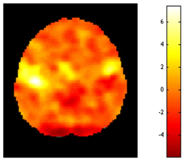
An example of a statistical image. Separate hypotheses tests are performed at each voxel of the brain to determine whether activation in that voxel is significantly different from zero. The results of these tests are summarized in a statistical image showing the value of the test statistic at each voxel.

The final results of fMRI studies are often summarized as a set of ‘activated regions’ superimposed on an anatomical brain image, such as those shown in Fig. 2. These types of summaries describe brain activation by color-coding voxels whose test statistic exceeds a certain statistical threshold for significance. The implication is that these voxels were activated by the experimental task. In many fields, test statistics whose p-values are below 0.05 are considered sufficient evidence to reject the null hypothesis. In brain imaging, however, on the order of 100,000 hypothesis tests are typically performed at a single time. Hence, using a voxel-wise α of 0.05 means that roughly 5% of the voxels will show false positive results. This implies that we would actually expect on the order of 5,000 false positive results! Thus, even if a certain experimental task does not produce a true activation, there is still a good chance that without an appropriate correction for multiple comparisons, the resulting activation map will show a number of activated regions, which would lead to erroneous conclusions and the potential for false positives to be introduced into the literature.

Figure 2.

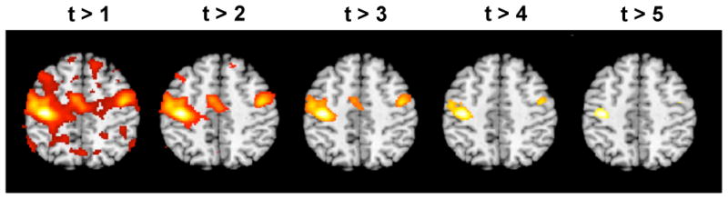
An example of a series of thresholded statistical images. The statistical image shown in Fig. 1 was thresholded using five different values, and voxels deemed significant are color-coded and superimposed onto an anatomical image. Clearly the choice of threshold will have a large impact on which voxels are deemed active.

A critical decision is therefore the choice of an appropriate threshold to use in deciding whether voxels are ‘active.’ Fig. 2 shows how changing the threshold provides substantially different conclusions about which regions are active in the brain. Using a more lenient threshold provides results similar to the ones seen on the left-hand side of Fig. 2. Here we expect to detect all the truly active voxels, but would have strong concerns that a large portion of the voxels deemed active were in fact false positives. In contrast, using a more stringent threshold we would obtain results similar to the ones seen on the right-hand side of Fig. 2. Here we are fairly certain that the voxels deemed active are true positives. However, it appears likely that we may have a large number of voxels that are false negatives, i.e. should have been rejected but weren't. Clearly some intermediate threshold between these two extremes should be chosen, but the exact value is not immediately evident. A principled approach towards correcting for multiple comparisons is clearly needed.

3. Controlling for Multiple Comparisons

The first step in controlling for multiple comparisons is to quantify the likelihood of obtaining false positives. We focus on two such metrics, namely the family-wise error rate (FWER), defined as the probability of obtaining at least one false positive in a family of tests, and the false discovery rate (FDR), defined as the proportion of false positives among all rejected tests. In the following sections we will explore a number of approaches that control each of these rates and will attempt to describe fundamental differences between the FWER and FDR. In particular, we will illustrate their use in the context of the analysis of fMRI data described in the previous section, and we will use the language of this field to describe the methods.

3.1 FWER

The FWER is defined as the probability of making one or more Type I errors in a family of tests, under the null hypothesis. This implies that in a family of m tests we want to limit the probability that any of them results in a false positive. Hence, FWER controlling procedures provide very stringent control over false positives, with thresholds closer to those seen in the right-hand side of Fig. 2. However, as we will see using such a stringent threshold has its cost with respect to power and the ability to detect true effects.

There exist a number of popular FWER controlling methods, including Bonferroni correction, random field theory, and permutation tests. We briefly discuss each of these methods below, as they are the most commonly used ones in the neuroimaging context, but we begin by first defining some notation and providing two ways of expressing the FWER.

Let H_0i be the hypothesis that there is no activation in voxel i, where i = 1,…,m. Here m represents the total number of voxels. Let T_i be the value of the test statistic at voxel i. The family-wise null hypothesis, H₀, states that there is no activation in any of the m voxels. Mathematically, this can be expressed as $H_0=\underset{i}{\cap }{H}_{0i}$. In words, for H₀ to be true, all of the individual H_0i must be true. Hence, if we were to reject a single null hypothesis, H_0i, we would also reject the family-wise null hypothesis. For these reasons, a false positive at any voxel would give rise to a family-wise error (FWE).

Assuming H₀ is true, we want the probability of falsely rejecting H₀, or falsely rejecting any of the m tests, to be controlled by some fixed value α. This is represented by the following mathematical expression:

$$\mathit{\text{FWER}}=P\left(\underset{i}{\cup }\{T_i\ge u_{\alpha }\}|H_0\right)\le \alpha .$$ [1]

In words, the FWER represents the probability under the null hypothesis that any of the m test statistics T_i take values above a given threshold, and thus give rise to a false positive. Our goal is to determine a threshold u_α, such that the inequality above holds.

As an alternative, we can express the FWER in terms of the maximum test statistic. Note that the probability that any test statistic exceeds u_α under the null hypothesis is equivalent to the probability that the maximum test statistic exceeds u_α under the null. Hence, an alternative approach to controlling the FWER is to choose the threshold u_α such that the maximum statistic only exceeds it with probability α under the null hypothesis. However, this necessitates knowing the distribution of the maximum statistic under the null. This is not always self-evident, and several of the methods discussed below attempt to approximate this distribution.

Bonferroni Correction

The most common approach towards dealing with multiple comparisons is Bonferroni correction. Here the value of α that is used to determine the threshold u_α for each individual test is divided by m, the total number of statistical tests performed. Hence, for a given value of α and m we choose u_α so that:

$$P(T_i\ge u_{\alpha }|H_0)\le \frac{\alpha }{m}.$$ [2]

This provides an extremely stringent threshold for each individual test. For example, if we want to control the FWER at α=0.05 and are performing 1,000 tests, than we would choose a threshold corresponding to an α-level of 0.00005 for each individual test. For a two-sided Z-test this corresponds to raising the threshold u_α from 1.96 to 4.06, which substantially increases the amount of evidence required to reject a null hypothesis.

To see how this choice controls the FWER we make use of Boole's inequality, which states that

$$P({\cup }_i\left\{T_i\ge u\right\}|H_0)\le {\sum }_{i}P(T_i\ge u|H_0).$$ [3]

In words, this inequality states that the probability of at least one test being significant under the null hypothesis is no larger than the sum of the probabilities of all of the tests being significant. Using this result it follows that

$$\mathit{\text{FWER}}\le {\sum }_{i}P(T_i\ge u|H_0)\le {\sum }_i\frac{\alpha }{m}=\alpha .$$ [4]

Thus, using Bonferroni correction we are guaranteed to control the FWER at level α.

The Bonferroni correction, though intuitive and simple to use, tends to be very conservative, i.e. results in very strict significance levels. Therefore, it ultimately decreases the power of the test and greatly increases the chance of obtaining false negatives. These problems are particularly evident for correlated data, such as fMRI data, which has significant spatial correlation since neighboring voxels exhibit similar behavior. Hence, it is generally not considered optimal for use with fMRI data.

Random Field Theory

In the fMRI community, random field theory (RFT) (8) is the most popular approach for controlling the FWER. Theoretically, it is considerably more complicated than the Bonferroni Correction and full understanding of the approach is beyond the scope of this paper.

In short, the image of voxel-wise test statistic values are assumed to be a discrete sampling of a continuous smooth random field. The RFT approach uses information about the smoothness of the image and a property called the Euler characteristic to determine the appropriate threshold. The smoothness of the image is expressed in terms of resolution elements, or resels, which is roughly equivalent to the number of independent comparisons. For a two-dimensional image the number of resels can be computed as

$$R=\frac{V}{{\mathit{\text{FWHM}}}_x{\mathit{\text{FWHM}}}_y},$$ [5]

where V represents the volume of the search region (i.e., the number of voxels) and the full width at half maximum (FWHM) values represent the estimated smoothness in each direction of the image. As the smoothness of the image increase, so do the FWHM values, and the resel count decreases.

The Euler characteristic is a property of an image after it has been thresholded. In our context, it is useful to think of it as representing the number of clusters of adjacent voxels that lie above the chosen threshold. As this threshold increases, the number of clusters above it decreases. If the threshold is high enough, the Euler characteristic will take values of either one or zero (i.e., there is either a cluster of adjacent voxels lying above the threshold or not). Therefore, the expected value of the Euler characteristic corresponds to the probability that at least one cluster lies above the threshold in our statistic image. This is equivalent to the probability that at least one voxel lies above the threshold which is the FWER. This relationship between the Euler characteristic and the FWER provides an alternative way of quantifying and controlling the FWER.

More specifically, if we know the number of resels in the image, it is possible to compute the expected Euler characteristic at a given threshold for a number of different types of statistical images (e.g., Gaussian, t, or F images). For example, assuming we have an image that can be considered a two-dimensional Gaussian random field, then the expected EC at a threshold u is given by

$$E({\chi }_u)=R\cdot (4log2)\cdot {(2\pi )}^{-2/3}\cdot u\cdot e^{-u^2/2}.$$ [6]

See Worsley et al. (8) (2004) for more detail on the derivation of this result. Equating Eq. 6 with the FWER and keeping Eq. 5 in mind, we see a number of interesting properties. First, as the threshold u increases, the FWER decreases. Second as the number of voxels V increases, so does the number of resels R, and the FWER increases. Third, as the smoothness increases, the number of resels R decreases, and the FWER decreases.

In practice, the application of RFT proceeds in two stages. First, one estimates the smoothness of the statistical map in terms of resels. Next, the resel counts are used to compute the expected Euler characteristic at different thresholds u. This allows us to determine the threshold at which we would expect only α × 100% of equivalent statistical maps arising under the null hypothesis to contain at least one cluster above the given threshold.

While RFT is a mathematically elegant approach toward correcting for multiple comparisons, like other methods that control the FWER, it tends to give overly conservative results (4) (Nichols et al., 2003). If the image is smooth and the number of subjects is relatively high (around 20 or more), RFT tends to be less conservative and provides control closer to the true false positive rate than the Bonferroni method. However, with fewer subjects, RFT is often more conservative than the Bonferroni method. In the neuroimaging field, it is generally considered acceptable to use the more lenient of the two, as they both control the FWER. In addition, it is possible to use RFT to control the probability that a single cluster of k contiguous voxels exceeds the threshold under the null hypothesis, leading to a “cluster-level” correction (see Section 3.4). Nichols and Hayasaka (4) provide an excellent review of FWER correction methods, and they find that while RFT is overly conservative at the voxel level, it is somewhat liberal at the cluster level with small sample sizes.

Permutation methods

If one is unwilling to make assumptions about the distribution of the data, nonparametric methods can be used as an alternative approach for controlling the FWER. It has been shown that such methods provide substantial improvements in power and validity, particularly with small sample sizes. However, they also tend to be more computationally expensive than the other methods described in this section and have therefore not found as wide usage in practice.

Permutation tests can be used to approximate the distribution of the maximum statistic. Here one repeatedly resamples the data under the null hypothesis. In order to preserve the spatial structure of the data, entire images are resampled as an entity. As an example, consider that we are interested in comparing brain activation between two groups of subjects: cases and controls. Assume the null hypothesis states that there is no difference between the two groups. This hypothesis implies that it doesn't matter which subjects are considered cases and which are considered controls. Hence, under the null hypothesis we can randomly re-label subjects as cases and controls and study the quantity of interest under random relabeling. For example, for each resampled data set, the statistic image can be computed, and the maximum statistic across all voxels can be recorded. By repeating this process many times an empirical null distribution for the maximum statistic can be constructed and the 100(1-α) percentile used to provide an FWE-controlling threshold.

The only assumption required for performing permutation tests is exchangeability, i.e. that the distribution of the statistic under the null hypothesis is the same regardless of the relabeling. In practice, subjects tend to be exchangeable and permutation tests are extremely useful for group-level analysis. However, individual fMRI scans are not exchangeable under H₀, since they exhibit temporal autocorrelation, which would be affected if individual scans were shuffled, thereby changing the underlying distribution of the data. For these reasons special care needs to be taken if permutation tests are to be performed on subject-level data.

3.2 FDR

While the FWER has a long storied history, the false discovery rate (FDR) is a relatively new approach towards controlling for false positives (9). Instead of controlling the probability of obtaining any false positives, the FDR instead controls the proportion of false positives among all rejected tests, i.e. among significant results.

To illustrate, suppose there are a total of R tests that were declared significant. Further suppose that S of these tests are truly significant, while the remaining V are in fact non-significant (Note: R = S + V). Here both S and V are both considered unobservable random variables, as we never know the exact number of false and true positives in practice. Using this notation we can write FWER = P(V ≥ 1). In contrast, the false discovery rate is defined as

$$\mathit{\text{FDR}}=E\left(\frac{V}{R}\right),$$ [7]

which represents the expected value of the proportion of false positives among those tests for which the null hypothesis is rejected. If R = 0 the FDR is defined to be equal to 0.

Even though we can never know the exact value that the ratio V/R actually takes, we can still construct statistical procedures that control the average value it will take in repeated replications of the experiment. A procedure controlling the FDR ensures that on average the FDR is no bigger than a pre-specified rate q, which is set to lie between 0 and 1. In other words, it provides control of the FDR in the sense that FDR ≤ q. However, for any given data set the FDR need not be below the bound.

Although there exist a number of FDR controlling procedures, the one that is most commonly used in fMRI data analysis is the so-called Benjamini–Hochberg procedure (5, 10). When performing this procedure we begin by selecting the desired FDR limit q. For example, choosing q = 0.05 means that we are willing to accept that on average 5% of the significant results we find will be false positives. Next, we rank the computed p-values in order from smallest to largest, p₍₁₎ ≤ p₍₂₎ ≤ ⋯ ≤ p_(m), where p_(i) represents the i^th smallest p-value. Once this is done we find r, which is the largest value i such that $p_{(i)}\le \frac{i}{m}q$, and reject all hypotheses corresponding to p₍₁₎…p_(i). It can be shown (10) that this procedure provides appropriate control of the FDR.

The FDR controlling procedure is adaptive in the sense that the larger the signal, the lower the threshold and more liberal the test. In contrast, if all of the null hypotheses are true and there is no real activation, the FDR will be equivalent to the FWER. Furthermore, any procedure that controls the FWER will also control the FDR. For these reasons, any procedure that controls the FDR can only be less stringent and lead to increased power compared with FWER methods. A major advantage is that since FDR controlling procedures work only on the p-values and not on the actual test statistics, it can be applied to any valid statistical test. In contrast, for the RFT approach the test statistics need to follow a known distribution.

3.3. Comparing FWER and FDR Correction

To illustrate the difference between FWER and FDR, consider a hypothetical fMRI study of 100,000 brain voxels that was thresholded using α = 0.001 uncorrected, and suppose we find 300 ‘significant’ voxels. According to the chosen α-level we would expect 100 (or 33%) of the significant voxels to be false positives, but of course we have no way of knowing which ones. Because such a large proportion of our significant results are probably false, we will generally have a low degree of confidence that the activated regions are true results.

To circumvent this we may decide to set a threshold that limits the expected number of false positives to 5%. We can do this by performing FDR control at the q = 0.05 level. In this case, we can argue that 95% of the results that remain active are likely to be true activations, compared with 67% pre-correction. However, we will still not be able to tell which voxels are truly activated and which are false positives.

If we instead decide to control the FWER at 5%, this implies that if we were to repeat the above-mentioned experiment 100 times, only 5 out of the 100 experiments would result in any false positive voxels. Therefore when controlling the FWER at 5% we can be fairly certain that all voxels that are deemed active are truly active. However, the thresholds required will typically be quite high, leading to problems with false negatives, or truly active voxels that are now deemed inactive. For example, in our hypothetical example perhaps only 50 out of the 200 truly active voxels will now give significant results. While we can be fairly confident that all 50 are true activations, we have still lost the ability to detect 150 active voxels, or 75% of those truly active, which may distort our resulting inferences and diminish the usefulness of the experiment.

These concepts are illustrated in a series of simulation studies that all follow the same general set-up. In each we simulate a number of statistical maps following a t-distribution (t-maps) with dimensions 50×50. Within each t-map there is a square pattern of true activation with dimensions 20×20 placed in the center of the map; see Fig. 3. Once the t-maps were generated, they were thresholded using a variety of techniques and compared.

Figure 3.

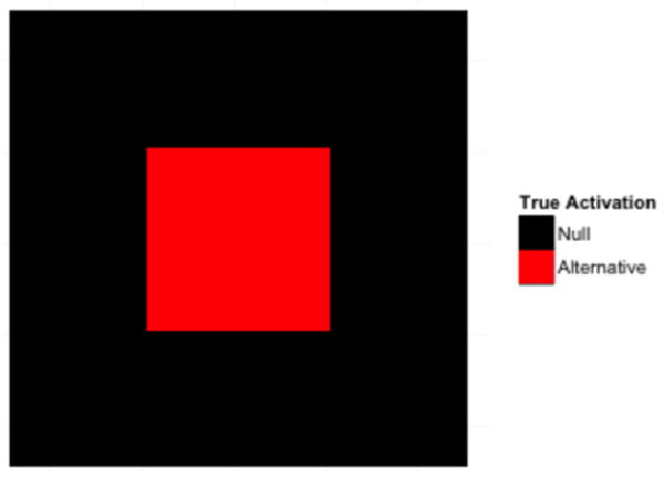
An overview of the underlying true signal found in the statistical maps used in the simulations. Each has dimensions 50×50. In the center of each map there is a square pattern of true activation with dimensions 20×20, shown in red.

In Fig. 4 we show examples of the effects of various approaches towards dealing with multiple comparisons. In the top row we show ten simulated t-maps. In the next row, we show the results analyzing these maps using an uncorrected threshold corresponding to α=0.10. The signal image of Fig. 3 is overlaid with white for voxels that exceed the threshold and are deemed active. Active voxels that fall inside of the red square are considered true positives, while those that fall outside the square are considered false positives. The false positive rate, false discovery rate, and power are listed under each image. As expected the false positive rate averages 10%. The third row shows the same images with the threshold designed to control the FWER at 0.10 using Bonferroni correction. Underneath each image, the number of false positives and reported power are listed. There is one false positive voxel in three of the 10 images (the third, sixth and eighth ones), at the cost of a significant increase in the number of false negatives. Finally, the bottom row shows similar results obtained using an FDR controlling procedure with q = 0.10, with false positive rate, false discovery rate, and power reported listed. The proportion of active voxels that are false positives is listed under each image, and as expected they average 0.10.

Figure 4.

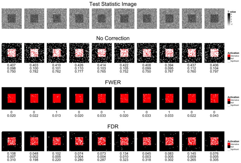
An overview of the effects of various approaches towards dealing with multiple comparisons. (Row 1) Ten t-maps were simulated. (Row 2) These maps were analyzed using an uncorrected threshold α= 0.10. Voxels that exceed the threshold and are considered active are indicated in white. Active voxels that fall inside of the red square shown in Fig. 3 are considered true positives, while those that fall outside the square are considered false positives. The false positive rate, false discovery rate, and power reported are listed under each image. The false positive rate averages 10% as expected. (Row 3) The same images with the threshold designed to control the FWER at 0.10 using Bonferroni correction. There is only one false positive in the 10 images, at the cost of a significant increase in the number of false negatives. The number of false positives and power reported is listed under each image (Row 4) Similar results obtained using an FDR controlling procedure using q=0.10. The false positive rate, false discovery rate, and power reported are listed under each image. The false discovery rate averages 10% as expected.

Fig. 5 illustrates the importance of signal-to-noise ratio (SNR) in the testing procedure. In the top row we show ten simulated t-maps that were simulated with constant signal, but at 10 different noise levels corresponding to SNR values ranging from 1 to 10. In this simulation, the true activation is again that depicted in Fig. 3. In the second, third and forth rows of Fig. 5 this signal image is overlaid with white where activation is detected. In the second row, we show the results of analyzing these maps using an uncorrected threshold corresponding to α=0.05. The third row shows the same images with the threshold designed to control the FWER at 0.05 using Bonferroni correction. Interestingly, for high SNR (right-hand side) the thresholded images are almost perfect, with all true activations detected and no false positives. The results are drastically worse for lower SNR (left-hand side) with an increasing number of false negatives. As these SNRs are more indicative of the levels seen in fMRI, this indicates potential problems with using this approach in the fMRI setting. Finally, the bottom row shows similar results obtained using an FDR controlling procedure with q=0.05. As the expected proportion of active voxels that are false positives is fixed in each image, both the number false positives and false negatives increase as the SNR increases.

Figure 5.

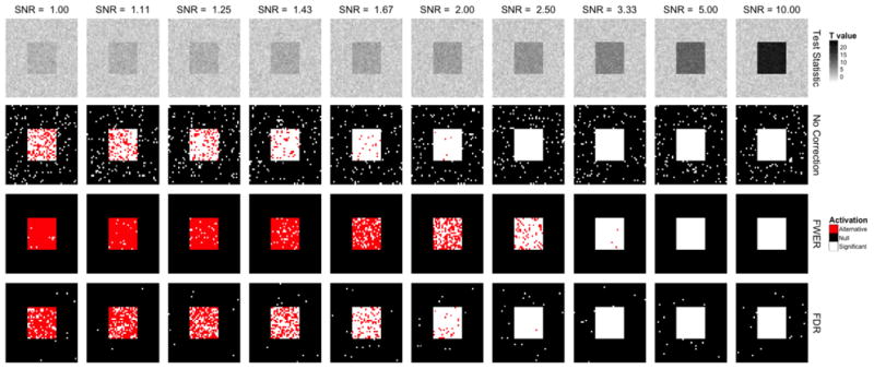
An overview of the effects of various approaches towards dealing with multiple comparisons at different signal-to-noise levels. (Row 1) Ten t-maps were simulated. (Row 2) These maps were analyzed using an uncorrected threshold corresponding α=0.05. Voxels that exceed the threshold and are considered active are indicated in white. Active voxels that fall inside of the red square shown in Fig. 3 are considered true positives, while those that fall outside the square are considered false positives. (Row 3) The same images with the threshold designed to control the FWER at 0.05 using Bonferroni correction. (Row 4) Similar results obtained using an FDR controlling procedure with q=0.05.

3.4. Cluster-extent Based Thresholding

In recent years perhaps the most common approach towards controlling for multiple comparisons in the neuroimaging community has been to use so-called cluster-extent based thresholding (10). Here statistically significant clusters are determined based on the number of contiguous voxels whose test statistic exceeds some pre-determined threshold. This is typically performed using a two-step procedure. First, a primary threshold, chosen in an ad hoc manner by the researcher, is used to threshold voxels according to their amplitude and determines clusters of supra-thresholded voxels. Second, a cluster-level extent threshold, expressed in terms of the number of contiguous voxels, is determined based on the distribution of cluster sizes under the null hypothesis of no activation in any of the voxels within the cluster.

Often the extent threshold is chosen in an arbitrary manner in the neuroimaging literature. This does not necessarily correct the problem of false positives, because imaging data are spatially smooth. Fig. 6 shows an example of an activation map with spatially correlated noise at three different smoothness levels. The top row shows the simulated t-statistic maps for each smoothness level, and the bottom row shows the result of analyzing these maps by thresholding at α = 0.1. Again, the signal map depicted in Fig. 3 is superimposed by white for voxels that exceed the threshold. Due to the inherent smoothness of the image, the false-positive activation regions (outside of the red square of true activation) tend to be contiguous regions consisting of multiple voxels, and would therefore in many situations survive cluster extent thresholds. Therefore, FWE- or FDR-corrected thresholds should be used whenever possible. Cluster-level extent thresholds that control the FWER can be determined by computing the sampling distribution of the size of the largest cluster of supra-thresholded voxels under the null hypothesis. This can be computed under the global null hypotheses of no signal using theoretical methods (e.g., Random Field Theory), Monte Carlo simulation, or nonparametric methods.

Figure 6.

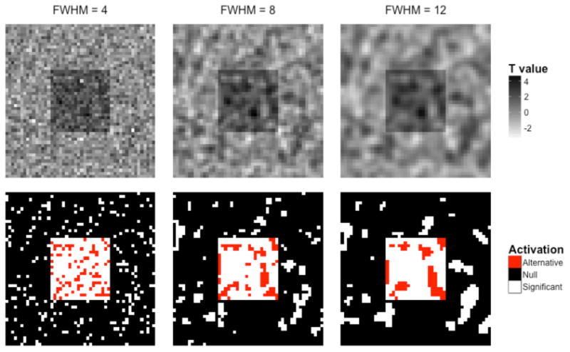
Imposing an arbitrary ‘extent threshold’ based on the number of contiguous activated voxels does not necessarily solve the problem of false positives. (Top) Using the same activation map as in the previous simulations, spatially correlated noise at three different levels of smoothness was added, and the corresponding t-maps were generated. (Bottom) These maps were thresholded at α=0.10. Due to the inherent smoothness of the image, the false-positives (outside of the squares) tend to be contiguous regions of multiple voxels that can easily be misinterpreted as regions of activity.

Cluster-extent based thresholding procedures take into consideration the possible dependencies between adjacent voxels. In addition, they tend to be more sensitive (i.e. have higher power) than other procedures that control the FWER. However, in contrast they also tend to have lower spatial specificity, particularly when clusters are large. The reason is that these procedures are not designed to determine the statistical significance of a specific voxel within the cluster, but instead describe the probability of obtaining a cluster of a given size or greater under the null hypothesis. Therefore they do not control the estimated false positive probability of each voxel in the region, but instead that of the region as a whole. This can be particularly problematic if a liberal primary threshold (e.g., p < 0.01) is used, as this will give rise to larger clusters and decrease the spatial specificity of any conclusions that can be made regarding the activations.

It has been argued (11) that the excessive use of liberal primary thresholds in the neuroimaging literature is problematic. They are most often used in underpowered studies, as they tend to give rise to significant clusters that are larger and appear more robust than can be obtained otherwise. However, large significant clusters tend to yield very little useful scientific information, particularly if they cross multiple anatomical boundaries. In addition, maps indicating regions that survive cluster extent thresholding are often erroneously interpreted as implying that all voxels and regions depicted are significant. However, in fact, if a single cluster covers two regions, it is unclear how the findings can be discussed in relation to either anatomical region in isolation.

4. Uncorrected Thresholds

Unfortunately, many published PET and fMRI studies do not actually make use of any multiple comparisons procedures. Instead they use arbitrary uncorrected thresholds with a ‘stringent’ threshold (e.g., p < .001). A likely reason is that with available sample sizes, corrected thresholds are so high that power to detect activations is extremely low. In fact, a published summary (4) of 11 whole-brain statistical maps showed that the average required p-value for whole-brain correction at p < 0.05 was p < 0.000072. This is substantially lower than the thresholds normally applied in the literature. This is extremely problematic when interpreting conclusions from individual studies, as many of the activated regions may simply be false positives. Hence, using stringent significance levels only goes so far in addressing the problem and ultimately makes subsequent replication studies substantially more important.

Because achieving sufficient power is often not possible in most neuroimaging studies, it does sometimes make sense to report results at an uncorrected threshold and use meta-analysis or a comparable replication strategy to identify consistent results across studies (12), with the caveat that uncorrected results from individual studies cannot be strongly interpreted by themselves. Ideally, a study would report both corrected results and results at a reasonable uncorrected threshold (e.g., p < .001 and 10 contiguous voxels) for archival purposes.

5. Alternative Approaches

Rather than performing hundreds of thousands of tests and correcting for multiple comparisons, many researchers are looking for alternatives. For example, instead of modeling and testing each parameter separately, it may ultimately be more appropriate to represent all the parameters of interest in a single model. In the imaging setting, one could imagine using a multi-level approach with voxels grouped within regions of interest. If properly constructed, this type of model could circumvent many of the issues discussed in this paper, at the cost of increased computational demands. For interested readers, the potential benefits of this type of approach are discussed in more detail in Lindquist and Gelman (13).

It is often argued that performing analysis in the Bayesian framework allows one to circumvent the multiple comparisons problem. While a Bayesian model that models all the parameters of interest simultaneously (as described above) would be a step in the right direction, simply fitting a voxel-wise multiple regression in a Bayesian framework does not necessary alleviate these concerns. Ultimately, the amount of protection provided by Bayesian methods depend strongly on the choice of prior distribution, and exactly quantifying the chance of obtaining false positives can be difficult in practice.

Instead of using more complicated models, another alternative is to use a more targeted approach towards testing. Many times the scientific question of interest dictates that a certain subset of the tests performed are of particular importance. For example, in the imaging setting we are often interested in focusing our analysis to certain pre-specified regions of interest. In this case one can focus entirely on voxels that lie within these regions. This can substantially reduce the burden of multiple comparison correction by limiting the number of voxels of interest. However, it is critical that the voxels to be tested be specified before actually viewing the data. Otherwise one risks ‘data dredging’ and uncovering biased results that will not be reproducible.

6. Effect Size Estimation

The study of individual differences and the estimation of brain-behavior correlations has become increasingly popular, as they are often taken as stronger evidence than activation alone that brain activity is related to some psychological processes of interest. However, these measures are susceptible to a number of issues, and this has led to substantial criticism of the manner in which they are often computed (14,15,16). One of the main problems is related to the difficulty of obtaining unbiased effect size estimates of the brain-behavior correlations in active regions of the brain. This is ultimately an issue intrinsically related to the multiple comparisons problem.

In neuroimaging research, the goal is often to first identify voxels that contain a particular effect and thereafter to estimate the size of the effect. The process of identifying voxels typically requires performing hypothesis tests at every voxel of the brain in order to detect the effect of interest, which presents a multiple testing problem that needs to be addressed. This problem has been the primary focus of the paper. However, as we will see below, the manner in which this is performed will also have a profound effect on the latter estimate of the effect size.

To illustrate, consider a hypothetical experiment consisting of 20 subjects. Suppose we perform an analysis that seeks to test whether there is significant correlation across subjects between a behavioral score and brain activity in every voxel of the brain. After computing the relevant test statistic in each voxel, we threshold the resulting statistical map and identify key regions of the brain related to the particular behavioral measure. Next we want to summarize the findings in a secondary analysis by computing summary statistics (e.g., the average correlation) for each active region.

If multiple comparisons correction is properly used, as discussed in the previous sections, identification of active voxels is not a problem. However, it is important to note that any effect-size estimates related to the manner in which voxels were chosen may be affected by selection bias. This is illustrated in Fig. 7, which shows the hypothetical distribution of the correlations across all voxels in the brain. This can reasonably be assumed to consist of a mixture of two distributions: one for non-active voxels whose correlations follow a normal distribution with mean 0, and another for active voxels whose correlations follow a Normal distribution with non-zero mean (0.6 in our example). Suppose that when testing for non-zero correlation, we deem any voxel whose correlation exceeds 0.7 as being significant. In our search for significant voxels, we have now conditioned them on having a large observed effect size. After all, voxels that survive the threshold must have a correlation of at least 0.7, and thus the average correlation for all active voxels in a given region will be well above that value and will be biased above the true mean correlation of 0.6.

Figure 7.

The hypothetical distribution of the correlation for all voxels in the brain is assumed to be a mixture of two distributions: one for non-active voxels whose correlations follow a Normal distribution with mean 0, and another for active voxels who follow a Normal distribution with mean 0.6. Suppose correlations exceeding 0.7 are deemed significant. Due to the manner in which voxels were selected, the average correlation for all active voxels will be substantially higher than the population average 0.6.

For these reasons, correlations reported in many fMRI studies are overstated because researchers tend to report only the highest correlations, or only those that exceed some threshold. This may lead to overestimation of the strength of the relationship between certain behavioral measures and specific brain patterns. Therefore, the practice of simply reporting the magnitude of the reported correlations is somewhat suspect. The fact that many imaging studies are underpowered adds an additional wrinkle, as estimates with relatively large standard errors are more likely to produce effect estimates that are larger in magnitude than estimates with relatively smaller standard errors, regardless of the true effect size.

To avoid bias it is critical that the statistic used to estimate the effect-size be independent of the criterion for selecting the voxels over which it is computed. Independence can be ensured by using independent data for selection (e.g. using part of the data to select voxels, and the other part to estimate the effect) or by using independent functional or anatomically defined ROIs. Alternatively, one can choose voxels based on whether their statistics show significant individual differences in the population (17), as this is a necessary condition for the underlying measure to be correlated with a behavioral measure. After all, if a given voxel shows the same value for all subjects it cannot be correlated with a behavioral measure that shows significant inter-subject variation. For this reason, one can pre-screen voxels to only focus on those that show a significant inter-subject variation. Hence, tests of inter-individual variance can be used to determine appropriate regions of interest and to test for brain-behavior correlations. This provides statistical maps of brain regions in which true inter-individual differences are large and reliable, without biasing voxel selection towards correlation with any particular behavioral measure, as the estimated variances are independent of the parameters used to compute the correlations.

7. Guidelines

When performing a large number of statistical tests, researchers should always use appropriate corrections for multiple comparisons that control either the FWER or the FDR. Either corrected or both corrected and uncorrected results should be reported and clearly labeled. In addition, it is important that the manner in which the correction was performed be made explicit in the article, as this will guide readers in interpreting the results. This can involve reporting the number of tests that were performed and, if possible, measures of the smoothness of the data to allow readers to assess the correlation between tests. In the neuroimaging context it should be made clear whether a voxel- or cluster-wise control was used. When cluster-wise control is used, both the primary threshold used to create the initial clusters and the cluster-extent threshold should be reported.

Whether to choose an FWER or FDR controlling procedure ultimately depends upon the scientific problem of interest. In different disciplines obtaining either a false positive or a false negative may be considered a more serious error. If the ‘cost’ of obtaining a single false positive is high, than FWER controlling procedures provide the best protection and should be used. If instead one were willing to accept a certain amount of false positives in order to guard against excessive false negatives, than FDR-controlling procedures would be more appropriate.

If there are strong a priori reasons to believe that a certain subset of tests are more likely to be significant, than it makes sense to focus on these tests to minimize the multiple comparisons problem. However, it is critical that these tests be determined before actually looking at the data and not as a result of a lack of significant findings among all tests after properly correcting for multiple comparisons. In this case one risks introducing false positives into the literature that cannot be reproduced in future studies.

Finally, as described in Section 6, the standard approach of estimating effect sizes for voxels that survive a multiple comparisons threshold tends to overestimate the true effect size. In certain situations (e.g., when the effect size is large and/or the variance is small), this bias may be small and the estimate can still provide useful information. However, this is often not the case, and readers may inflate the importance or meaning of the reported estimates without understanding the selection issue. Therefore it is critical that when reporting an effect size that appropriate guidelines for interpreting the value are provided.

8. Conclusions

The multiple comparisons problem arises when a family of statistical tests is simultaneously performed. In many modern high-dimensional scientific endeavors, such as genomics and imaging, the multiple comparisons problem is more prevalent and consequential than ever. Failure to properly account for multiple comparisons will ultimately lead to heightened risks for false positives and erroneous conclusions.

Although we have focused our attention on neuroimaging in this paper, the problem is certainly not unique to this field. Any time that multiple tests are performed without proper correction, there is the potential to seriously impact the resulting conclusions. The good news is that there exist a number of established techniques that can be used to correct for multiple comparisons. When properly applied, these methods provide adequate control over false positives.

Most of these methods are concerned with either controlling the family-wise error rate or the false discovery rate, and in this paper we have discussed a variety of methods for controlling both. Each of these methods provides a principled guide for choosing a higher significance threshold compared to what is used for individual tests, as a means of compensating for the large number of tests being performed. If the chosen threshold is too conservative, we risk losing the power to detect meaningful results. If instead the threshold is too liberal, this will result in an excessive number of false positives. Ideally, we want a threshold that maximizes the number of true positives while minimizing the risk of false positives. The methods discussed in this paper are all concerned with choosing this threshold in a principled manner.

Whether one chooses to control the FWER or the FDR ultimately depends on the situation or simply personal preference. What is crucial is that some sort of principled correction for multiple comparisons be made and discussed in detail in the methods sections of papers, which will allow readers to properly evaluate subsequent results and claims in an appropriate manner.

References

- 1.Button KS, Ioannidis JP, Mokrysz C, Nosek BA, Flint J, Robinson ES, Munafò MR. Power failure: why small sample size undermines the reliability of neuroscience. Nature Reviews Neuroscience. 2013;14(5):365–376. doi: 10.1038/nrn3475. [DOI] [PubMed] [Google Scholar]
- 2.Ioannidis JP. Why most published research findings are false. PLoS medicine. 2005;2(8):e124. doi: 10.1371/journal.pmed.0020124. [DOI] [PMC free article] [PubMed] [Google Scholar]
- 3.Storey JD, Tibshirani R. Statistical significance for genomewide studies. Proceedings of the National Academy of Sciences. 2003;100(16):9440–9445. doi: 10.1073/pnas.1530509100. [DOI] [PMC free article] [PubMed] [Google Scholar]
- 4.Nichols T, Hayasaka S. Controlling the familywise error rate in functional neuroimaging: a comparative review. Statistical methods in medical research. 2003;12(5):419–446. doi: 10.1191/0962280203sm341ra. [DOI] [PubMed] [Google Scholar]
- 5.Genovese CR, Lazar NA, Nichols T. Thresholding of statistical maps in functional neuroimaging using the false discovery rate. Neuroimage. 2002;15(4):870–878. doi: 10.1006/nimg.2001.1037. [DOI] [PubMed] [Google Scholar]
- 6.Wager T, Hernandez L, Jonides J, Lindquist M. Elements of Functional Neuroimaging. Handbook of psychophysiology. 2007:19. [Google Scholar]
- 7.Lindquist MA. The statistical analysis of fMRI data. Statistical Science. 2008;23(4):439–464. [Google Scholar]
- 8.Worsley KJ, Taylor JE, Tomaiuolo F, Lerch J. Unified univariate and multivariate random field theory. Neuroimage. 2004;23:S189–S195. doi: 10.1016/j.neuroimage.2004.07.026. [DOI] [PubMed] [Google Scholar]
- 9.Benjamini Y, Hochberg Y. Controlling the false discovery rate: a practical and powerful approach to multiple testing. Journal of the Royal Statistical Society. Series B (Methodological) 1995:289–300. [Google Scholar]
- 10.Poline JB, Mazoyer BM. Analysis of individual positron emission tomography activation maps by detection of high signal-to-noise-ratio pixel clusters. Journal of Cerebral Blood Flow & Metabolism. 1993;13(3):425–437. doi: 10.1038/jcbfm.1993.57. [DOI] [PubMed] [Google Scholar]
- 11.Woo CW, Krishnan A, Wager TD. Cluster-extent based thresholding in fMRI analyses: Pitfalls and recommendations. NeuroImage. 2014;91:412–419. doi: 10.1016/j.neuroimage.2013.12.058. [DOI] [PMC free article] [PubMed] [Google Scholar]
- 12.Wager TD, Lindquist M, Kaplan L. Meta-analysis of functional neuroimaging data: current and future directions. Social cognitive and affective neuroscience. 2007;2(2):150–158. doi: 10.1093/scan/nsm015. [DOI] [PMC free article] [PubMed] [Google Scholar]
- 13.Lindquist MA, Gelman A. Correlations and Multiple Comparisons in Functional Imaging: A Statistical Perspective (Commentary on Vul et al., 2009) Perspectives on Psychological Science. 2009;4:310–313. doi: 10.1111/j.1745-6924.2009.01130.x. [DOI] [PubMed] [Google Scholar]
- 14.Vul E, Harris C, Winkielman P, Pashler H. Puzzlingly high correlations in fMRI studies of emotion, personality, and social cognition. Perspectives on psychological science. 2009;4(3):274–290. doi: 10.1111/j.1745-6924.2009.01125.x. [DOI] [PubMed] [Google Scholar]
- 15.Kriegeskorte N, Simmons WK, Bellgowan PS, Baker CI. Circular analysis in systems neuroscience: the dangers of double dipping. Nature neuroscience. 2009;12(5):535–540. doi: 10.1038/nn.2303. [DOI] [PMC free article] [PubMed] [Google Scholar]
- 16.Kriegeskorte N, Lindquist MA, Nichols TE, Poldrack RA, Vul E. Everything you never wanted to know about circular analysis, but were afraid to ask. Journal of Cerebral Blood Flow & Metabolism. 2010;30(9):1551–1557. doi: 10.1038/jcbfm.2010.86. [DOI] [PMC free article] [PubMed] [Google Scholar]
- 17.Lindquist MA, Spicer J, Asllani I, Wager TD. Estimating and testing variance components in a multi-level GLM. NeuroImage. 2012;59(1):490–501. doi: 10.1016/j.neuroimage.2011.07.077. [DOI] [PMC free article] [PubMed] [Google Scholar]