

SUMMARY
The number of effectively independent tests performed in genome-wide association studies and the corresponding genome-wide significance level varies by population. Therefore, a common p-value threshold may be inappropriate. To assess this, we estimated the number of independent SNPs for all Phase 3 HapMap samples using the LD pruning function in PLINK. We also used an autocorrelation-based approach to verify the HapMap findings, and tested it on 1000 Genomes data to estimate the number of independent tests in whole genome sequences. The number of effectively independent tests performed in genome-wide association studies (GWAS) varies by population, making a universal p-value threshold inappropriate. We estimated the number of independent SNPs in Phase 3 HapMap samples by: (1) the LD pruning function in PLINK, and (2) an autocorrelation-based approach. Autocorrelation was also used to estimate the number of independent SNPs in whole genome sequences from 1000 Genomes. Both approaches yielded consistent estimates of numbers of independent SNPs, which were used to calculate new population-specific thresholds for genome-wide significance. African populations had the most stringent thresholds (1.49×10⁻⁷ for YRI at r2=0.3), East Asian populations the least (3.75×10⁻⁷ for JPT at r2=0.3). We also assessed how using population-specific significance thresholds compared to using a single multiple testing threshold at the conventional 5×10⁻⁸ cutoff. Applied to a previously published GWAS of melanoma in Caucasians, our approach identified two additional genes, both previously associated with the phenotype. In a Chinese breast cancer GWAS, our approach identified 48 additional genes, 19 of which were in or near genes previously associated with the phenotype. We conclude that the conventional genome-wide significance threshold generates an excess of Type 2 errors, particularly in GWAS performed on more recently founded populations.
Keywords: genome-wide threshold, GWAS, HapMap, linkage disequilibrium, autocorrelation
INTRODUCTION
Linkage analyses and association studies are the two most popular methods used to identify risk alleles for human disease. Linkage analyses have been most successful for monogenic, Mendelian disorders because the causal alleles have large effect sizes and are more common in multiplex pedigrees. For more common diseases, such as diabetes, schizophrenia, and most cancers, in which the connections between genotype and phenotype are usually subtle and complex, association studies provide greater statistical power (Risch and Merikangas, 1996).
Recent advances in genotyping and sequencing technology have made “agnostic” high-throughput association study designs, in which many interrogated loci are chosen using statistical rather than biological criteria, the predominant approach for the identification of genes that predispose to disease. Genome-wide association studies (GWAS) and high-throughput, massively parallel sequencing permit investigators to interrogate millions of single nucleotide polymorphisms (SNPs) throughout the genome in a single study. However, performing such a large number of statistical tests is expected to generate an abundance of false positive findings, or type 1 errors, if the threshold for significance is not appropriately strict. The number of false positive results typically has been managed by controlling the family-wise error rate (FWER), namely, the probability of at least one false discovery within a family of hypotheses. A conservative approach to assure that the FWER is below a set threshold (α) in a given GWAS is to apply a Šidák (1) or a Bonferroni (2) correction,
P(study-wide type I error) = 1 − (1 − α)1/n
P(study-wide type I error) = α/n
where n is the number of independent tests (Šidák, 1967). The Bonferroni correction, a close approximation of the more rigorous Šidák correction, has been used when approximating the standard for GWAS significance, with p < 5x10⁻⁸ corresponding to an α of 0.05 for one million independent tests (Altshuler et al., 2008). This correction for genetic analyses was recommended after simulated data were used to estimate the number of independent variants in the human genome, based on patterns of linkage disequilibrium (LD) primarily based on European-ancestry individuals (Pe’er et al., 2008). Although this study provided an initial estimate of the number of independent tests and a corresponding threshold for significance, there is now an opportunity to refine this threshold using densely genotyped reference populations and data from high-throughput genetic studies of traits.
We argue that a more accurate and population-specific empirical estimate of the number of independent tests necessary to control the FWER can now be used. Since the 5×10⁻⁸ threshold was estimated in individuals of European ancestry, it is a crude proxy for the genomic landscape in other populations because LD and allele frequencies vary with ancestry. Consequently, the significance threshold required to control the FWER does not correspond to the number of tests performed in any real study and also varies with ancestry. Therefore, although this canonical threshold will effectively limit type 1 error, it almost certainly inflates false negative findings, or type 2 errors (Williams and Haines, 2011), and is not tuned to the data at hand or diverse populations with distinct demographic histories in general. An imbalance of error rates permitting an excess of type 2 error may be more problematic in the long term because type 1 errors are more easily identified in subsequent studies, and the resources necessary to perform very large GWAS to overcome the bias toward type 2 errors are finite (Williams and Haines, 2011).
Less conservative methods have been suggested to limit the inflation of type 2 error in high density genetic analyses. The False Discovery Rate (FDR) controls the expected proportion of false positives among the rejected null hypotheses and is a popular, less conservative alternative to Bonferroni correction (Benjamini Y, 1995). However, FDR also assumes independence of hypotheses; therefore, if many SNPs in strong LD are present on an array, it can suffer from a loss of statistical power. Other methods such as permutation procedures can provide an accurate FWER, but implementation is computationally challenging and not feasible in consortium studies. Furthermore, the results of permutation testing are difficult to extrapolate beyond the data set from which they are generated (Hoggart et al., 2008).
Several studies have proposed to correct only for the effective number of independent tests performed, Meff, a number that has been estimated by using principal components or the analysis of the LD structure in the genome (Cheverud, 2001, International HapMap, 2005, Gao X, 2008, Duggal et al., 2008). LD structure has been previously analyzed using a Solid Spine of LD measure, the 4-Gamete Rule, and the Gabriel and Nyholt methods (Duggal et al., 2008, Nyholt, 2004, Hudson and Kaplan, 1985, Gabriel et al., 2002, Barrett et al., 2005). While some of these methods improve type 2 error rates and perform similarly to the Bonferroni correction in high and moderate LD settings, it has been suggested that the use of the traditional r2 measure might improve the Meff estimation even further (Nicodemus et al., 2005). Moreover, perhaps because of the requirement of additional software and analytics necessary to estimate Meff, these approaches have not been widely adopted. Hence, the genome-wide threshold of 5×10⁻⁸ continues to be the convention.
We propose a much simpler and more practical solution: empirically estimating Meff using the r2-based LD pruning option in PLINK, the software most commonly used for GWAS analyses. This approach adjusts for a more natural number of independent tests, likely reducing the type 2 error rate by uncovering more true associations and thus accounting for more heritability without dramatically increasing sample size, sample utilization, and study cost. We further validate this approach with an alternative autocorrelation method.
Variable LD patterns have been well documented among the CEU, YRI, CHB, and JPT samples used in Phase 1 of the HapMap project (International HapMap, 2005, International HapMap, 2003). Because the correlational structures of SNPs are specific to populations, the degree of overcorrection using the canonical genome-wide threshold also varies. Phase 3 of the International HapMap Project provides estimates of LD structure in additional samples from several more major populations and admixed groups: ASW, CHD, GIH, LWK, MXL, MKK, and TSI. Here, we present methods to calculate correlation-based Meff values, providing genome-wide thresholds that correspond to the Phase 3 HapMap samples. We demonstrate that the extent of the overcorrection from a Bonferroni-based genome-wide threshold is proportional to the founding date of a given population or its distance from Africa. We then use the LD pruning-based method to establish study-specific thresholds in two genome-wide association studies: a cutaneous melanoma study in non-Hispanic whites and a breast cancer study in East Asians. We then re-evaluate the significant associations at the various Meffs defined by new LD thresholds for each GWAS and show that substantial type 2 error occurred when the conservative 5×10⁻⁸ standard of significance was used.
There is no generally agreed upon r2 threshold below which SNPs are classified as independent. To avoid an arbitrary choice of r2 in our LD-based method, we complemented the PLINK-based approach with autocorrelation to estimate the number of independent tests performed in a given association study. The estimation of Meff was addressed empirically by assessing the autocorrelation of genotype one individual at a time. Autocorrelation of genotype can be viewed as linkage disequilibrium at the limit of one individual. While it is not feasible to estimate linkage disequilibrium without partitioning a chromosome into multiple disjoint blocks or sliding windows (Cheverud, 2001, Nyholt, 2004, Li and Ji, 2005, Moskvina and Schmidt, 2008, Han et al., 2009, Ramos et al., 2011), it is computationally efficient to estimate autocorrelation for one individual over an entire chromosome. This approach is independent of (simulated or measured) phenotypes, and does not require p-values, thereby decoupling the effective number of markers from the testing burden for any particular type of statistical test of association, any assumption of the asymptotic distribution of test statistics, or any p-value threshold. Using data from each GWAS, the HapMap samples as well as whole genome sequences (Genomes Project et al., 2012), we show that the intra-population patterns of Meff estimates we obtained with LD pruning are highly consistent with this robust approach.
MATERIALS AND METHODS
HapMap thresholds determined by PLINK pruning
To study the effects of population-specific LD structure on genome-wide significance thresholds, we examined genotype data (Affymetrix® Genome-Wide Human SNP Array 6.0, Illumina Human 1M-single BeadChip) from the second release of the International HapMap Project Phase 3. Our analysis was restricted to the founders in each of the 11 samples, reducing the sample size from 1,184 individuals in the original data set to 988 (Table S1). We excluded SNPs with minor allele frequencies below 0.05, as LD among rare alleles is often weak and power to detect associations is low, and genotyping call rates less than 95%. We excluded individuals for whom more than 5% of SNPs available on the platform could not be called. The number of markers passing quality controls for each sample is shown in Table S1. The data were subsequently pruned for linkage disequilibrium in PLINK (Purcell et al., 2007, Purcell), using a 100 SNP window size, a 5 SNP window shift, and r2 ranging from 0.1 to 1.0 in increments of 0.1. The number of SNPs remaining after this pruning process was considered to be equal to the number of effectively independent SNPs for each population and each r2 threshold. Population-specific genome-wide significance thresholds were then determined with the Bonferroni method (2), dividing an alpha of 0.05 by the number of effectively independent SNPs as determined by the PLINK pruning, over a range of r2 values (i.e., 0.05/(number of effectively independent SNPs)).
Cutaneous Melanoma GWAS thresholds
We calculated genome-wide significance thresholds using the same LD pruning technique for a cutaneous melanoma GWAS data set. The study included 2,830 non-Hispanic white patients seen at MD Anderson, as previously described (Amos et al., 2011). The same SNP and individual quality control criteria were used as for the HapMap data (Table S2). The GWAS data were pruned for LD as described above. The Bonferroni correction (2) was used to establish genome-wide significance, dividing an alpha of 0.05 by the number of effectively independent SNPs as determined by PLINK. The resulting thresholds derived from the study sample’s genotype data were compared to those calculated for the HapMap CEU sample. The SNPs interrogated in the GWAS were reevaluated using the different thresholds established by the various r2 cutoffs. SNPs falling between the population-specific thresholds and 5×10⁻⁸ were assigned to genes using the SNP Functional Prediction tool in SNPinfo (Xu and Taylor, 2009). The criterion for previous association of these genes with cutaneous melanoma was at least one statistically significant finding in the literature. To better understand the correlational structure of associating SNPs, we examined pairwise correlations of all SNPs from the same chromosome that remained significant after a multiple testing correction (for r2 = 0.1). This provides a summary of the correlation structure of all SNPs nominally associated with disease.
Shanghai Breast Cancer Study GWAS thresholds
We evaluated associations at various population-specific genome-wide thresholds for the Shanghai Breast Cancer Study and the Shanghai Breast Cancer Survival Study GWAS, a cohort of 5,161 East Asian females aged 20 to 75 with stage I to stage IV disease. The details of the studies and the sample have been described elsewhere (Shu et al., 2009, Shu et al., 2012). We applied the same quality control criteria and LD pruning method as above to the Shanghai sample. Putatively associating SNPs were assessed using literature searches. If the SNPs falling between the population-specific thresholds and 5×10⁻⁸ were in genes with previous evidence of association, or evidence published subsequently in larger studies, we considered them type 2 error resulting from the usage of an overly conservative genome-wide threshold.
Estimating Meff using Autocorrelation
We also performed a second, independent analysis to determine the effective number of independent tests. Specifically, autocorrelation was performed on Phase 3 HapMap samples and each GWAS study, using the same inclusion criteria as above, and separately on whole genome sequence data. Sequence data were retrieved from the 1000 Genomes phase 1 version 3 release (ftp://ftp-trace.ncbi.nih.gov/1000genomes/ftp/release/20110521/). All SNPs were extracted for the autosomal and X chromosomes. The effective numbers of markers were estimated by autocorrelation. Briefly, genotypes were recoded as 0, 1, or 2 copies of the minor allele, corresponding to an additive genetic model. For each chromosome for each individual, we fit an autoregressive model. The notation for an autoregressive model of order p is AR(p) and the model is defined as , in which c is a constant, φ1,…,φp are the parameters, and εt is white noise. The order of the fitted autoregressive model is chosen by minimizing the Akaike information criterion (Plummer, 2012). For the best fit model, the effective number of markers is estimated by first dividing the residual variance by (1 minus the sum of the autoregression coefficients)2, and then multiplying the number of markers by the variance of the recoded genotypes and dividing by the former quotient. For each chromosome, the maximum value of the order is the largest integer smaller than 10×log10 (number of markers). If this default value is too small, then the effective number of markers may be overestimated, leading to overly conservative significance levels and loss of power. Finally, the effective numbers of markers were summed by chromosome and averaged across individuals for each sample. All calculations were performed using R, including the effective Size function from the R library coda (Plummer, 2012, R Core Team, 2013). Note that there is no pruning in this approach.
RESULTS
Population-Specific Genome-wide Thresholds Using the LD-pruning Method
In the HapMap data, the numbers of SNPs were population-specific in both the pre-LD-pruned and post-LD-pruned data. Samples of African ancestry (LWK, MKK, YRI, and the admixed ASW) had the highest number of independent SNPs remaining throughout the range of r2 values used for LD pruning (e.g., 825,819 – 867,326 at r2 = 0.8, Table 1). The East Asian samples (CHB, CHD, and JPT) had the fewest number of independent SNPs (402,860 – 414,300 at r2 = 0.8), and those of European and Indian origin (CEU, TSI, GIH, and the admixed MXL) were intermediate (489,663 – 516,945 at r2 = 0.8, Table 1).
Table 1. SNPs remaining after LD pruning in HapMap samples.
Number of independent SNPs remaining per Phase 3 HapMap sample after pairwise filtering at various r2 thresholds (the largest and smallest numbers for each LD cutoff are in bold and italics, respectively).
| r2 | LWK | MKK | YRI | GIH | TSI | CEU | CHB | CHD | JPT | ASW | MXL |
|---|---|---|---|---|---|---|---|---|---|---|---|
| 1 | 1,328,749 | 1,337,073 | 1,309,097 | 1,235,674 | 1,235,949 | 1,219,753 | 1,119,904 | 1,106,284 | 1,117,554 | 1,393,867 | 1,196,368 |
| 0.9 | 974,647 | 967,348 | 935,766 | 633,672 | 620,658 | 602,645 | 521,707 | 521,346 | 503,177 | 995,636 | 652,180 |
| 0.8 | 856,602 | 840,862 | 825,819 | 516,040 | 502,103 | 489,663 | 414,300 | 412,618 | 402,860 | 867,326 | 516,945 |
| 0.7 | 755,927 | 735,833 | 728,240 | 430,845 | 418,002 | 407,158 | 342,172 | 339,829 | 333,235 | 761,504 | 427,405 |
| 0.6 | 659,587 | 638,159 | 634,341 | 358,906 | 347,091 | 337,846 | 283,669 | 281,764 | 276,288 | 657,335 | 351,380 |
| 0.5 | 562,489 | 542,126 | 539,933 | 293,712 | 282,876 | 275,122 | 231,656 | 230,143 | 225,494 | 552,343 | 283,864 |
| 0.4 | 462,019 | 443,578 | 441,146 | 231,949 | 222,932 | 216,572 | 183,781 | 183,183 | 178,407 | 443,185 | 220,178 |
| 0.3 | 351,547 | 339,195 | 335,907 | 171,559 | 165,035 | 160,406 | 137,853 | 137,402 | 133,477 | 323,674 | 157,020 |
| 0.2 | 226,994 | 225,685 | 220,441 | 112,295 | 108,185 | 105,470 | 92,952 | 92,685 | 89,085 | 188,830 | 93,732 |
| 0.1 | 87,815 | 98,223 | 94,146 | 52,004 | 51,508 | 51,135 | 47,141 | 47,295 | 44,298 | 62,489 | 36,164 |
The numbers of SNPs remaining after LD pruning were used to calculate population-specific genome-wide significance thresholds, using a Bonferroni multiple testing adjustment (2). With an r2 level of 0.8 as the cutoff for establishing the number of independent tests, the estimated significance threshold was 6.05×10⁻⁸ for YRI, 1.02×10⁻⁷ for CEU, and 1.24×10⁻⁷ for JPT (Figures 1, S1; Table S3). When the number of SNPs with r2 < 0.5 was used to estimate the number of independent tests, the significance threshold was 9.26×10⁻⁸ for YRI, 1.82×10⁻⁷ for CEU, and 2.22×10⁻⁷ for JPT. When r2 < 0.1 was used, the estimated significance threshold was 5.31×10⁻⁷ for YRI, 9.78×10⁻⁷ for CEU, and 1.13×10⁻⁶ for JPT. As expected, the three African samples along with the admixed ASW sample had similar thresholds when r2 varied between 0.3 and 0.9. At LD pruning r2 of 0.2 and 0.1, the admixed ASW sample had stronger LD than the other African samples, thereby defining fewer independent SNPs and a more easily reached significance threshold. GIH, CEU, TSI, and MXL had similar thresholds in the 0.3 – 0.9 r2 range, but MXL had more independent SNPs in LD at r2 levels of 0.1 and 0.2. The CHB, CHD, and JPT samples had similar significance thresholds across the entire r2 range (Table S3).
Figure 1. Significance threshold change by linkage disequilibrium in Phase 1 HapMap samples.
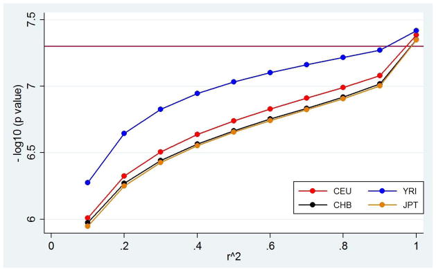
Comparison of the conventional genome-wide threshold (maroon) to the population-specific genome-wide threshold calculated by LD pruning the HapMap CHB sample (black), JPT sample (orange), CEU sample (red) and YRI sample (blue).
Re-evaluating SNPs in a Cutaneous Melanoma GWAS in a Caucasian Sample
In addition to using existing databases, we also applied LD pruning to actual GWAS data to assess whether our results from the HapMap data matter in practice. The genome-wide significance thresholds in the non-Hispanic white melanoma study compared favorably with those for the CEU sample from Phase 3 of HapMap, diverging only at very high LD levels (Figure 2A; Table 2). The actual GWAS data set had fewer SNPs interrogated (736,303 SNPs) than the CEU HapMap sample (1,219,753 SNPs); therefore, as expected, there were fewer independent tests remaining at higher r2 cutoffs (Tables 1, 2). For example, pruning at r2 = 0.9, the genome-wide significance threshold for the actual GWAS data was 9.82×10⁻⁸ compared to 8.30×10⁻⁸ from the CEU HapMap data. However, when the LD pruning cutoffs were lowered, the two data sets produced similar thresholds, consistent with a high level of SNP redundancy in both the HapMap and GWAS data. When LD pruning was carried out at an r2 of 0.5, the threshold from the melanoma GWAS became 1.91×10⁻⁷ compared to 1.82×10⁻⁷ for CEU, while at an r2 of 0.1 it was 8.80×10⁻⁷ for the GWAS versus 9.78×10⁻⁷ for CEU.
Figure 2. Significance threshold variation change by linkage disequilibrium in GWAS data and corresponding HapMap proxies.


A) Changes in p-value thresholds as derived from a GWAS for melanoma in non-Hispanic whites and from the HapMap CEU samples. Comparison of the conventional genome-wide significance threshold (gold) with the population-specific genome-wide threshold calculated by applying autocorrelation to the cutaneous melanoma GWAS data (blue), population specific genome-wide thresholds calculated by LD pruning the Phase 3 HapMap CEU sample (black) and population specific genome-wide thresholds calculated by LD pruning the cutaneous melanoma GWAS data (red).
B) Changes in p-value thresholds as derived from a GWAS for breast cancer in an East Asian sample and the HapMap CHB sample. Comparison of the conventional genome-wide significance threshold (gold) with the population-specific genome-wide threshold calculated by applying autocorrelation to Shanghai Breast Cancer Study GWAS data (blue), population specific genome-wide thresholds calculated by LD pruning the Phase 3 HapMap CHB sample (black) and population specific genome-wide thresholds calculated by LD pruning the Shanghai Breast Cancer Study GWAS data (red).
Table 2. SNPs remaining after LD-pruning and corresponding thresholds in melanoma and breast cancer GWAS.
Number of independent tests and multiple testing adjusted p-value thresholds for the cutaneous melanoma GWAS in a non-Hispanic Caucasian sample and a breast cancer GWAS in an East Asian sample, at various LD pruning r2 levels and by autocorrelation.
| r2 | Melanoma GWAS indep. tests | Melanoma GWAS p-value thershold | Breast Cancer GWAS indep. tests | Breast Cancer GWAS p-value threshold |
|---|---|---|---|---|
| 1 | 736,303 | 6.79×10⁻⁸ | 584,593 | 8.55×10⁻⁸ |
| 0.9 | 509,102 | 9.82×10⁻⁸ | 347,523 | 1.44×10⁻⁷ |
| 0.8 | 442,520 | 1.13×10⁻⁷ | 286,368 | 1.75×10⁻⁷ |
| 0.7 | 379,219 | 1.32×10⁻⁷ | 244,848 | 2.04×10⁻⁷ |
| 0.6 | 318,629 | 1.57×10⁻⁷ | 209,557 | 2.39×10⁻⁷ |
| 0.5 | 262,280 | 1.91×10⁻⁷ | 177,619 | 2.82×10⁻⁷ |
| 0.4 | 208,672 | 2.40×10⁻⁷ | 146,712 | 3.41×10⁻⁷ |
| 0.3 | 157,074 | 3.18×10⁻⁷ | 115,681 | 4.32×10⁻⁷ |
| 0.2 | 106,645 | 4.69×10⁻⁷ | 83,491 | 5.99×10⁻⁷ |
| 0.1 | 56,880 | 8.80×10⁻⁷ | 49,523 | 1.01×10⁻⁶ |
| Autocorrelation | 137,069 | 3.64x10⁻⁷ | 91,099 | 5.49x10⁻⁷ |
SNPs not meeting the 5×10⁻⁸ threshold in the melanoma study were then reevaluated using the genome-wide significance thresholds obtained by LD pruning the GWAS data (Table 3). Seven additional SNPs were found between the p-values 5×10⁻⁸ and 8.80×10⁻⁷, the threshold for LD pruning at r2 of 0.1. All seven SNPs were in genes previously associated with cutaneous melanoma (Barrett et al., 2011, Falchi et al., 2009, Bishop et al., 2009, Stefanaki et al., 2013). Four of the SNPs were in or near the MTAP gene on chromosome 9, while the remaining three were in DEF8, AFG3L1, and DBNDD1 on chromosome 16. Other SNPs in DEF8 and AFG3L1 were identified using the conventional p-value cutoff, but no SNPs in DBNDD1 were. The DBNDD1 SNP, rs10852628, can be found at an LD pruning r2 of 0.9, while all MTAP SNPs require an r2 of 0.1. rs10852628 is correlated with SNPs mapping to other genes on chromosome 16, and it might be tagging the same causal variant as the other SNPs (Figure S2). The SNPs in and around MTAP are the only ones with p-values below 8.80×10⁻⁷ that are located on chromosome 9.
Table 3. Most significant SNPs in the melanoma GWAS.
Single Nucleotide Polymorphisms from the cutaneous melanoma GWAS with p-values less than 1×10⁻⁶.
| Chr. | SNP | Gene | OR | 95% CI | p-value |
|---|---|---|---|---|---|
| 16 | rs4785751 | DEF8 | 0.7 | 0.62–0.78 | 1.13×10⁻¹⁰ |
| 16 | rs4408545 | AFG3L1 | 0.7 | 0.63–0.78 | 4.43×10⁻¹⁰ |
| 16 | rs11076650 | AFG3L1 | 1.4 | 1.25–1.56 | 2.02×10⁻⁹ |
| 16 | rs8051733 | DEF8 | 1.41 | 1.26–1.58 | 3.80×10⁻⁹ |
| 16 | rs7195043 | DEF8 | 0.72 | 0.64–0.80 | 5.18×10⁻⁹ |
| 16 | rs11648898 | AFG3L1 | 1.53 | 1.32–1.77 | 1.62×10⁻⁸ |
| 15 | rs1129038 | HERC2 | 0.69 | 0.61–0.79 | 2.58×10⁻⁸ |
| 15 | rs12913832 | HERC2 | 0.69 | 0.61–0.79 | 4.31×10⁻⁸ |
| 16 | rs4785759 | AFG3L1 | 1.36 | 1.22–1.52 | 4.42×10⁻⁸ |
| 16 | rs4785752 | DEF8 | 1.35 | 1.21–1.51 | 5.66×10⁻⁸ |
| 16 | rs10852628 | DBNDD1 | 1.39 | 1.23–1.57 | 6.96×10⁻⁸ |
| 9 | rs7033503 | MTAP | 0.76 | 0.68–0.84 | 5.50×10⁻⁷ |
| 16 | rs4238833 | AFG3L1 | 1.33 | 1.19–1.49 | 5.78×10⁻⁷ |
| 9 | rs7848524 | MTAP | 1.32 | 1.18–1.47 | 6.84×10⁻⁷ |
| 9 | rs6475552 | MTAP | 1.31 | 1.18–1.46 | 8.41×10⁻⁷ |
| 9 | rs2383202 | MTAP | 1.31 | 1.18–1.46 | 8.70×10⁻⁷ |
| 9 | rs12380505 | MTAP | 1.31 | 1.78–1.46 | 9.41×10⁻⁷ |
| 16 | rs258322 | CDK10 | 1.55 | 1.30–1.84 | 9.63×10⁻⁷ |
Bold and italicized – SNPs missed by using the 5×10⁻⁸ genome-wide significance threshold
Re-evaluating SNPs in a Breast Cancer GWAS in an East Asian Sample
LD pruning of the Shanghai data at various r2 levels produced a pattern of population-specific genome-wide significance thresholds similar to that obtained using the CHB and other East Asian samples from Phase 3 of HapMap (Figure 2B). Because the Shanghai GWAS data had fewer SNPs interrogated (584,593 SNPs) than the CHB HapMap data (1,119,904 SNPs), there were fewer independent tests remaining at high r2 levels used for pruning (Tables 1, 2). The population-specific genome-wide significance thresholds for the breast cancer GWAS data ranged from 8.55x10⁻⁸ (no LD pruning) to 1.01×10⁻⁶ (corresponding to r2 = 0.1, Table 2).
Ninety SNPs associated with breast cancer in the Shanghai study at a p-value between 5×10⁻⁸ and the population-specific threshold of 1.01×10⁻⁶. Of these SNPs, 21 were in genes already identified as significant at p< 5×10⁻⁸ in this dataset. Of the remaining 69 SNPs, 28 (41%) mapped to genes previously associated with breast cancer. More specifically, 58 SNPs were in 48 different genes (10 SNPs in ESR1, 2 SNPs in ZBTB20, and 46 SNPs in 46 other genes) of which 19 (40%) had support for association with breast cancer in the literature (Table S4). At an LD-pruning level of r2 = 0.5, corresponding to a p-value threshold of 2.82×10⁻⁷, 32 new SNPs achieved population-specific significance, 13 of which (41%) mapped to genes previously associated with the phenotype. Of these 32 SNPs, seven were intergenic and 25 mapped to 21 different genes; nine of the 21 genes (43%) have been previously associated with breast cancer (Table S4). Even at the more conservative LD pruning level of r2 = 0.8, 21 new SNPs achieved population-specific significance, eight of which (38%) were in genes previously associated with the phenotype. Of the 21 SNPs, six were intergenic and 15 mapped to 13 genes; six of the 13 genes (46%) have been previously associated with breast cancer (Table S4).
Population-Specific Genome-wide Significance Thresholds using the Autocorrelation Method
The estimated effective number of markers after autocorrelation and the corresponding population-specific genome-wide thresholds in the HapMap samples are listed in Table 4. Samples of African ancestry (LWK, MKK, YRI, and the admixed ASW) had the highest number of independent SNPs remaining (337,252.8 – 370,280.7, Table 4). The East Asian samples (CHB, CHD, and JPT) had the fewest number of independent SNPs (85,953.9 – 86,790.1), and those of European and Indian origin (CEU, TSI, GIH, and the admixed MXL) were intermediate (113,980.2 – 127,899.4, Table 4). Estimating empirical number of tests in the HapMap samples with autocorrelation corresponds to LD pruning at an r2 of 0.2–0.3 (Table 1, 4). Autocorrelation on the melanoma GWAS data estimated 137,069 independent tests, with a corresponding population specific threshold of 3.64x10⁻⁷, consistent with LD pruning at an r2 of 0.2–0.3 (Table 2). Autocorrelation on the breast cancer GWAS data estimated 91,099 independent tests, with a corresponding population specific threshold of 5.49x10⁻⁷, again consistent with LD pruning at an r2 of 0.2–0.3 (Table 2).
Table 4. SNPs remaining and corresponding thresholds estimated by autocorrelation.
Effective number of autosomal and X chromosome SNPs and the corresponding population-specific threshold for the Phase 3 HapMap samples.
| Sample | Effective Number of Markers | Population-specific Threshold |
|---|---|---|
| ASW | 370,280.7 | 2.65×10⁻⁷ |
| CEU | 113,980.2 | 4.74×10⁻⁷ |
| CHB | 86,790.1 | 5.38×10⁻⁷ |
| CHD | 86,373.6 | 5.39×10⁻⁷ |
| GIH | 127,899.4 | 4.45×10⁻⁷ |
| JPT | 85,953.9 | 5.61×10⁻⁷ |
| LWK | 360,705.2 | 2.20×10⁻⁷ |
| MKK | 337,252.8 | 2.22×10⁻⁷ |
| MXL | 121,312.7 | 5.33×10⁻⁷ |
| TSI | 118,641.0 | 4.62×10⁻⁷ |
| YRI | 353,476.3 | 2.27×10⁻⁷ |
The nominal and effective numbers of markers based on autocorrelation for the 14 samples with whole genome sequence data from the 1000 Genomes Project are provided in Table 5. The nominal numbers of markers were ~10,300,000 for the CHB, CHS, and JPT samples, ~10,700,000 for the CEU, FIN, GBR, IBS, and TSI samples, ~13,400,000 for the CLM, MXL, and PUR samples, and ~19,200,000 for the ASW, LWK, and YRI samples. We estimated the effective numbers of markers to be ~286,000 for the CHB, CHS, and JPT samples, ~341,000 for the CEU, FIN, GBR, IBS, and TSI samples, ~527,000 for the CLM, MXL, and PUR samples, and ~1,600,000 for the ASW, LWK, and YRI samples. These estimates indicate that, for whole genome sequence data, the conventional genome-wide significance threshold of 5×10⁻⁸ is conservative for all of the non-African samples and liberal for the African samples. The ratio of nominal to effective markers is smallest in the African samples (11.55–12.43, Table 5) and largest in the East Asian samples (35.70–36.59, Table 5), consistent with larger numbers of lower frequency variants and/or weaker linkage disequilibrium in the African samples. Note that the size of the IBS sample is particularly small (n=14), limiting discovery of lower frequency variants and consequently pulling down the European averages. The estimated Meff and the corresponding population-specific genome-wide significance thresholds at alpha=0.05 corresponded to LD pruning at r2 between 0.6–0.7 for the European and East Asian samples (CEU, TSI, CHB, and JPT), while the thresholds in African samples corresponded to unpruned data (Tables 1, 5, and S3). It should be noted that these values are based on all possible variants, regardless of frequency, and not those explicitly genotyped in any given study. Thus, these values are applicable to GWAS or exome studies that include imputation using the 1000 Genomes sequence data. These values are also useful for whole genome sequence-based studies and integrated GWA/exome studies.
Table 5. SNPs remaining after autocorrelation and corresponding thresholds in 1000 Genomes samples.
Nominal and autocorrelation estimated effective numbers of autosomal and X chromosome SNPs using the phase 1 version 3 release of the 1000 Genomes sequence data.
| Sample | Sample Size | Nominal Number of Markers | Effective Number of Markers | Ratio of Nominal to Effective number of markers | Population-Specific Genome-wide Threshold |
|---|---|---|---|---|---|
| ASW | 61 | 18,907,874 | 1,521,643.1 | 12.43 | 3.29×10⁻⁸ |
| CEU | 85 | 11,169,395 | 358,851.9 | 31.13 | 1.39×10⁻⁷ |
| CHB | 97 | 10,461,665 | 293,056.3 | 35.70 | 1.71×10⁻⁷ |
| CHS | 100 | 10,441,574 | 288,996.2 | 36.13 | 1.73×10⁻⁷ |
| CLM | 60 | 13,661,321 | 551,737.5 | 24.76 | 9.06×10⁻⁸ |
| FIN | 93 | 10,946,012 | 347,310.8 | 31.52 | 1.44×10⁻⁷ |
| GBR | 89 | 11,349,818 | 371,904.4 | 30.52 | 1.34×10⁻⁷ |
| IBS | 14 | 7,916,355 | 219,535.6 | 36.06 | 2.28×10⁻⁷ |
| JPT | 89 | 10,078,431 | 275,455.1 | 36.59 | 1.82×10⁻⁷ |
| LWK | 97 | 20,291,641 | 1,756,799.5 | 11.55 | 2.85×10⁻⁸ |
| MXL | 66 | 12,701,227 | 453,129.4 | 28.03 | 1.10×10⁻⁷ |
| PUR | 55 | 13,924,813 | 576,682.7 | 24.15 | 8.67×10⁻⁸ |
| TSI | 98 | 11,967,879 | 405,022.7 | 29.55 | 1.23×10⁻⁷ |
| YRI | 88 | 18,402,441 | 1,523,227.8 | 12.08 | 3.28×10⁻⁸ |
DISCUSSION
Over 1,600 GWAS studies have been published to date, associating SNPs to a variety of phenotypes in diverse populations. While the popularity of the GWAS and other high-density agnostic approaches continues to grow, the major analytical challenge of establishing an appropriate genome-wide significance threshold remains. Our results demonstrate that using a 5×10⁻⁸ genome-wide threshold is inappropriate because of variation in the underlying LD structure within and among populations, supporting a previous argument that some of the missing heritability is due to overly stringent statistical criteria (Williams and Haines, 2011). Furthermore, the extent of the overcorrection stemming from a genome-wide threshold appropriate for 1 million independent tests is directly proportional to a given population’s distance from Africa (Figures 1 and S1). Therefore, GWAS studies of European, Indian, and East Asian populations should use a less significant threshold than studies of African populations for whom 10−8 is most reasonable. Even in Africans, we found that a p-value threshold corresponding to a conservative r2 cutoff of 0.8 for determining independence of a test suggested that GWAS are typically overcorrected (Table S3). Of importance, the genome-wide significance level of 5×10⁻⁸ does not account for the actual number of independent tests performed in any study but is designed for those tests that could in theory be performed based on known common variants, which is conservative for studies without complete coverage of all known common SNPs and long demographic histories.
When we applied our LD pruning method to an actual GWAS data set for cutaneous melanoma, we discovered seven additional SNPs meeting the least stringent genome-wide threshold. These seven SNPs mapped to four genes associated with melanoma; two of these SNPs were in genes not associated with the outcome when the threshold of 5×10⁻⁸ was applied (Barrett et al., 2011, Falchi et al., 2009, Bishop et al., 2009). DBNDD1 is on chromosome 16, in close proximity to AFG3L1, DEF8, and CDK10; therefore, the SNP in DBNDD1 might be tagging the same locus as the significant SNPs in the other genes (Kent WJ, 2002). MTAP, another previously associated gene, is located on chromosome 9; therefore, its significant SNPs represent an additional locus not detected using conventional GWAS thresholds in the dataset we used. Of note, making the genome-wide significance threshold population-specific did not add any false positive findings, as all of the additional SNPs are within genes previously associated with the phenotype. In this particular case, inflating the type 2 error rate to conservatively control for FWER prevented us from validating findings previously published that are most likely true associations. Therefore, it is almost certain that stringent control of the type 1 error rate prevents discovery of important new variants that would otherwise be compelling.
When the less conservative CEU threshold of 9.78×10⁻⁷ (LD pruning r2 of 0.1) was applied to the melanoma GWAS data, an additional SNP in MTAP and one in a new gene, CDK10, reached statistical significance (Table 3). We expect that this is a true finding, since CDK10 is near AFG3L1, DEF8, and DBNDD1, and it has been previously implicated in cutaneous melanoma (Stefanaki et al., 2013). This result demonstrates that LD pruning the GWAS data at an autocorrelation supported r2 of 0.3, or even 0.1, (where the population-specific threshold was 8.80×10⁻⁷) will not be able to detect all false negative findings, but neither will any other method. Thus, appropriate pruning provides a large improvement over the current strategy, which only controls type 1 error regardless of the loss of power. Of course, type 1 errors can be corrected in follow-up studies, whereas type 2 errors are much less likely to be followed up.
As expected from the LD pruning results for the HapMap samples, the East Asian sample in the Shanghai Breast Cancer Study GWAS had a smaller number of independent tests than the Caucasian GWAS sample across all LD pruning r2 values. When we used the new population-specific thresholds, approximately 40% of literature-supported genes were not identified by the conventional threshold of 5×10⁻⁸ across LD pruning r2 values. Therefore, as in the melanoma GWAS, our method appears to be identifying SNPs that are relevant to the phenotype. Furthermore, assessing the extent of type 2 error based on previously documented associations underestimates the actual type 2 error, as it ignores novel true associations; some of the non-literature supported SNPs are almost certainly true findings as well.
The effective numbers of markers based on autocorrelation of the 1000 Genomes sequence data are uniformly more than one order of magnitude smaller than the nominal numbers of markers, reflecting redundancy due to LD in conjunction with large numbers of rare alleles. In particular, the estimated effective number of markers for the CEU sample of 358,852 is within a factor of two of a previous estimate of 693,138 two-sided tests (Dudbridge and Gusnanto, 2008). Autocorrelation on the whole genome CEU sequences yields about 3 times as many independent tests as carrying it out on the HapMap CEU sample, but still yields a threshold not as stringent as 5x10⁻⁸, or those recently recommended for whole-genome sequencing data (Xu et al., 2014).
Importantly, for all of the non-African samples the numbers of independent tests, even based on sequence data, are significantly less than one million. The main difference between these estimates can be explained by treatment of rare alleles. To illustrate, consider a singleton marker. An association test at this marker will be counted as one independent test due to the lack of LD with other markers. However, from the point of view of information theory, such a marker has low entropy due to the low minor allele frequency. Thus, rare variants, although independent, are less informative and this has motivated the development of linear and quadratic gene-based tests which do not require such detailed consideration of multiple testing. Given that the number of known protein-coding genes in the human genome is 20,687 (Consortium et al., 2012), the testing burden of gene-based testing of rare variants is an order of magnitude smaller than the testing burden of LD-pruned common variants.
The effective number of markers as estimated by autocorrelation is solely a function of genotype or sequence data. Consequently, the effective number of markers is independent of phenotype data and statistical tests of association. Furthermore, autocorrelation does not rely on pairwise correlation coefficients or arbitrary thresholds for those correlation coefficients. For a given data set, the effective number of markers need only be estimated once.
We recommend using experiment-specific thresholds, wherever possible. However, in the cases where this is not feasible, population-specific thresholds, as opposed to a universal genome-wide significance level, are preferred, not only in future GWAS but also to reassess data already available in the more than 1,600 GWAS studies published to date. Furthermore, pruning in PLINK is not as computationally intensive as permutation testing, and the reference HapMap or 1000 Genomes samples can be used as proxies, if performing LD pruning is not feasible (e.g. for meta-analyses). As we have shown, because the correlation-specific LD pruning pattern of the non-Hispanic white melanoma GWAS sample closely resembled that of the CEU sample, both samples produced similar genome-wide significance thresholds. A similar pattern was seen with the HapMap CHB sample and the Shanghai Breast Cancer Study GWAS. Thresholds from the autocorrelation method can also be used as proxies for situations in which evaluating population-specific significance levels is challenging, such as with whole genome sequence data. However, we recommend that, when possible, LD pruning be performed for each GWAS sample independently, as each GWAS sample is likely to be somewhat different from the reference samples in the International HapMap or 1000 Genomes Projects. We suggest using a threshold of r2=0.3 for pruning, as verified by autocorrelation data, though our GWAS results suggest that even this might be overly conservative. As a final note, we point out that one of the single best known genetic associations – that of HBS with malaria susceptibility – failed to achieve significance in a GWAS from West Africa (Jallow et al., 2009) but would have been detected using the population-specific threshold for the HapMap YRI sample. Specifically, in the study of severe malaria susceptibility, the HBB SNP rs11036238 was not identified using the conventional significance level of 5×10⁻⁸ (Jallow et al., 2009), but would have been using a significance level of 5.31×10⁻⁷ based on an r2 = 0.1 LD cutoff from the YRI sample, as the p-value in the published data was 3.9x10⁻⁷. Therefore, even in African populations, applying a less conservative multiple testing correction threshold not only makes statistical sense, but works.
Supplementary Material
Acknowledgments
This research was supported in part by the Intramural Research Program of the Center for Research on Genomics and Global Health (CRGGH). The CRGGH is supported by the National Human Genome Research Institute, the National Institute of Diabetes and Digestive and Kidney Diseases, the Center for Information Technology, and the Office of the Director at the National Institutes of Health (Z01HG200362). This work was supported by Public Health Service award T32 GM07347 from the National Institute of General Medical Studies for the Vanderbilt Medical-Scientist Training Program. SMW was partially supported by NIH grant P20 GM103534.
Footnotes
The contents of this publication are solely the responsibility of the authors and do not necessarily represent the official view of the National Institutes of Health.
CONFLICTS OF INTEREST
The authors declare no conflicts of interest.
References
- A Catalog of Published Genome-Wide Association Studies.
- ALTSHULER D, DALY MJ, LANDER ES. Genetic mapping in human disease. Science. 2008;322:881–8. doi: 10.1126/science.1156409. [DOI] [PMC free article] [PubMed] [Google Scholar]
- AMOS CI, WANG LE, LEE JE, GERSHENWALD JE, CHEN WV, FANG S, KOSOY R, ZHANG M, QURESHI AA, VATTATHIL S, SCHACHERER CW, GARDNER JM, WANG Y, BISHOP DT, BARRETT JH, GENO MELI, MACGREGOR S, HAYWARD NK, MARTIN NG, DUFFY DL, INVESTIGATORS QM, MANN GJ, CUST A, HOPPER J, INVESTIGATORS A, BROWN KM, GRIMM EA, XU Y, HAN Y, JING K, MCHUGH C, LAURIE CC, DOHENY KF, PUGH EW, SELDIN MF, HAN J, WEI Q. Genome-wide association study identifies novel loci predisposing to cutaneous melanoma. Hum Mol Genet. 2011;20:5012–23. doi: 10.1093/hmg/ddr415. [DOI] [PMC free article] [PubMed] [Google Scholar]
- BARRETT JC, FRY B, MALLER J, DALY MJ. Haploview: analysis and visualization of LD and haplotype maps. Bioinformatics. 2005;21:263–5. doi: 10.1093/bioinformatics/bth457. [DOI] [PubMed] [Google Scholar]
- BARRETT JH, ILES MM, HARLAND M, TAYLOR JC, AITKEN JF, ANDRESEN PA, AKSLEN LA, ARMSTRONG BK, AVRIL MF, AZIZI E, BAKKER B, BERGMAN W, BIANCHI-SCARRA G, BRESSAC-DE PAILLERETS B, CALISTA D, CANNON-ALBRIGHT LA, CORDA E, CUST AE, DEBNIAK T, DUFFY D, DUNNING AM, EASTON DF, FRIEDMAN E, GALAN P, GHIORZO P, GILES GG, HANSSON J, HOCEVAR M, HOIOM V, HOPPER JL, INGVAR C, JANSSEN B, JENKINS MA, JONSSON G, KEFFORD RF, LANDI G, LANDI MT, LANG J, LUBINSKI J, MACKIE R, MALVEHY J, MARTIN NG, MOLVEN A, MONTGOMERY GW, VAN NIEUWPOORT FA, NOVAKOVIC S, OLSSON H, PASTORINO L, PUIG S, PUIG-BUTILLE JA, RANDERSON-MOOR J, SNOWDEN H, TUOMINEN R, VAN BELLE P, VAN DER STOEP N, WHITEMAN DC, ZELENIKA D, HAN J, FANG S, LEE JE, WEI Q, LATHROP GM, GILLANDERS EM, BROWN KM, GOLDSTEIN AM, KANETSKY PA, MANN GJ, MACGREGOR S, ELDER DE, AMOS CI, HAYWARD NK, GRUIS NA, DEMENAIS F, BISHOP JA, BISHOP DT, GENO MELC. Genome-wide association study identifies three new melanoma susceptibility loci. Nat Genet. 2011;43:1108–13. doi: 10.1038/ng.959. [DOI] [PMC free article] [PubMed] [Google Scholar]
- BENJAMINI YHY. Controlling the false discovery rate - a practical and powerful approach to multiple testing. J Roy Stat Soc Ser B. 1995;57:289–300. [Google Scholar]
- BISHOP DT, DEMENAIS F, ILES MM, HARLAND M, TAYLOR JC, CORDA E, RANDERSON-MOOR J, AITKEN JF, AVRIL MF, AZIZI E, BAKKER B, BIANCHI-SCARRA G, BRESSAC-DE PAILLERETS B, CALISTA D, CANNON-ALBRIGHT LA, CHIN AWT, DEBNIAK T, GALORE-HASKEL G, GHIORZO P, GUT I, HANSSON J, HOCEVAR M, HOIOM V, HOPPER JL, INGVAR C, KANETSKY PA, KEFFORD RF, LANDI MT, LANG J, LUBINSKI J, MACKIE R, MALVEHY J, MANN GJ, MARTIN NG, MONTGOMERY GW, VAN NIEUWPOORT FA, NOVAKOVIC S, OLSSON H, PUIG S, WEISS M, VAN WORKUM W, ZELENIKA D, BROWN KM, GOLDSTEIN AM, GILLANDERS EM, BOLAND A, GALAN P, ELDER DE, GRUIS NA, HAYWARD NK, LATHROP GM, BARRETT JH, BISHOP JA. Genome-wide association study identifies three loci associated with melanoma risk. Nat Genet. 2009;41:920–5. doi: 10.1038/ng.411. [DOI] [PMC free article] [PubMed] [Google Scholar]
- CHEVERUD JM. A simple correction for multiple comparisons in interval mapping genome scans. Heredity (Edinb) 2001;87:52–8. doi: 10.1046/j.1365-2540.2001.00901.x. [DOI] [PubMed] [Google Scholar]
- CONSORTIUM EP, BERNSTEIN BE, BIRNEY E, DUNHAM I, GREEN ED, GUNTER C, SNYDER M. An integrated encyclopedia of DNA elements in the human genome. Nature. 2012;489:57–74. doi: 10.1038/nature11247. [DOI] [PMC free article] [PubMed] [Google Scholar]
- DUDBRIDGE F, GUSNANTO A. Estimation of significance thresholds for genomewide association scans. Genet Epidemiol. 2008;32:227–34. doi: 10.1002/gepi.20297. [DOI] [PMC free article] [PubMed] [Google Scholar]
- DUGGAL P, GILLANDERS EM, HOLMES TN, BAILEY-WILSON JE. Establishing an adjusted p-value threshold to control the family-wide type 1 error in genome wide association studies. BMC Genomics. 2008;9:516. doi: 10.1186/1471-2164-9-516. [DOI] [PMC free article] [PubMed] [Google Scholar]
- FALCHI M, BATAILLE V, HAYWARD NK, DUFFY DL, BISHOP JA, PASTINEN T, CERVINO A, ZHAO ZZ, DELOUKAS P, SORANZO N, ELDER DE, BARRETT JH, MARTIN NG, BISHOP DT, MONTGOMERY GW, SPECTOR TD. Genome-wide association study identifies variants at 9p21 and 22q13 associated with development of cutaneous nevi. Nat Genet. 2009;41:915–9. doi: 10.1038/ng.410. [DOI] [PMC free article] [PubMed] [Google Scholar]
- GABRIEL SB, SCHAFFNER SF, NGUYEN H, MOORE JM, ROY J, BLUMENSTIEL B, HIGGINS J, DEFELICE M, LOCHNER A, FAGGART M, LIU-CORDERO SN, ROTIMI C, ADEYEMO A, COOPER R, WARD R, LANDER ES, DALY MJ, ALTSHULER D. The structure of haplotype blocks in the human genome. Science. 2002;296:2225–9. doi: 10.1126/science.1069424. [DOI] [PubMed] [Google Scholar]
- GAO XSJ, MARTIN ER. A multiple testing correction method for genetic association studies using correlated single nucleotide polymorphisms. Genetic Epidemiology. 2008;32:361–369. doi: 10.1002/gepi.20310. [DOI] [PubMed] [Google Scholar]
- GENOMES PROJECT C. ABECASIS GR, AUTON A, BROOKS LD, DEPRISTO MA, DURBIN RM, HANDSAKER RE, KANG HM, MARTH GT, MCVEAN GA. An integrated map of genetic variation from 1,092 human genomes. Nature. 2012;491:56–65. doi: 10.1038/nature11632. [DOI] [PMC free article] [PubMed] [Google Scholar]
- HAN B, KANG HM, ESKIN E. Rapid and accurate multiple testing correction and power estimation for millions of correlated markers. PLoS Genet. 2009;5:e1000456. doi: 10.1371/journal.pgen.1000456. [DOI] [PMC free article] [PubMed] [Google Scholar]
- HOGGART CJ, CLARK TG, DE IORIO M, WHITTAKER JC, BALDING DJ. Genome-wide significance for dense SNP and resequencing data. Genet Epidemiol. 2008;32:179–85. doi: 10.1002/gepi.20292. [DOI] [PubMed] [Google Scholar]
- HUDSON RR, KAPLAN NL. Statistical properties of the number of recombination events in the history of a sample of DNA sequences. Genetics. 1985;111:147–64. doi: 10.1093/genetics/111.1.147. [DOI] [PMC free article] [PubMed] [Google Scholar]
- INTERNATIONAL HAPMAP C. The International HapMap Project. Nature. 2003;426:789–96. doi: 10.1038/nature02168. [DOI] [PubMed] [Google Scholar]
- INTERNATIONAL HAPMAP C. A haplotype map of the human genome. Nature. 2005;437:1299–320. doi: 10.1038/nature04226. [DOI] [PMC free article] [PubMed] [Google Scholar]
- JALLOW M, TEO YY, SMALL KS, ROCKETT KA, DELOUKAS P, CLARK TG, KIVINEN K, BOJANG KA, CONWAY DJ, PINDER M, SIRUGO G, SISAY-JOOF F, USEN S, AUBURN S, BUMPSTEAD SJ, CAMPINO S, COFFEY A, DUNHAM A, FRY AE, GREEN A, GWILLIAM R, HUNT SE, INOUYE M, JEFFREYS AE, MENDY A, PALOTIE A, POTTER S, RAGOUSSIS J, ROGERS J, ROWLANDS K, SOMASKANTHARAJAH E, WHITTAKER P, WIDDEN C, DONNELLY P, HOWIE B, MARCHINI J, MORRIS A, SANJOAQUIN M, ACHIDI EA, AGBENYEGA T, ALLEN A, AMODU O, CORRAN P, DJIMDE A, DOLO A, DOUMBO OK, DRAKELEY C, DUNSTAN S, EVANS J, FARRAR J, FERNANDO D, HIEN TT, HORSTMANN RD, IBRAHIM M, KARUNAWEERA N, KOKWARO G, KORAM KA, LEMNGE M, MAKANI J, MARSH K, MICHON P, MODIANO D, MOLYNEUX ME, MUELLER I, PARKER M, PESHU N, PLOWE CV, PUIJALON O, REEDER J, REYBURN H, RILEY EM, SAKUNTABHAI A, SINGHASIVANON P, SIRIMA S, TALL A, TAYLOR TE, THERA M, TROYE-BLOMBERG M, WILLIAMS TN, WILSON M, KWIATKOWSKI DP WELLCOME TRUST CASE CONTROL C, MALARIA GENOMIC EPIDEMIOLOGY N. Genome-wide and fine-resolution association analysis of malaria in West Africa. Nat Genet. 2009;41:657–65. doi: 10.1038/ng.388. [DOI] [PMC free article] [PubMed] [Google Scholar]
- KENT WJSC, FUREY TS, ROSKIN KM, PRINGLE TH, ZAHLER AM, HAUSSLER D. The human genome browser at UCSC. Genome Res. 2002;16:996–1006. doi: 10.1101/gr.229102. [DOI] [PMC free article] [PubMed] [Google Scholar]
- LI J, JI L. Adjusting multiple testing in multilocus analyses using the eigenvalues of a correlation matrix. Heredity (Edinb) 2005;95:221–7. doi: 10.1038/sj.hdy.6800717. [DOI] [PubMed] [Google Scholar]
- MOSKVINA V, SCHMIDT KM. On multiple-testing correction in genome-wide association studies. Genet Epidemiol. 2008;32:567–73. doi: 10.1002/gepi.20331. [DOI] [PubMed] [Google Scholar]
- NICODEMUS KK, LIU W, CHASE GA, TSAI YY, FALLIN MD. Comparison of type I error for multiple test corrections in large single-nucleotide polymorphism studies using principal components versus haplotype blocking algorithms. BMC Genet. 2005;6(Suppl 1):S78. doi: 10.1186/1471-2156-6-S1-S78. [DOI] [PMC free article] [PubMed] [Google Scholar]
- NYHOLT DR. A simple correction for multiple testing for single-nucleotide polymorphisms in linkage disequilibrium with each other. Am J Hum Genet. 2004;74:765–9. doi: 10.1086/383251. [DOI] [PMC free article] [PubMed] [Google Scholar]
- PE’ER I, YELENSKY R, ALTSHULER D, DALY MJ. Estimation of the multiple testing burden for genomewide association studies of nearly all common variants. Genet Epidemiol. 2008;32:381–5. doi: 10.1002/gepi.20303. [DOI] [PubMed] [Google Scholar]
- PLUMMER M, BEST N, COWLES K, VINES K. CODA: Convergence Diagnosis and Output Analysis for MCMC. R News. 2012;6:7–11. [Google Scholar]
- PURCELL, S. PLINK (v1.07).
- PURCELL S, NEALE B, TODD-BROWN K, THOMAS L, FERREIRA MA, BENDER D, MALLER J, SKLAR P, DE BAKKER PI, DALY MJ, SHAM PC. PLINK: a tool set for whole-genome association and population-based linkage analyses. Am J Hum Genet. 2007;81:559–75. doi: 10.1086/519795. [DOI] [PMC free article] [PubMed] [Google Scholar]
- RAMOS E, CHEN G, SHRINER D, DOUMATEY A, GERRY NP, HERBERT A, HUANG H, ZHOU J, CHRISTMAN MF, ADEYEMO A, ROTIMI C. Replication of genome-wide association studies (GWAS) loci for fasting plasma glucose in African-Americans. Diabetologia. 2011;54:783–8. doi: 10.1007/s00125-010-2002-7. [DOI] [PMC free article] [PubMed] [Google Scholar]
- RISCH N, MERIKANGAS K. The future of genetic studies of complex human diseases. Science. 1996;273:1516–7. doi: 10.1126/science.273.5281.1516. [DOI] [PubMed] [Google Scholar]
- SHU XO, LONG J, LU W, LI C, CHEN WY, DELAHANTY R, CHENG J, CAI H, ZHENG Y, SHI J, GU K, WANG WJ, KRAFT P, GAO YT, CAI Q, ZHENG W. Novel genetic markers of breast cancer survival identified by a genome-wide association study. Cancer Res. 2012;72:1182–9. doi: 10.1158/0008-5472.CAN-11-2561. [DOI] [PMC free article] [PubMed] [Google Scholar]
- SHU XO, ZHENG Y, CAI H, GU K, CHEN Z, ZHENG W, LU W. Soy food intake and breast cancer survival. JAMA. 2009;302:2437–43. doi: 10.1001/jama.2009.1783. [DOI] [PMC free article] [PubMed] [Google Scholar]
- ŠIDÁK Z. Rectangular confidence regions for the means of multivariate normal distributions. J Am Stat Assoc. 1967;62:626–633. [Google Scholar]
- STEFANAKI I, PANAGIOTOU OA, KODELA E, GOGAS H, KYPREOU KP, CHATZINASIOU F, NIKOLAOU V, PLAKA M, KALFA I, ANTONIOU C, IOANNIDIS JP, EVANGELOU E, STRATIGOS AJ. Replication and predictive value of SNPs associated with melanoma and pigmentation traits in a Southern European case-control study. PLoS One. 2013;8:e55712. doi: 10.1371/journal.pone.0055712. [DOI] [PMC free article] [PubMed] [Google Scholar]
- TEAM RC. R: A Language and Environment for Statistical Computing. R Foundation for Statistical Computing; Vienna, Austria: 2013. [Google Scholar]
- WILLIAMS SM, HAINES JL. Correcting away the hidden heritability. Ann Hum Genet. 2011;75:348–50. doi: 10.1111/j.1469-1809.2011.00640.x. [DOI] [PubMed] [Google Scholar]
- XU C, TACHMAZIDOU I, WALTER K, CIAMPI A, ZEGGINI E, GREENWOOD CM. Estimating genome-wide significance for whole-genome sequencing studies. Genet Epidemiol. 2014;38:281–90. doi: 10.1002/gepi.21797. [DOI] [PMC free article] [PubMed] [Google Scholar]
- XU Z, TAYLOR JA. SNPinfo: integrating GWAS and candidate gene information into functional SNP selection for genetic association studies. Nucleic Acids Res. 2009;37:W600–5. doi: 10.1093/nar/gkp290. [DOI] [PMC free article] [PubMed] [Google Scholar]
Associated Data
This section collects any data citations, data availability statements, or supplementary materials included in this article.