Suboptimal Decision Criteria Are Predicted by Subjectively Weighted Probabilities and Rewards

Abstract

Subjects performed a visual detection task in which the probability of target occurrence at each of the two possible locations, and the rewards for correct responses for each, were varied across conditions. To maximize monetary gain, observers should bias their responses, choosing one location more often than the other in line with the varied probabilities and rewards. Typically, and in our task, observers do not bias their responses to the extent they should, and instead distribute their responses more evenly across locations, a phenomenon referred to as ‘conservatism.’ We investigated several hypotheses regarding the source of the conservatism. We measured utility and probability weighting functions under Prospect Theory for each subject in an independent economic choice task and used the weighting-function parameters to calculate each subject’s subjective utility (SU(c)) as a function of the criterion c, and the corresponding weighted optimal criteria (wc_opt). Subjects’ criteria were not close to optimal relative to wc_opt. The slope of SU (c) and of expected gain EG(c) at the neutral criterion corresponding to β = 1 were both predictive of subjects’ criteria. The slope of SU(c) was a better predictor of observers’ decision criteria overall. Thus, rather than behaving optimally, subjects move their criterion away from the neutral criterion by estimating how much they stand to gain by such a change based on the slope of subjective gain as a function of criterion, using inherently distorted probabilities and values.

Introduction

Visual search tasks with critical consequences are prominent in contemporary society. Advances in x-ray technology allow security screeners to search the contents of thousand of pieces of luggage per day for weapons and contraband. New medical imaging techniques make it possible to visually locate diseases that were previously hidden from sight.

In inspecting such images, the observer is presented with visual input and must make a decision regarding the presence of the target, be it a bomb or a cancer cell. In addition to the visual evidence, the decision must take into account the observer’s prior knowledge of, for example, the prevalence of disease (Evans, Tambouret, Evered, Wilbur & Wolfe, 2011; Rich, Kunar, Van Wert, Hidalgo-Sotelo, Horowitz & Wolfe, 2008; Wolfe, Horowitz & Kenner, 2005; Wolfe & Van Wert, 2010). If the incidence of a particular type of cancer is particularly high, the probability, a priori, that a cancer cell is present in the image at hand is greater. A doctor may be less reluctant to deliver a positive diagnosis.

The observer must also consider the consequences of a correct or incorrect decision. Saying, “the target is present,” has positive consequences if correct: early detection may save a patient’s life. It has negative consequences if wrong: the patient will be unnecessarily traumatized and subjected to unnecessary treatments. Thus, an informed observer must adjust the criterion for saying, “the target is present,” based on prior knowledge and potential consequences.

In this paper, we ask how well people are able to adjust the criterion for saying “the target is present” so as to derive the maximum benefit from their decisions. We examine several hypotheses for factors that observers may use to select the criterion. We use signal detection theory as a framework for determining the optimal decision criteria given prior knowledge, rewards values, and uncertain visual information. We begin by defining optimality in this context and then look at some commonly observed patterns of suboptimal decision criteria when search tasks such as those above are carried out in controlled experiments.

Optimality in signal detection

In a standard signal-detection task, an observer is presented with a visual stimulus that may or may not contain a target signal. The observer must decide whether the signal is present. According to standard signal detection theory (Green & Swets, 1966), the decision is based on the observer’s internal response to the stimulus represented by the scalar-valued variable, x. This value is drawn from random variable X_S (mean = d′, SD = 1) on signal trials, and X_N (mean = 0, SD = 1) on noise (i.e., no-signal) trials. The variance of the response depends on factors that are external (e.g., pixel noise on the display) or internal (e.g., variability in neural firing rates). The observer adopts a criterion level, c, of the internal response above which they will respond ‘yes, the signal is present’.

At what level should the observer set the criterion? If the observer’s goal is to achieve the greatest reward, the response should be ‘yes’ when the expected value of saying ‘yes’ is greater than that of saying ‘no’. By Bayes’ rule (Coombs, Dawes & Tversky, 1970), this expected value is a function of the visual evidence (i.e., the likelihood of the observer’s internal response given that a signal or a noise stimulus is present), the observer’s prior knowledge, and the rewards. For example, the expected value of saying ‘yes’ (EV_Yes) and the expected value of saying ‘no’ (EV_No) are:

$$\begin{array}{l}{EV}_{\mathit{Yes}}=p(S\mid x)V_S\\ {EV}_{No}=p(N\mid x)V_N,\end{array}$$

where p(S|x) and p(N|x) are the posterior probabilities that a signal or noise stimulus is present, respectively, given internal response x. V is the value (> 0) of responding correctly given that a signal (S) or noise (N) stimulus is present. Here, and in all that follows, the penalty for an incorrect response is 0.

By Bayes’ rule, the expected values can be rewritten as:

$$\begin{array}{l}{EV}_{\mathit{Yes}}=\frac{p(x\mid S)p(S)V_S}{p(x)}\\ {EV}_{No}=\frac{p(x\mid N)p(N)V_N}{p(x)},\end{array}$$

where p(x|S) and p(x|N) are the likelihoods of internal response x occurring given that a signal or noise stimulus is present, p(S) and p(N) are the prior probabilities of a signal or noise stimulus occurring, and p(x) is the probability of internal response x occurring.

The observer maximizes expected reward by saying ‘yes’ when EV_Yes > EV_No. By rearranging the terms above, this decision rule can be represented as follows:

Say ‘yes’ when:

$$p(x\mid S)p(S)(V_S)\ge p(x\mid N)p(N)(V_N).$$

Rearranging further we get:

$$\frac{p(x\mid S)}{p(x\mid N)}\ge \frac{p(N)(V_N)}{p(S)(V_S)}.$$

The term on the left is called the likelihood ratio (or β). The ratio $\frac{p(N)}{p(S)}$ is referred to as the ‘prior odds’. The decision rule is thus to say ‘yes’ when β is greater than or equal to the product of the prior odds and the reward ratio. The optimal criterion is the value of internal response that corresponds to

$${\beta }_{\mathit{opt}}=\frac{p(N)V_N}{p(S)V_S}.$$

When the prior probabilities of a signal or noise stimulus occurring are equal and the rewards are equal, β_opt = 1. The observer will say ‘yes’ whenever the likelihood that a signal is present exceeds that of only noise being present. When the priors are unequal, e.g., when the prior of a signal occurring is greater than that of noise, β_opt will shift away from 1. Similarly, when the reward associated with a signal differs from that for noise, the observer maximizes their expected value by shifting their criterion away from that at which β = 1.

Observed suboptimality in signal detection

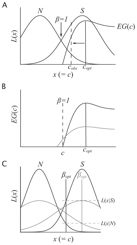
There are two common findings in tasks involving unequal priors and payoffs. First, observers tend to select ‘conservative’ criteria: observed β (β_obs) is closer to 1 than β_opt (Fig. 1A). These effects have been observed in auditory detection (Green & Swets, 1966; Tanner, 1956), line-tilt discrimination (Ulehla, 1966), numerical decision (e.g., deciding whether a randomly selected number represents the height of a man or a woman, Healy & Kubovy, 1981; Kubovy & Healy, 1977), memory tasks (Healy & Kubovy, 1978), and perceptual categorization tasks (Maddox, 2002). Second, the degree of suboptimality of criterion placement when priors are varied tends to differ from that when payoffs are varied. Green and Swets (1966) found that β_obs is closer to optimal with unequal payoffs than with unequal priors. Healy and Kubovy (1981) and Maddox (2002) found the opposite pattern, with β_obs tending to be closer to optimal with unequal priors.

Figure 1.

A. The typical pattern of conservative criterion placement. The internal response (x) to the stimulus is drawn from either the signal (S) or noise (N) distribution. The observer must select a criterion (c) level of x above which they respond, “The signal is present.” The observed criterion, c_obs, is typically closer to that corresponding to β = 1 than the optimal criterion, c_opt, that maximizes expected gain, EG(c). B. Two expected-gain functions that are maximized at the same criterion. The slope of the function in gray is less steep at the neutral criterion corresponding to β = 1 and may induce less of a shift in criterion toward c_opt. C. The effect of underestimation of internal response SD. An observer underestimates (in black) the SD of the actual distributions (in gray). The optimal β (β_opt) in the misestimated distribution corresponds to a criterion closer to the criterion corresponding to β = 1 than the same value of β_opt in the actual distribution.

Various explanations have been suggested for commonly observed patterns of conservative decision criteria including a demand characteristic (Green & Swets, 1966), probability matching (Healy & Kubovy, 1981; Lee & Janke, 1965; Thomas & Legge, 1970), and incorrect assumptions on the part of the researcher regarding the functional form of observers’ internal response distributions (Maloney & Thomas, 1991). Here we focus on four possible sources of the observed suboptimality and address each in turn.

1. The shape of the expected gain function

Maddox and Dodd (2001) suggest that observers, given a set of unequal rewards or priors, shift their criterion away from the position where β = 1 by an amount that depends on the expected increase in reward associated with shifting their criterion to that corresponding to β_opt. Expected Gain (EG) as a function of criterion is calculated as follows:

$$EG(c)=p(S)\mathrm{\Phi }(d^{\prime }-c)V_S+p(N)\mathrm{\Phi }(c)V_N,$$

where d′ is the discriminability of the signal calculated as the difference between the means of the observer’s internal responses to signal-plus-noise and to noise alone divided by the standard deviation of the noise, and Φ is the cumulative standard normal distribution. Φ(d′ − c) is the probability that the observer will respond correctly given the presence of a signal and Φ(c) is the probability of a correct response given noise alone.

Maddox and Dodd (2001) hypothesized that closer-to-optimal shifts in criterion will occur if reward increases more rapidly as the criterion is shifted away from the neutral criterion (Fig. 1B). That is, the steeper the slope of EG(c) at a neutral criterion corresponding to β = 1, the closer to optimal we would expect the observer’s shift in criterion to be. The observer stands to lose little from a suboptimal choice of criterion when EG(c) is relatively flat (i.e., with a slope near 0). In this case the observer is likely to display a pattern of conservatism, maintaining their criterion near that at which β = 1 (see also von Winterfeldt & Edwards, 1982).

Maddox and Dodd (2001) tested observers in a perceptual categorization task with several fixed sets of unequal rewards, penalties, and priors and three different levels of d′. Changing d′ while holding priors and rewards/penalties constant varies the steepness of EG(c). As predicted, they found a trend of closer-to-optimal criterion placement in the d′ conditions with the steepest EG functions.

2. Subjective weighting of rewards

Several authors (Galanter & Holman, 1967; Ulehla, 1966) have suggested that observers’ choices of decision criteria in psychophysical tasks are consistent with a systematic, subjective weighting of the rewards. In calculating the optimal criterion as above, observers do not seem to use the explicit rewards of the task (V_S and V_N ) but rather the utility of the rewards (i.e., u(V_S) and u(V_N )), where u(V ) is a monotonic and concave function of V. As such, they do not choose the response with the maximum expected value (e.g., p(S|x)V_S) but rather, the one with the maximum expected utility (e.g., p(S|x)u(V_S)).

The concept of expected utility originated with Daniel Bernoulli (1954/1738) to explain seemingly irrational patterns in economic decision making not accounted for by expected-value maximization (Fox & Poldrack, 2009). Why, for example, would people consistently prefer $100 in cash to a 50% chance of winning either $200 or nothing? The expected values of both choices are equal ($100), but most people, when offered such a gamble, will choose the sure thing (Allais, 1953, 1979; Kahneman & Tversky, 1979).

According to Bernoulli, a reward represents an increase in wealth. People are innately inclined to judge the impact of an increase in wealth with respect to the current state of wealth. The impact of a reward decreases as the underlying wealth increases so that, for example, $100 seems to be a more substantial amount when the current state of wealth is $0 than when it is $1000.

The utility function, u(·), weights all possible reward values to reflect this innate bias as it manifests in economic decision tasks. To return to the above example, the value of the potential payoff of the gamble, $200, is twice that of the cash payoff, $100. But, assuming a standard form of the utility function:

$$\begin{array}{l}u(V)=V^{\alpha }\\ 0<\alpha <1,\end{array}$$

the utility of $200 is necessarily less than twice the utility of $100. Thus, although the expected values of the two choices are equal: 1 ×$100 = .5 ×$200, the expected utilities are not: 1 × u($100) > .5 × u($200). Hence, most will prefer the $100 cash payoff.

How does this relate to conservative criterion placement? Consider a task in which the prior probabilities for noise and signal stimuli are equal. The optimal criterion is the value corresponding to ${\beta }_{\mathit{opt}}=\frac{V_N}{V_S}$ . The observer calculates the optimal β using the utility of the rewards rather than their explicit values: ${\widehat{\beta }}_{\mathit{opt}}=\frac{u(V_N)}{u(V_S)}$. Assuming the form of the utility function above, β̂_opt will be closer to 1 than β_opt for all values of V_N and V_S. That is, when observers should shift their criteria in response to varied rewards, the observer’s choice of criteria will display a typical pattern of conservatism. Note that this model does not explain conservative criterion shifts in response to varied probability of reward.

3. Subjective weighting of probabilities

People tend to misestimate the relative frequencies of events as they occur in nature (Attneave, 1953; Varey, Mellers & Birnbaum, 1990). This has been particularly well documented in tasks referred to as decision under risk (see Fox & Poldrack, 2009, for a review) of which the monetary gamble above is an example. Risk, in this context, refers to the fact that the outcomes (e.g., winning $200 or $0) are uncertain but the probability of each outcome is known explicitly. In such tasks, observers tend to behave as if they are not using the explicit probabilities but rather subjectively re-weighted ones where the re-weighting takes the form of a systematic over-estimation of low and underestimation of high probabilities (Preston & Baratta, 1948; Tversky & Kahneman, 1992; Gonzalez & Wu, 1999).

The probability weighting function was invoked by Kahnemann and Tversky (1979) to explain biases in economic decision tasks not accounted for by utility theory. Take the following example (cited by Fox & Poldrack, 2009):

• Choice 1.

  1. $3000 for sure

  2. 80% chance of winning $4000

• Choice 2.

  1. 25% chance of winning $3000

  2. 20% chance of winning $4000

Each of the ‘choices’ above is referred to as a lottery. Each reward/probability pair is referred to here as a prospect. The observer selects a prospect from each lottery. People typically choose prospect a, the certain $3000, from the first lottery and prospect b, the lower probability $4000 payoff, from the second. Note, however, that the expected utility of each prospect in lottery 2 equals 1/4 that of each in lottery 1, because each corresponding probability has been multiplied by 1/4. Since scaling the expected utilities does not change their rank order, an expected utility maximizer who prefers a in lottery 1 should also prefer a in lottery 2. The violation of expected utility maximization is attributed to the use of a probability weighting function for which the difference between 1 and .8 is exaggerated relative to the difference between .25 and .20.

What is the effect of probability weighting on decision criteria? Consider a task in which the rewards for correctly detecting signal and noise stimuli are equal. The optimal criterion is the value corresponding to ${\beta }_{\mathit{opt}}=\frac{p(N)}{p(S)}$. We examine the precise form of the probability weighting function, w(·), below, but in its standard form, and assuming that p(N) = 1 − p(S), weighting the prior odds passes them through a power function with exponent γ:

$$\begin{array}{c}\frac{w(p(N))}{w(p(S))}={\left(\frac{p(N)}{p(S)}\right)}^{\gamma }\\ \gamma >0.\end{array}$$

Typical measured values of γ are less than 1 (Fox & Poldrack, 2009). Thus, in a case such as this in which observers select a criterion with varied prior probabilities, the weighted prior odds will be closer to 1 than the true prior odds and observers will display a typical pattern of conservative criterion placement.

4. Misestimation of internal response variability

Finally, conservatism has been linked to a misestimation on the part of the observer as to the variability of their internal response distributions (i.e., X_S and X_N ) (Kubovy, 1977) (Fig. 1C). Having generated an internal response, x, to the stimulus, the observer must calculate its likelihood given that it arose from each distribution (i.e., p(x|S) and p(x|N), respectively). In order to do this, the observer must estimate the standard deviation of the response distributions from a finite sample of exposures to the stimuli.

If an observer underestimates the standard deviation of the internal response, x, the result is that values of the likelihood ratio (i.e., β) for a given value of x will be overestimated for x > 1 and underestimated for x < 1 (Kubovy, 1977). The observer may calculate β_opt correctly, but they will set their criterion response at a value corresponding to β_opt in the misestimated distribution. In terms of the actual underlying distribution, the criterion will be conservative.

The current study

In the current study, we examined observer’s decision criteria in a detection task in which the rewards for correct detection and the probabilities of target occurrence were varied. We compared observers’ decision criteria to the optimal criteria for each set of rewards and probabilities. The rewards and probabilities were varied independently enabling us to examine their differential effects on observers’ choice of criterion. The degree of conservatism when rewards were varied was significantly greater than that found when probabilities were varied.

We tested several hypotheses regarding possible explanations of the overall patterns of conservative criterion placement. First, we asked whether observers’ criteria depend on the slope of EG(c) at the neutral criterion corresponding to β = 1. As noted above, Maddox and Dodd (2001) found a trend for closer-to-optimal criteria with increasingly steepness of the expected gain function. We first sought to replicate that finding.

Second, we ask whether observers select the optimal criterion given their subjectively weighted probabilities and rewards and a misestimation of internal response variance. Note that Maddox and Dodd did consider that their observers were in fact maximizing utility (and not EG(c), per se), but they employed a reward structure for which expected utility is approximately linear. That is, for which the expected gain and expected utility functions are approximately identical. They did not consider subjective weighting of probabilities. Here we explicitly tested whether observers’ use of utility and weighted probability affects their choice of criteria.

Finally, we asked whether observers’ performance is best predicted by a strategy that is independent of the Bayesian optimal one, namely, that observers’ criteria depend only the slope of the subjective utility function (i.e., the product of utility and weighted prior probabilities) at the neutral criterion. The evidence favors this latter hypothesis. We found no relationship between observers’ criteria and the Bayseian optimal criteria. The choice of criterion is predicted by a model that shifts criterion proportionally to the slope of the subjective utility function at a neutral criterion corresponding to β = 1.

Methods

Participants

14 subjects participated in the experiments described below. 6 of these subjects were excluded from running Experiment 3 (‘Main Experiment’ below) and their data were excluded from subsequent analyses due to the adoption of ad hoc strategies in Experiment 2, i.e., performance strategies not accounted for by our model of probability and utility weighting functions. We discuss the criteria for exclusion in the detailed description of the methods for Experiment 2 in the Appendix. A total of 8 subjects (three female) including an author (JFA, ‘Subject 8’ below) completed all three experiments for compensation in the amount of $10 per session for five sessions completed on separate days plus an additional performance-based reward (described below), which ranged from $0–$50. All subjects other than the author were naive to the purpose and background of the study. All had normal or corrected-to-normal vision.

Apparatus

Stimuli were presented on a gamma-corrected, 36 × 27 cm, Sony Multiscan G400 monitor with a resolution of 1600 × 1200 pixels, a refresh rate of 75 Hz, and a mean luminance of 40 cd/m². Eye position was monitored in Experiments 1 and 3 using an SR Research Eyelink1000 desktop eyetracker with a sampling rate of 1000 Hz, controlled using the Eyelink Toolbox Matlab interface (Cornelissen, Peters & Palmer, 2002).

Stimuli

The target stimulus in Experiments 1 and 3 consisted of a 3 deg diameter, 3 cycle/deg Gabor patch in cosine phase (Gaussian envelope SD = 0.66 deg). It always appeared masked by additive Gaussian white noise covering the 3 deg diameter patch. Noise stimuli were generated by randomly sampling each pixel’s value from a normal distribution centered on the monitor’s mean luminance. Noise values were clipped at 3 SDs above and below the mean and then scaled so that the full range of values lay within 1/2 of the display gamut, resulting in a noise SD ≈ 16.5% contrast. Values of the Gabor patch were divided by 1/2 prior to being added to the noise so that the peak signal contrast was at most 50%. Thus, the summed target and noise images always lay within the display gamut. The observer sat at a distance of 57 cm from the monitor. Head position was constrained by a chin rest.

Procedure

Experiment 1 - Contrast Threshold Measurement

As the detectability of a signal (d′) increases, the shift in criterion needed to achieve a particular value of β decreases. Thus at lower d′ levels a greater shift in criterion away from that at which β = 1 is required to achieve β_opt. To determine whether the observer’s choice of criterion depends on d′, we need to examine criterion placement in each of the payoff and prior conditions with signal contrasts corresponding to low and high d′ values.

In Experiment 1, we used a 2AFC detection task to determine the Gabor contrasts corresponding to d′ = .5 and 1 for each subject for use in Experiment 3. Detailed methods for Experiment 1 are given in the Appendix. In summary, peak contrasts corresponding to d′ = .5 and 1 were estimated. These contrast values ranged across subjects from .04 to .08 (d′ = .5), and .06 to .09 (d′ = 1).

Experiment 2 - Weighting Function Parameter Measurement

We hypothesize that criterion placement in the main experiment depends on the subjective weighting of the relevant prior probabilities and rewards, such that the choice of criterion is determined not by expected gain, but by expected utility u(v) with weighted probabilities w(p). We assumed standard functional forms for w and u (Tversky & Kahneman, 1992; Fox & Poldrack, 2009):

$$\begin{array}{c}w(p)=\frac{p^{\gamma }}{{(p^{\gamma }+{(1-p)}^{\gamma })}^{\frac{1}{\gamma }}}\\ u(V)=V^{\alpha },\end{array}$$

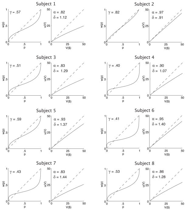
and estimated the values of the parameters, γ and α, (and additional parameters σ and δ described below) by modeling observers’ preferences for particular probability/reward pairs (i.e., prospects) in an economic choice task with the same probability/reward structure as Experiment 3. The estimated parameters for each subject were then used to model criterion choice in Experiment 3. Detailed methods for Experiment 2 are given in the Appendix. To summarize, the estimated parameters and weighting functions for each subject are shown in Fig. 2.

Figure 2.

Probability weighting functions, w(p), and utility functions, u(V ), for each subject, with measured parameters γ, α, and δ.

Experiment 3 - Main Experiment

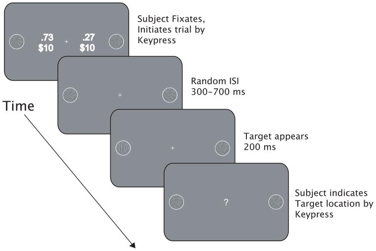
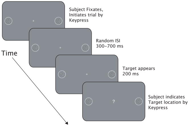
In Experiment 3, subjects performed a 2AFC detection task in which the probability of target occurrence and the rewards for correct detection were varied across alternatives. The trial sequence is shown in Fig. 3. Each block began with a 9-point calibration of the eyetracker. On each trial, the subject fixated a central cross flanked at 10 deg of eccentricity by 3 deg diameter disks containing noise patches. Adjacent to each patch was an indication of the prior probability that the target stimulus would appear at that location and a dollar value giving the reward associated with correctly detecting the target should it appear there. The subject initiated the trial by key press at which time the probabilities and rewards disappeared. Following a random ISI of 300–700 ms, the target stimulus appeared on the left or right side and remained visible for 200 ms. Target contrast corresponded to the low or high threshold contrast as measured in Experiment 1. The target stimulus disappeared leaving only the noise image. Trials in which the subject broke fixation between initiation of the trial and offset of the target were discontinued and rerun later on a randomly selected trial. If fixation was maintained, a small question mark appeared in place of the fixation cross instructing the observer to indicate the side on which the target stimulus appeared by key press. To avoid influencing the subjects’ choice of criterion, no feedback was given in the main experiment.

Figure 3.

Trial sequence for Experiment 3.

The probability/reward structure in all conditions had the following form:

$$p_L,V_L{p}_R,V_R$$

The reward values on the left and right side, V_L and V_R, were always equal when the probabilities on each side were varied and the priors on each side, p_L and p_R, were equal (i.e., p_L = p_R = .5) when the rewards were varied. This allows us to examine the independent effects of varying probabilities and rewards on the subject’s choice of criterion.

Prior probability and reward values were manipulated according to 3 conditions. In the first, ‘Priors’, condition, priors were varied across five levels while rewards were held constant:

$$\begin{array}{l}{p}_R=\{.27,.40,.50,.61,.70\}\\ p_L=1-p_R\\ V_R=V_L=\$10\end{array}$$

The prior values were selected to equate β_opt for each level of the Priors condition with that of the respective level of the other two conditions.

In the second, ‘Rewards’, condition, the priors were held constant while the reward value on the right side was varied across 5 levels relative to the constant reward on the left:

$$\begin{array}{l}{p}_R=p_L=.5\\ V_R=\{\$4,\$7,\$10,\$15,\$23\}\\ V_L=\$10\end{array}$$

The values of V_R were selected to be approximately logarithmically spaced so that changes in value from one level to the next were likely to induce substantial shifts in criterion.

In the third, ‘Equated Priors Condition’, priors were varied across five levels as in the Rewards condition. V_L and V_R were equal but scaled for each level of the priors.

$$\begin{array}{l}{p}_R=\{.27,.40,.50,.61,.70\}\\ p_L=1-p_R\\ V_R=V_L=\{\$6.50,\$7.50,\$10,\$12,\$16\}\end{array}$$

The reward values above are paired with the prior probabilities in the order shown. The scaled rewards equate the slope of EG(c) at the neutral criterion corresponding to β = 1 of each level of the Equated Priors condition with that in the respective levels of the Rewards condition. If we should find significant differences in the degree of conservative criterion choice between the Priors and Rewards conditions (and a similar degree between the Equated Priors and Rewards condition), this will allow us to determine whether the difference in the degree of conservatism with varied priors vs. varied rewards can be attributed to corresponding differences in the slope of EG(c) between the two conditions.

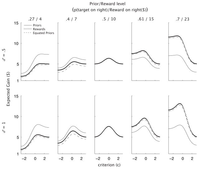
The values of V_L and V_R and p in each of the three conditions were selected such that β_opt for each of the five reward/prior levels was equated across conditions. As explained above, the optimal β is that corresponding to the peak of EG(c), which takes on the following form in a 2IFC paradigm:

$$EG(c)=p_L\mathrm{\Phi }\left(\frac{d^{\prime }}{\sqrt{2}}+c\right)V_L+p_R\mathrm{\Phi }\left(\frac{d^{\prime }}{\sqrt{2}}-c\right)V_R.$$

EG(c) for the five levels of each of the three conditions and d′ level is shown in Fig. 4.

Figure 4.

Expected gain as a function of criterion for each level of the Priors, Rewards, and Equated Priors conditions, and each nominal d′ level. Probabilities and values for the Priors and Rewards conditions are shown above each column.

Experiment 3 was completed in three sessions on separate days. Each session consisted of two blocks of 500 trials each. d′ levels and conditions were blocked. The order in which the d′ levels were run and the order in which each of the three conditions were run within a d′ level were varied randomly between subjects. Subjects completed the three conditions within each d′ level in consecutive blocks. The five levels of each condition within a block were run in sequence from lowest to highest values of p_R and V_R. Pilot experiments showed that running the levels in sequence served to make the task more tractable to the subjects. At the end of the three sessions, a trial was selected at random from all those completed by the subject. If they correctly detected the target on that trial, they received the correspond value of V_L or V_R. Rewards ranged from $0–$16 across subjects.

Results

Overall patterns of conservative criterion placement

Each subject yielded data for three conditions: Rewards, Priors, and Equated Priors, at each of two d′ levels. We fit, by maximum likelihood, a single value of d′ across each of the three conditions at each d′ level, while simultaneously fitting 15 criterion values to the five reward/prior levels within each of the three conditions at each d′ level. Fit d′s ranged from .24 – .63 for the ‘low’ d′ = .5 level, and .72 – 1.32 for the ‘high’ d′ = 1 level. The criteria were converted to β_obs:

$${\beta }_{\mathit{obs}}=e^{\sqrt{2}c{d}^{\prime }}.$$

We tested for position bias (e.g., a bias to choose ‘left’) in the responses across each condition at each d′ level by means of a Pearson’s χ² test. We corrected for significant bias within a condition by multiplying the five levels of β_obs by the value of $\frac{1}{{\beta }_{\mathit{obs}}}$ in the level for which β_obs = 1.

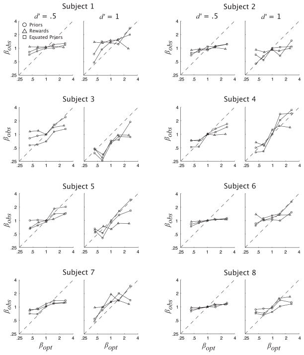
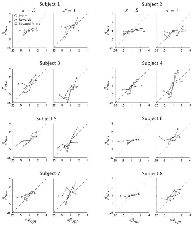
Fig. 5 shows β_obs as a function of β_opt for each subject. Observed β values falling on the diagonal are optimal. Those falling closer to 1 than the diagonal are indicative of conservative criterion placement. Thus, we will summarize the data across the five payoff/prior conditions by the slope of a line fit to these data. A slope of 1 corresponds to ideal behavior, whereas lower slopes imply increasing amounts of conservatism.

Figure 5.

Observed β as a function of optimal β for each subject. Values of β_obs closer to 1 than the the diagonal are conservative

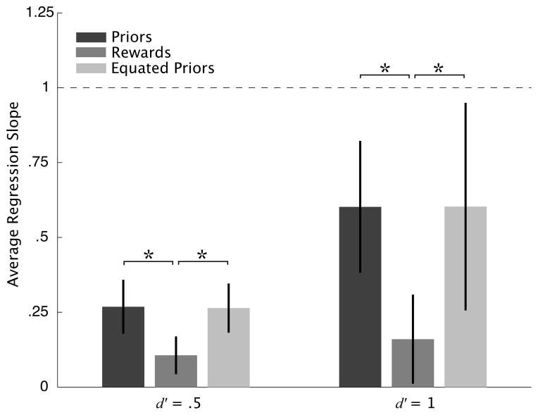
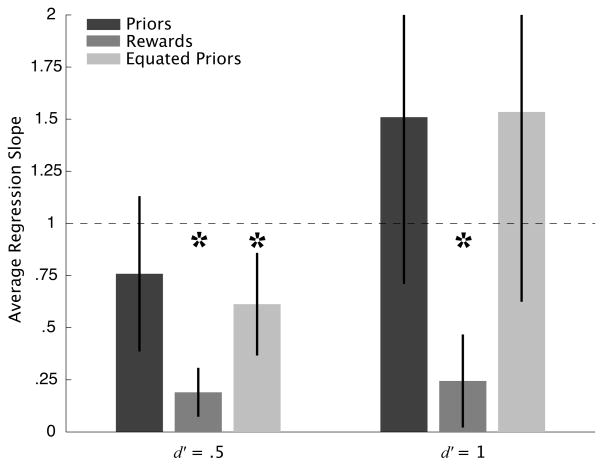
We regressed each subject’s β_obs values onto the corresponding β_opt values for each of the three conditions within each d′ level. Figure 6 shows the average regression slopes across subjects. Two-tailed t-tests show the slope to be significantly less than 1 (p < .05) in all conditions, indicating the predicted overall pattern of conservative criterion placement. Note that there is more error associated with the average slopes, reflecting noisier β_obs, at the higher d′ level. This is due to the fact, noted above, that small changes in criterion result in larger changes in beta when d′ is high. Thus small errors in the measurement of criterion are effectively amplified in the conversion to β at the higher, relative to the lower, d′ level.

Figure 6.

Slopes from the regression of β_obs onto β_opt averaged across subjects. Error bars are 2 SE above and below the mean. All average slopes are significantly different from 1 indicating an overall pattern of conservative criterion placement. All average slopes are significantly greater than 0 indicating a significant effect of the levels of the prior probabilities and rewards in each condition. Asterisks indicate a significant difference between conditions at p < .05.

Next we ask whether the levels of each condition brought about a significant change in the subjects’ β_obs, i.e., that the observed suboptimality is not due to the subjects merely ignoring the probabilities and rewards. We assume the slopes to be equal to or greater than 0 (since slopes < 0 would infer a subjective inversion of probabilities and rewards) and compare the average slopes to 0 using one-tailed t-tests. The average slopes in all conditions are significantly greater than 0 (p < .05) suggesting a significant effect of the levels for each condition.

We compared slopes between conditions and d′ levels by means of a 3 × 2 repeated-measures ANOVA. Results show a significant main effect of d′ level on regression slope (F(1, 7) = 8.29, p < .05), a significant main effect of condition, (F(2, 14) = 8.37, p < .05), and a significant interaction between d′ level and condition (F(2, 14) = 4.84, p < .05), reflecting the relative increase in the slope in the Priors and Equated Priors conditions at the higher d′ level. That slopes are significantly greater at the higher d′ level is to be expected as, again, smaller changes in criterion are needed to achieve the optimal criterion as d′ increases. That slopes for the Priors and Equated Priors conditions appear to be significantly greater than those in the Rewards is addressed next.

Having found significant effects of condition and d′ level, we can compare the average slopes for the regression of β_obs onto β_opt across conditions by means of two-tailed dependent-sample t-tests. The results are shown in Fig. 6. Within each level of d′, regression slopes for the Priors and Equated Priors are significantly closer to optimal than those of the Rewards condition. Slopes for the Priors and Equated Priors conditions do not differ significantly. This suggests that the relatively lower level of conservatism observed in the conditions in which the prior probabilities are varied, over those in which rewards are varied, is not due to a difference in the shape of the respective expected gain functions (since expected gain in the Equated Priors condition is nearly equal to that in the Rewards condition). We address this further in the Discussion section.

The cost of conservative criterion placement

We have found that observers place their criteria conservatively. We next ask whether suboptimal choice of criterion resulted in a significant cost to the observers. We computed the cost of the suboptimal criterion placement for each level of the Payoffs, Priors, and Equated Priors conditions, within each d′ level. Cost is calculated as the difference between maximum EG (given the optimal criterion, c_opt) and the observer’s EG (given their observed criterion, c_obs). We normalized cost relative to the expected gain of an unshifted criterion (i.e., c = 0, corresponding to β_obs = 1):

$$\text{normalized}\text{cost}=\frac{EG(c_{\mathit{opt}})-EG(c_{\mathit{obs}})}{EG(c_{\mathit{opt}})-EG(c=0)}.$$

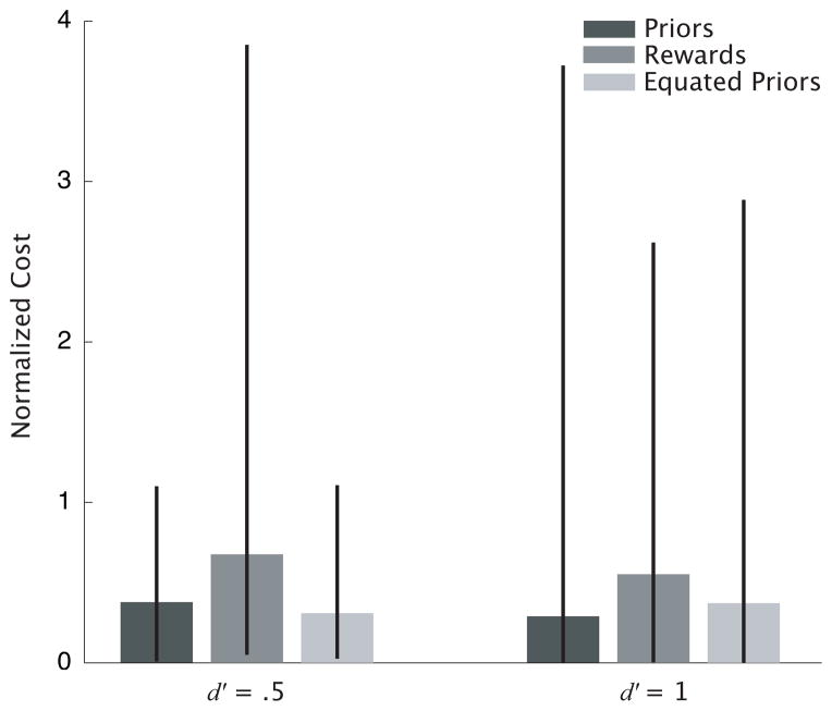
Fig. 7 shows the median normalized cost across the levels of each condition (excluding those for which c_opt = 0) and across subjects. Error bars show the central 95th percentile range of the median normalized cost. The cost is significantly greater than 0 in all conditions. Suboptimal choice of criterion resulted in significant and, in many cases, substantial non-zero costs in all conditions.

Figure 7.

Median normalized cost (see text), calculated across subjects, for each condition and d′ level. Error bars show the central 95th percentile range. Normalized cost in all conditions is significantly greater than 0.

We have found suboptimal criterion placement on the part of the observers and linked the suboptimal criteria to significant decrements in the observers’ expected gain for the task. We now investigate several potential causes of the suboptimal choice of criterion.

Effect of the shape of EG(c)

Here we assume that the observer’s ‘baseline’ criterion in the task corresponds to β = 1, i.e., the optimal criterion when rewards and priors are equal. We assume that the observer has knowledge of the optimal criterion given the altered rewards and probabilities and that the slope of EG(c) at a neutral, unshifted criterion is the driving force for the resulting shift from the neutral to the chosen criterion (Maddox & Dodd, 2001). We define EG′(c = 0) to be the value of the slope of EG(c) at the neutral criterion corresponding to β = 1:

$$E{G}^{\prime }(c=0)=p_L\varphi \left(\frac{d^{\prime }}{\sqrt{2}}\right)V_L-p_R\varphi \left(\frac{d^{\prime }}{\sqrt{2}}\right)V_R,$$

where ϕ is the standard normal density.

To measure the degree to which observers shift their criterion as a function of EG′(c = 0), we calculated the magnitude of the criterion shift in terms of β, away from β = 1, normalized by the optimal criterion shift:

$$\text{normalized}\text{shift}=\frac{{\beta }_{\mathit{obs}}-1}{{\beta }_{\mathit{opt}}-1}.$$

We regressed normalized shift onto |EG′(c = 0)|, on the data pooled across subjects. Having found significant effects of condition and d′ on the change in β_obs, we regressed normalized shift separately across the levels of the Rewards and the two Priors conditions, for each d′ level. Because both normalized shift and the slope of the EG function depend on d′ as measured for each subject in the main experiment, we use a model, Total Least Squares (TLS) regression (Markovsky & Van Huffel, 2007; Petras & Bednarova, 2010), that accounts for the error in both variables. We achieve unit-invariance of the regression fit by normalizing the values of |EG′(c = 0)| and normalized shift by their respective SDs prior to regressing. Outlying values of |EG′(c = 0)| were identified by calculating their studentized residuals (Cook, 1982) and eliminated prior to regressing.

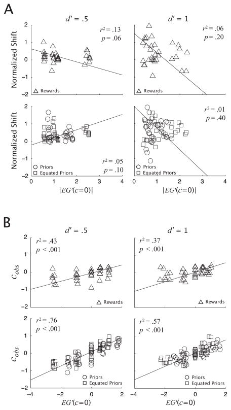
Fig. 8A shows normalized shift as a function of |EG′(c = 0)| with the TLS regression lines. The regression slopes are not significantly different from zero and r² values are low. The results suggest that the steepness of the EG function has no effect on the magnitude of the shift in criterion away from β = 1 relative to the optimal criterion.

Figure 8.

A. Normalized shift (see text) as a function of the absolute value of the slope of EG(c) at the neutral criterion corresponding to β = 1, for all subjects. The top row shows the Rewards condition. The bottom row shows the Priors and Equated Priors conditions. The across-subject average TLS regression lines (scaled to the original units) are shown. B. c_obs as a function of the slope of EG(c) at the neutral criterion (c = 0) with the TLS regression lines. All other details as in A.

Next, we ask whether there is a relationship between the slope of the EG function and the value of the observed criterion, independent of the optimal criterion. That is, we hypothesize, as the results above suggest, that the observer shifts their criterion in direct proportion to the slope of the EG function at the neutral criterion, and not in proportion to the optimal β. We assume that the observer sets their criterion in units of the internal response to the stimulus, and not in units of β (a non-linear function of the stimulus response). Thus, we performed linear regression of c_obs directly onto EG′(c = 0) using the same method as above and tested for a regression slope significantly different from 0. Fig. 8B shows the results of the TLS regression. Regression slopes are significantly different from 0 for both conditions and d′ levels and r² values are moderate to high. The results indicate a strong linear relationship between the slope of the EG function and c_obs, independent of c_opt.

We have found that the steepness of the expected gain function at a neutral criterion is predictive of the absolute magnitude of the observer’s criterion shift. Next we examine the effect of weighting probabilities and rewards on the choice of criterion.

Effect of weighted probabilities and rewards

Here we hypothesize that, following exposure to the signal stimulus, the observer calculates the subjective utility, SU, of choosing the left or right target position given the prior probabilities, p, and rewards, V, on each side, L and R, for the current condition and d′ level:

$$\begin{array}{c}SU(x)=w(p_L)\mathrm{\Phi }\left(\frac{x+\frac{d^{\prime }}{\sqrt{2}}}{{\sigma }_w}\right)u(V_L)+w(p_R)\mathrm{\Phi }\left(\frac{x-\frac{d^{\prime }}{\sqrt{2}}}{{\sigma }_w}\right)u(V_R)\\ w(p)=\frac{p^{\gamma }}{{(p^{\gamma }+{(1-p)}^{\gamma })}^{\frac{1}{\gamma }}}\end{array}$$

where u(V_L) = V_L^α, u(V_R) = δV_R^α in the Rewards condition when its value is changing relative to V_L, and u(V_R) = V_R^α in the Priors and Equated Priors conditions when its value equals that of V_L.

Note that in this model the observer weights only the explicitly presented probabilities, p_L and p_R, and not the implicit likelihood of the internal response or posterior probability of getting the reward. This is consistent with the observation that explicit probabilities are subject to the type of nonlinear weighting described by prospect theory and implicit “probabilities from experience” are not (Hertwig, Barron, Weber & Erev, 2004).

We assume that the observer underestimates the standard deviation of the internal signal-response-difference distribution. σ_w (< 1) is the observer’s misestimated standard deviation. We further assume that observers choose the criterion, wc_opt, corresponding to wβ_opt, the optimal β given the weighted probabilities and rewards:

$$w{\beta }_{\mathit{opt}}={\left(\frac{p_L}{p_R}\right)}^{\gamma }{\left(\frac{V_L}{V_R}\right)}^{\alpha }=\frac{\varphi \left(\frac{x-\frac{d^{\prime }}{\sqrt{2}}}{{\sigma }_w}\right)}{\varphi \left(\frac{x+\frac{d^{\prime }}{\sqrt{2}}}{{\sigma }_w}\right)}.$$

α and γ in the above equation refer to the values measured for each subject in Experiment 2. σ_w was fit to the data by maximum likelihood using the following iterative procedure: Given an initial estimate of σ_w, we calculated the SU(c) of choosing the left and right side as above, for each of the five levels, i, of each reward/prior condition, j, and d′ level, k. Note that the optimal criterion signal-response-difference, x = wc_opt, corresponds to that at which the SUs for each side are equated. Thus wc_opt can be derived by solving:

$${wc}_{op{t}_{i,j,k}}=\underset{x}{arg}\left(w(p_{L_{i,j}})\mathrm{\Phi }\left(\frac{x+\frac{d_k^{\prime }}{\sqrt{2}}}{{\sigma }_w}\right)u(V_{L_{i,j}})-w(p_{R_{i,j}})\mathrm{\Phi }\left(\frac{x-\frac{d_k^{\prime }}{\sqrt{2}}}{{\sigma }_w}\right)u(V_{R_{i,j}})=0\right).$$

In other words, wc_opt corresponds to the zero-crossings of the above function of x, which was solved using MATLAB function fzero. The binomial log likelihood of the resulting estimate of σ_w was then calculated given the estimated probability of a correct response, p̂(c_L) and p̂(c_R), on the left and right sides, respectively:

$$\begin{array}{l}\widehat{p}(c_{L_{i,j,k}})=\mathrm{\Phi }\left(\frac{\frac{d_k^{\prime }}{\sqrt{2}}+{wc}_{op{t}_{i,j,k}}}{{\sigma }_w}\right)\\ \widehat{p}(c_{R_{i,j,k}})=\mathrm{\Phi }\left(\frac{\frac{d_k^{\prime }}{\sqrt{2}}-{wc}_{op{t}_{i,j,k}}}{{\sigma }_w}\right),\end{array}$$

summed across conditions and d′ levels, and maximized yielding the best estimate of σ_w for each subject.

As explained in the introduction, weighting probabilities and rewards has the effect of pushing wβ_opt closer to 1 than the unweighted β_opt. Thus, we expect that β_obs, though exhibiting conservatism in terms of the unweighted EG functions and veridical internal response distributions (i.e. with σ = 1), will be optimal given SU with misestimated noise, σ_w. We regressed β_obs onto wβ_opt. Fig. 9 shows β_obs as a function of wβ_opt with corresponding values of σ_w and Fig. 10 shows the linear regression slopes averaged across subjects. t-tests show the average slopes to be significantly less than 1 in three out of six cases indicating conservative criterion placement. Slopes in the Priors conditions for both d′ levels and Equated Priors condition for d′ = 1 are not significantly different from 1 indicating optimal criterion placement. However, note that average slopes are greater than 1 in the Priors and Equated Priors conditions (for d′ = 1) for subjects 1 and 3 – 7. Thus, the fact that the average slopes are not significantly different from 1 for those conditions does not suggest that subjects are selecting their criteria in an ‘optimal’ fashion with respect to the weighted optimal criteria. c_obs tends to ‘overshoot’ wc_opt in these cases.

Figure 9.

Observed β as a function of weighted optimal β (see text) for each subject. Values of β_obs closer to 1 than the the diagonal are conservative.

Figure 10.

Slopes from the regression of β_obs ontp wβ_opt averaged across subjects. Error bars are 2 SE above and below the mean. Asterisks indicate that the average slopes are significantly different from 1 at p < .05.

In sum, we hypothesized that subjects’ β_obs would be optimal with respect to wβ_opt. Our results show that this is not the case. We have found that β_obs is suboptimal relative to the Bayesian optimal β both in the case where probabilities and rewards are treated veridically (β_opt) and in the case where we factor in weighted probabilities and rewards (wβ_opt) and allow for an underestimation of internal response variability (σ_w). We next examine the effect of the shape of SU(c) on the choice of criterion.

Effect of the shape of SU(c)

Here we assume that the observer weights prior probabilities and rewards and uses them to calculate SU(c). The observer calculates the slope of SU(c) at a neutral criterion corresponding to β = 1 and shifts the criterion relative to wβ_opt in proportion to the slope. We do not assume that the observer sets their criterion to that corresponding to wβ_opt as above. The observer’s estimate of the internal response variance is assumed to equal 1 in all that follows. The form of SU(c) on a given trial is thus:

$$SU(c)=w(p_L)\mathrm{\Phi }\left(c+\frac{d^{\prime }}{\sqrt{2}}\right)u(V_L)+w(p_R)\mathrm{\Phi }\left(c-\frac{d^{\prime }}{\sqrt{2}}\right)u(V_R),$$

and the slope of SU(c) at β = 1 is given by:

$$S{U}^{\prime }(c=0)=w(p_L)\varphi \left(\frac{d^{\prime }}{\sqrt{2}}\right)u(V_L)-w(p_R)\varphi \left(\frac{d^{\prime }}{\sqrt{2}}\right)u(V_R).$$

We calculated the normalized criterion shift relative to the weighted optimal criterion as above:

$$\text{normalized}\text{shift}=\frac{{\beta }_{\mathit{obs}}-1}{w{\beta }_{\mathit{opt}}-1},$$

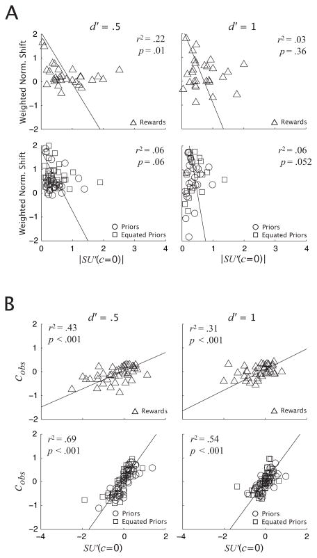
and compare this to SU′(c = 0) by means of TLS regression as above. Fig. 11A shows normalized shift as a function of SU′(c = 0) across subjects, separately for the Rewards and two Priors conditions within each d′ level. The slope is significantly different from 0 in the Rewards condition at the low d′ level only. As with EG′, r² values are low. All slopes are negative reflecting a larger increase in wβ_opt – 1 relative to β_obs – 1 going from low to high levels of the priors and rewards; in other words, a failure of β_obs to keep pace with shifts in β_opt. As with the unweighted EG(c), the steepness of the SU(c) function does not predict the magnitude of the shift in criterion away from β = 1, relative to the weighted optimal criterion.

Figure 11.

A. Normalized shift (see text) as a function of the absolute value of the slope of SU(c) (i.e., expected utility calculated using weighted priors) at the neutral criterion corresponding to β = 1, for all subjects. The top row shows the Rewards condition. The bottom row shows the Priors and Equated Priors conditions. The across-subject average TLS regression lines (scaled to the original units) are shown. B. c_obs as a function of the slope of SU(c) at the neutral criterion (c = 0) with the TLS regression lines. All other details as in A.

Next, we ask whether there is a relationship between the slope of the SU(c) and the value of c_obs, independent of the optimal criterion. As above with EG′(c = 0), we regressed c_obs directly onto SU′(c = 0) and tested for a regression slope significantly different from 0. Fig. 11B shows the results of TLS regression. Regression slopes are significantly different from 0 in all cases and r² values are moderate to high. As with EG, the results indicate a strong linear relationship between the slope of the SU function and c_obs, independent of c_opt.

We have found that the slope of EG(c) and SU(c) are both predictive of β_obs. We would like to compare the ability of each computation of expected value to predict β_obs. Each differs only in the values of the probability weighting and utility function parameters used. In calculating EG(c), α, γ, and δ are effectively set to 1. In calculating SU(c) they are set to the values measured in Experiment 2. The parameters are constants in each case and so each regression model has the same number of free parameters. Thus we can simply compare the likelihood of the TLS regression fits of EG(c) and SU(c) to β_obs. The log likelihood of the fit is given by:

$$log\text{likelihood}=-\frac{N}{2}(ln(2\pi )+ln({\sigma }_r^2)+N-1),$$

where N is the number of data points being fit and ${\sigma }_r^2$ is the orthogonal residual variance.

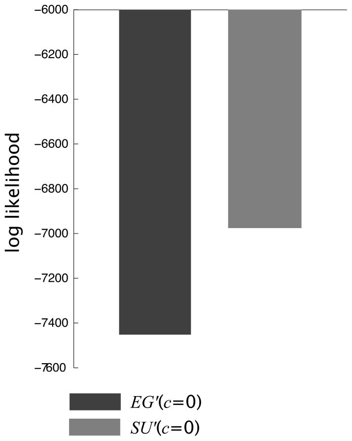
Fig. 12 shows log likelihood of the fits summed across conditions and d′ levels. Larger values indicate a more predictive fit to the data. The likelihood of SU(c) is greater and thus we conclude that the slope of SU(c) at the neutral criterion is a better predictor of β_obs than that of EG(c).

Figure 12.

Log likehood of the TLS regression of c_obs onto the slope of the expected gain function, EG′ (c = 0), and the subjective utility function, SU′ (c = 0), at the neutral criterion. Values closer to 0 indicate the more predictive fit. SU′ (c = 0) is more predictive of c_obs.

Discussion

We conducted a 2AFC detection task in which the probability of target occurrence and the reward for correct detection were varied across alternatives. Observers’ criteria for each level of the probabilities and rewards were conservative. That is, their corresponding β fell closer to 1 than the optimal β.

We explored several possible explanations for the conservative criterion placement. We did not find a relationship between the Bayesian-optimal criteria and the subjects’ criteria or evidence that subjects’ conservatism resulted from a misestimation of internal response variance. The Bayesian-optimal criteria, assuming weighted probabilities and rewards and a misestimation of internal response variance, consistently underestimated the observed criteria. Nor was there a significant correlation between the observers’ shift in criterion relative to the optimal one and the slope of unweighted, EG(c), or weighted, SU(c), expected value functions. We did find significant linear relationships between the observed criteria and the slope of both EG(c) and SU(c), independent of the optimal criteria. The slope of SU(c) was more predictive than that of EG(c).

We conclude that observers in our task selected their criteria, without regard to the Bayesian-optimal one, solely on the basis of the steepness of the subjective utility function, at the neutral criterion corresponding to β = 1. In other words, in a perceptual task such as this in which people are given a choice between alternatives with different values and probabilities, people will choose based on a calculation of how much they stand to gain (per amount of criterion shift) by changing their strategy away from the neutral criterion. This increase in gain is estimated using subjectively distorted prior probabilities and values.

We found that subjects’ criteria were closer to optimal when the prior probabilities were varied than when rewards were varied. As noted, this result has been observed previously (Healy & Kubovy, 1981; Maddox, 2002). It is consistent with the adoption of competing strategies on the part of the observers. Namely, to maximize gain on one hand and to maximize accuracy on the other (Markman, Baldwin & Maddox, 2005; Maddox & Dodd, 2001; Maddox & Bohil, 1998a). The observer who is attempting to maximize accuracy will set their criterion at that which maximizes hits and minimizes false alarms and which effectively matches the probability of target occurrence for each alternative. When rewards are varied and the probability of each alternative is equal, this strategy will result in a criterion close to 0 (β = 1), i.e. that at which the probability of being correct is the same for each alternative. When the prior probabilities are varied (and rewards held constant), the same strategy will result in a greater shift in criterion away from 0. We assert here that the observers seem to be using both reward and accuracy maximizing strategies since changing the rewards in our task brought about a significant shift in criterion. It is also worth noting that models that predict criterion as a function of the slope of the EG and SU functions do very well for both Priors and Reward conditions. The influence of rewards on criterion shift may explain why criteria in the two Priors conditions fall short of optimal. A simple probability-matching strategy would suffice to maximize accuracy (and achieve optimal criteria), but subjects seem to be accepting a higher degree of error, which is consistent with a competing reward-maximizing strategy.

Further confirmation of the dependence of criterion choice on weighted probabilities and rewards may come from altering people’s weighting functions and looking for an associated change in the chosen criterion for a given set of probabilities and rewards. In this paper, we have addressed a fundamental assertion of Prospect Theory, that people’s preferences depend on the weighting of both probabilities and rewards. A second, equally important aspect of Prospect Theory is that a person’s preference for a lottery depends on how it is framed (Tversky & Kahneman, 1986). For example, an observer’s preference can be altered by posing lotteries in terms of potential losses rather than potential rewards, by summing a lottery’s component prospects in order ‘hide’ its stochastic dominance (i.e., the fact that it possesses a higher probability of paying off a higher reward than all others), and by imposing ‘endowments’ that effectively raise the reference point of the utility function. Prospect Theory exposed these effects as violations of a rational decision making process. An experimenter, however, may capitalize on them in order to observe the subsequent effect on decision criteria. If probability and reward weighting functions are flexible, and if their effect on decision criteria proves robust, this also implies that they could be altered in the service of improving performance in the type of critical detection task described in the Introduction.

The conclusion that observers shift their criteria in proportion to the subsequent change in expected value suggests that shifting entails a cost. Future research may examine the nature of this cost. Does it, for example, entail a risk of lowering expected value by altering a hitherto successful strategy? Or does shifting carry with it a transaction cost (Williamson, 1981) such that it is costly in its own right independent of expected value? The cost may also be in terms of the increase in misses or false positives incurred by a criterion shift. Whereas, in our study, we model an ideal observer as one that maximizes expected value, our observers may have a conflicting goal of maximizing accuracy, as mentioned above. The reluctance to shift may reflect this conflict.

Finally, we address potential weaknesses of the study. First, the inclusion of the author as a subject is of concern since knowledge of optimal strategies, e.g. merely calculating the expected gain of all presented prospects in Experiment 2, or adoption of an intentionally suboptimal strategy could potentially skew the results. To confirm that Subject 8’s data don’t create statistical artifacts that may bias our conclusions, we performed the ANOVA for a significant effect of d′ and condition on the regression slope of observed β vs. optimal β, 8 times, systematically leaving out 1 of the 8 subjects on each run. The results for each run were the same. We found significant main effects of d′ and condition regardless of which subject was excluded. However, the interaction between d′ and condition obtains only when all 8 subjects are included, i.e., if any 1 subject is left out the interaction is not significant. Since β effectively normalizes criterion with respect to d′ and since the optimal β is the same across subjects in the above regression, and since the overall conclusions regarding EG(c) and SU(c) depend largely on these, we think this is a good indication that Subject 8’s criteria and d′ don’t represent outlying values that skew our conclusion.

Next, several studies have suggested that attaching value to a target enhances attention to it (Anderson, Laurent & Yantis, 2011; Libera & Chelazzi, 2006). It is well known that enhanced spatial attention has the effect of increasing sensitivity to contrast-defined targets (Carrasco, 2011, 2006). Thus, it may be that attaching different values to our targets led to an attentional effect that altered observers’ d′ values from those measured in Experiment 1 and hence, our estimate of the optimal criteria in the main experiment.

In addition, we have assumed here that only explicitly presented probabilities are subject to non-linear weighting. The observers’ implicit estimates of internal response likelihood (i.e. p(x|S) and p(x|N)) were assumed to be un-weighted. This is not necessarily the case. The observer must estimate the likelihood of a response on a given trial based on the distribution of responses across previous trials. Such ‘probabilities from experience’ can be subject to a weighting such that the probabilities of rare values are underestimated (Hertwig, Barron, Weber & Erev, 2004), a pattern opposite to that observed with explicit probabilities. If p(x|S) and p(x|N) were subjectively weighted in this way, the observer’s weighted estimated β, wβ, for a given value of x would be further from 1 than the unweighted β. The observer, attempting to set their criterion at a value of x such that wβ = wβ_opt, would compensate by selecting a value of x closer to β = 1. That is, β_obs would be conservative. If β_obs is itself subject to non-linear weighting in this way, this may explain our observation that wβ_opt underestimates β_obs. Future research may attempt to measure observers’ weighting parameters for ‘probabilities from experience’ and investigate their effect on observed values of β.

Appendix

Experiment 1 - Contrast Threshold Measurement

Experiment 1 was completed in a single session. We used a 2AFC detection task to determine the Gabor contrasts corresponding to d′ = .5 and 1 for each subject for use in Experiment 3. The trial sequence is shown in Fig. 13. Each block began with a 9-point calibration of the eyetracker. On each trial, the subject fixated a central cross flanked at 10 deg of eccentricity by 3 deg diameter disks containing noise patches. They initiated the trial by key press. Following a random ISI of 300–700 ms, the target stimulus appeared on the left or right side, chosen at random, and remained visible for 200 ms. The target stimulus disappeared leaving only the noise image (the same noise image was used throughout the trial). Trials in which the subject broke fixation between initiation of the trial and offset of the target were discontinued and rerun later on a randomly selected trial. If fixation was maintained, a small question mark appeared in place of the fixation cross instructing the observer to indicate the side on which the target stimulus appeared by key press. Subjects received auditory feedback on each trial in the form of a high tone for a correct and a low tone for an incorrect response.

Figure 13.

Trial sequence for Experiment 1.

Stimulus contrast on each trial was determined by one of two staircases (1-up/3-down, 1-up/2-down) selected at random independently of the side on which the target appeared. Contrasts were sampled from 25 logarithmically spaced values ranging from .01 – .95. The initial stepsize for each staircases was three. The step size was decreased by one after the first and second reversals. Each subject completed two blocks of 200 trials each in a single session. The staircases were initiated at the beginning of each block. The first block served to stabilize the subjects’ performance in the task. Only the 200 trials of the second block (100 per staircase) were analyzed. Each subject’s data were pooled across the two staircases. Probability correct as a function of contrast was modeled using a Weibull function fit to the data by maximum likelihood. Peak contrasts corresponding to d′ = .5 and 1 were estimated from the fit curve. These contrast values ranged from .04 to .08 (d′ = .5), and .06 to .09 (d′ = 1).

Experiment 2 - Weighting Function Parameter Measurement

As mentioned above, observers’ preferences for a reward, V, given the probability of receiving it, p, deviate from those predicted by assuming the observer maximizes expected gain. They are well predicted by a model that assumes non-linear weighting of probabilites, w(p), and rewards, u(V ). Here we assume standard functional forms for w and u (Tversky & Kahneman, 1992; Fox & Poldrack, 2009):

$$\begin{array}{l}w(p)=\frac{p^{\gamma }}{{(p^{\gamma }+{(1-p)}^{\gamma })}^{\frac{1}{\gamma }}}\\ u(V)=V^{\alpha },\end{array}$$

and estimate the values of the parameters, γ and α, by modeling observers’ preferences for particular probability/reward pairs, i.e., prospects.

On each trial, observers were presented with a choice between a pair of prospects of the form (Fig. 14):

$$(p_i,X;(1-p_i),0)\text{or}((1-p_i)V_{i,j};p_i,0),$$

where X is a value that is held constant across trials, and V is a value that changes on each trial. They were instructed to choose which ‘gamble’ they would prefer. It was explained to the subjects that the dollar values, X and V, were amounts they could actually win and that the probabilities represented the chance of “blindly reaching into a box containing a huge number of lottery tickets, some with the dollar value on them, some with $0 on them, and selecting a winning ticket.” All subjects indicated that they understood the task. Upon completion, a prospect was selected at random from all those chosen by the subject and the outcome of the gamble was generated pseudo-randomly by computer. The subject received the payoff, which ranged from $0–$50 across subjects.

Figure 14.

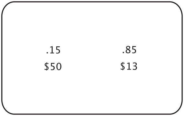
Sample display from Experiment 2. See text for description.

On each trial, the value of p_i was selected at random from: {.1, .18, .28, .4}. The value of X was fixed at $50. For each value of p_i, five values of V_i,j were employed corresponding to five values of the psychometric function, {.2, .35, .5, .65, .8}, that gives probability, P(choose V ), of choosing the prospect containing V_i,j (as a function of only V_i,j) given the current estimates of the parameters γ and α.

An additional parameter, δ, was added to account for patterns of choice observed in piloting Experiment 2. In piloting the experiment, we found that subjects’ choices were consistent with an additional weighting of the changing value, δV_i,j (for δ > 1), such that increases in its value are subjectively exaggerated. Experiment 2 results in data to which four psychometric functions (each corresponding to one of the four values of p_i), giving P(choose V ) as a function of V_i,j, are fit. The parameters γ and α determine the relative spacing of the four psychometric functions. Increasing values of δ shift the four functions uniformly toward lower values of V_i,j. The addition of δ led to a substantial reduction in the error of the fits. The method for selecting the values of V_i,j is explained below.

Under prospect theory, as modified by the additional δ parameter, the subject will choose the lottery containing V_i,j when:

$$w(1-p_i)u(\delta V_{i,j})>w(p_i)u(X).$$

Putting this in terms of the unweighted value of V_i,j and rearranging the terms, we obtain:

$$\text{choose}V\text{when}:V_{i,j}>{\left(\frac{p_i}{1-p_i}\right)}^{\frac{\gamma }{\alpha }}\frac{X}{\delta }$$

and equivalently:

$$\text{choose}V\text{when}:\frac{V_{i,j}}{{\left(\frac{p_i}{1-p_i}\right)}^{\frac{\gamma }{\alpha }}\frac{X}{\delta }}>1$$

and taking the log of each side:

$$\text{choose}V\text{when}:ln(V_{i,j})-ln\left({\left(\frac{p_i}{1-p_i}\right)}^{\frac{\gamma }{\alpha }}\frac{X}{\delta }\right)>0.$$

We assume that the subject’s internal representation of the difference on the left of the inequality is corrupted by noise drawn as a random sample from a normal distribution with mean = 0. Furthermore, we assume under Weber’s law that the SD of the distribution for each value of i is equal in log value. The probability of choosing the lottery containing V_i,j is thus given by:

$$P_i(\text{choose}V)=\mathrm{\Phi }\left(\frac{ln(V_{i,j})-ln\left({\left(\frac{p_i}{1-p_i}\right)}^{\frac{\gamma }{\alpha }}\frac{X}{\delta }\right)}{\sigma }\right).$$

Initial values for V_i,j were derived by choosing five values for P_i(choose V ) that span the psychometric function: {.2, .35, .5, .65, .8}, and then solving:

$$V_{i,j}={\left(\frac{p_i}{1-p_i}\right)}^{\frac{\gamma }{\alpha }}\frac{X}{\delta }exp\left(\sigma {\mathrm{\Phi }}^{-1}(P_i(\text{choose}V))\right)$$

with parameter values: α = .65, γ = .5, and σ = .2 chosen to represent reasonable parameter estimates given a survey of estimates across many studies (Fox & Poldrack, 2009), and the initial value of δ set to 1. The maximum value of V_i,j never exceeded $50 so that the prospect containing V_i,j was never stochastically dominant.

Prospects were presented using the method of constant stimuli. Values of p_i and their corresponding V_i,j were chosen at random from each of the four probability and five value levels with equal numbers of trials from each level (i.e., five trials per probability/value pair) within each block. To avoid stereotyped responses, displayed values of V_i,j were randomly jittered by an amount no more than ±1/4 of the minimum difference between any two values of V for the given block. To avoid response-side bias, the side with the lottery containing V was selected at random on each trial. Subjects indicated their preferred prospect on each trial by key press.

Subjects completed four 100-trial blocks in a single session. At the end of each block, estimated α, γ, σ, and δ were fit to the binned data from all preceding blocks by maximum likelihood where the estimated probability of choosing the prospect containing V_i,j is given by:

$${\widehat{P}}_i(V_{i,j})=\mathrm{\Phi }\left(\frac{ln(V_{i,j})-ln\left({\left(\frac{p_i}{1-p_i}\right)}^{\frac{\gamma }{\alpha }}\frac{X}{\delta }\right)}{\sigma }\right).$$

The resulting estimates of α, γ, σ, and δ were used to select new values of V_i,j for use in the subsequent block. The fit parameters and weighting functions for each subject are shown in Fig. 2.

All subjects were debriefed following the task as to any strategy they may have employed. One subject indicated that they had merely calculated the expected gain of the prospects. Their data were excluded from the analyses and they did not continue with Experiment 3. In addition, five subjects employed ad hoc strategies for which the model above cannot account. Two subjects chose the lottery containing the higher probability and lower value, V, on more than 90% of trials, a strategy which effectively ignores values. Three subjects chose the lottery containing the constant value X on the majority of trials when the probabilities associated with V and X were nearly equal, i.e. when p = .4, but seemed to employ more typical weightings of probabilities and values for other probability levels. These subjects’ data were also excluded and their participation was discontinued since the model above cannot account for these strategies nor can we make valid estimates of decision criteria in the subsequent experiment if such strategies are being employed. Note that these subjects were excluded not because they used strategies that are alternative to calculating the subjective utility of the prospects. Rather, we assume that all subjects, under general circumstances, subjectively weight probabilities and values in the way described by prospect theory. The ad hoc strategies employed simply make it impossible to measure their weighting functions without increasing the complexity of the model to account for idiosyncratic strategies.

References

- Allais M. Le comportement de l’homme rationel devant le risque, critique des postulates et axiomes de l’ecole americaine. Econometrica. 1953;21:503–546. [Google Scholar]
- Allais M. The so-called Allais paradox and rational decisions under uncertainty. In: Allais M, Hagen O, editors. Expected Utility Hypothesis and the Allais Paradox. Dordrecht, The Netherlands: Reidel Publishing Company; 1979. pp. 437–681. [Google Scholar]
- Anderson B, Laurent P, Yantis S. Value driven attentional capture. Proceedings of the National Academy of Sciences. 2011;108:10367–10371. doi: 10.1073/pnas.1104047108. [DOI] [PMC free article] [PubMed] [Google Scholar]
- Attneave F. Psychological probability as a function of experienced frequency. Journal of Experimental Psychology. 1953;46:81–86. doi: 10.1037/h0057955. [DOI] [PubMed] [Google Scholar]
- Bernoulli D. Exposition of a new theory of risk [translation by l. sommer of d. bernoulli, 1738, specimen theoriae novae de mensura sortis, papers of the imperial academy of science of saint peterburg, 175–192] Econometrica. 1954/1738;22(1):23–36. [Google Scholar]
- Carrasco M. Covert attention increases contrast sensitivity: Psychophysical, neurophysiological, and neuroimaging studies. In: Martinez-Conde S, Macknik S, Martinez L, Alonso J, Tse P, editors. Visual Perception. Part I. Fundamentals of Vision: Low and Mid- Level Processes in Perception, Volume 154 of Progress in Brain Research. New York: Elsevier; 2006. pp. 33–70. [DOI] [PubMed] [Google Scholar]
- Carrasco M. Visual attention: The past 25 years. Vision Research. 2011;51:1484–1525. doi: 10.1016/j.visres.2011.04.012. [DOI] [PMC free article] [PubMed] [Google Scholar]
- Cook R. Residuals and influence in regression. New York: Chapman and Hall; 1982. [Google Scholar]
- Coombs CH, Dawes RM, Tversky A. Mathematical psychology: An elementary introduction. New York: Prentice Hall; 1970. [Google Scholar]
- Cornelissen FW, Peters EM, Palmer J. The eyelink toolbox: Eye tracking with matlab and the psychophysics toolbox. Behavior Research Methods: Instruments & Computers. 2002;34:613–617. doi: 10.3758/bf03195489. [DOI] [PubMed] [Google Scholar]
- Evans K, Tambouret R, Evered A, Wilbur D, Wolfe J. Prevalence of abnormalities influences cytologists’ error rates in screening for cervical cancer. Archives of Pathology and Laboratory Medicine. 2011;135(12):1557–1560. doi: 10.5858/arpa.2010-0739-OA. [DOI] [PMC free article] [PubMed] [Google Scholar]
- Fox C, Poldrack R. Prospect theory and the brain. In: Glimcher P, Camerer C, Fehr E, Poldrack R, editors. Neuroeconomics: Decision Making and the Brain. New York: Elsevier; 2009. pp. 145–173. [Google Scholar]
- Galanter E, Holman G. Some invariances of the isosensitivity function and their implications for the utility function of money. Journal of Experimental Psychology. 1967;73:333–339. doi: 10.1037/h0024275. [DOI] [PubMed] [Google Scholar]
- Gonzalez R, Wu G. On the shape of probability weighting function. Cognitive Psychology. 1999;38:129–166. doi: 10.1006/cogp.1998.0710. [DOI] [PubMed] [Google Scholar]
- Green D, Swets J. Signal Detection Theory and Psychophysics. New York: Kreiger Publihing Co; 1966. [Google Scholar]
- Healy AF, Kubovy M. The effects of payoffs and prior probabilities on indices of performance and cutoff location in recognition memory. Memory and Cognition. 1978;6:544–553. doi: 10.3758/BF03198243. [DOI] [PubMed] [Google Scholar]
- Healy AF, Kubovy M. Probability matching and the formation of conservative decision rules in a numerical analog of signal detection. Journal of Experimental Psychology: Human Learning and Memory. 1981;7:344–354. [Google Scholar]
- Hertwig R, Barron G, Weber E, Erev I. Decisions from experience and the effect of rare events in risky choice. Psychological Science. 2004;15:534–539. doi: 10.1111/j.0956-7976.2004.00715.x. [DOI] [PubMed] [Google Scholar]
- Kahneman D, Tversky A. Prospect theory: An analysis of decision under risk. Econometrica. 1979;4:263–291. [Google Scholar]
- Kubovy M. A possible basis for conservatism in signal detection and probabilistic categorization tasks. Perception and Psychophysics. 1977;22:277–281. [Google Scholar]
- Kubovy M, Healy A. The decision rule in probabilistic categorization: What it is and how it works. Journal of Experimental Psychology: General. 1977;106:427–446. [Google Scholar]
- Lee W, Janke M. Categorizing externally distributed stimulus samples for unequal molar probabilities. Psychological Reports. 1965;17:79–90. doi: 10.2466/pr0.1965.17.1.79. [DOI] [PubMed] [Google Scholar]
- Libera C, Chelazzi L. Visual selective attention and the effects of monetary rewards. Psychological Science. 2006;17:222–227. doi: 10.1111/j.1467-9280.2006.01689.x. [DOI] [PubMed] [Google Scholar]
- Maddox WT. Toward a unified theory of decision criterion learning in perceptual categorization. Journal of Experimental Analysis of Behavior. 2002;78:567–595. doi: 10.1901/jeab.2002.78-567. [DOI] [PMC free article] [PubMed] [Google Scholar]
- Maddox WT, Bohil CJ. Base-rate and payoff effects in multidimensional perceptual organization. Journal of Experimental Psychology: Learning, Memory, and Cognition. 1998a;24:1459–1482. doi: 10.1037//0278-7393.24.6.1459. [DOI] [PubMed] [Google Scholar]
- Maddox WT, Dodd JL. On the relation between base-rate and cost-benefit learning in simulated medical diagnosis. Journal of Experimental Psychology: Learning, Memory, and Cognition. 2001;27:1367–1384. [PubMed] [Google Scholar]
- Maloney LT, Thomas EAC. Distributional assumptions and observed conservatism in the theory of signal detectability. Journal of Mathematical Psychology. 1991;35:443–470. [Google Scholar]
- Markman A, Baldwin G, Maddox W. The interaction of payoff structure and regulatory focus in classification. Psychological Science. 2005;16:852–855. doi: 10.1111/j.1467-9280.2005.01625.x. [DOI] [PubMed] [Google Scholar]
- Markovsky I, Van Huffel S. Overview of total least squares methods. Signal Processing. 2007;87:2283–2302. [Google Scholar]
- Petras I, Bednarova D. Total least squares approach to modeling: A matlab toolbox. Acta Montanistica Slovaca. 2010;15:158–170. [Google Scholar]
- Preston M, Baratta P. An experimental study of the auction-value of an uncertain outcome. The American Journal of Psychology. 1948;61:183–193. [PubMed] [Google Scholar]
- Rich A, Kunar MA, Van Wert M, Hidalgo-Sotelo B, Horowitz T, Wolfe J. Why do we miss rare targets? exploring the boundaries of the low prevalence effect. Journal of Vision. 2008;8(15):15, 1–17. doi: 10.1167/8.15.15. [DOI] [PMC free article] [PubMed] [Google Scholar]
- Tanner W. Theory of recognition. Journal of the Acoustical Society of America. 1956;28:882–888. [Google Scholar]
- Thomas EAC, Legge D. Probability matching as a basis for detection and recognition decisions. Psychological Review. 1970;77:65–72. [Google Scholar]
- Tversky A, Kahneman D. Rational choice and the framing of decisions. The Journal of Business. 1986;59(4):S251–S278. [Google Scholar]
- Tversky A, Kahneman D. Advances in prospect theory: Cumulative representation of uncertainty. Journal of Risk and Uncertainty. 1992;5:297–323. [Google Scholar]
- Ulehla ZJ. Optimality of perceptual decision criteria. Journal of Experimental Psychology. 1966;71:564–569. doi: 10.1037/h0023007. [DOI] [PubMed] [Google Scholar]
- Varey C, Mellers B, Birnbaum M. Judgments of proportions. Journal of Experimental Psychology: Human Perception and Performance. 1990;16:613–625. doi: 10.1037//0096-1523.16.3.613. [DOI] [PubMed] [Google Scholar]
- Williamson O. The economics of organization: The transaction cost approach. American Journal of Sociology. 1981;87:548–577. [Google Scholar]
- von Winterfeldt D, Edwards W. Costs and payoffs in perceptual research. Psychological Bulletin. 1982;91:609–622. [Google Scholar]
- Wolfe J, Van Wert M. Varying target prevalence reveals two dissociable decision criteria in visual search. Current Biology. 2010;20:121–124. doi: 10.1016/j.cub.2009.11.066. [DOI] [PMC free article] [PubMed] [Google Scholar]
- Wolfe JM, Horowitz T, Kenner N. Rare items often missed in visual searches. Nature. 2005;435:439–440. doi: 10.1038/435439a. [DOI] [PMC free article] [PubMed] [Google Scholar]