

Abstract
Digital reconstructions of neuronal morphology are used to study neuron function, development, and responses to various conditions. Although many measures exist to analyze differences between neurons, none is particularly suitable to compare the same arborizing structure over time (morphological change) or reconstructed by different people and/or software (morphological error). The metric introduced for the DIADEM (DIgital reconstruction of Axonal and DEndritic Morphology) Challenge quantifies the similarity between two reconstructions of the same neuron by matching the locations of bifurcations and terminations as well as their topology between the two reconstructed arbors. The DIADEM metric was specifically designed to capture the most critical aspects in automating neuronal reconstructions, and can function in feedback loops during algorithm development. During the Challenge, the metric scored the automated reconstructions of best-performing algorithms against manually traced gold standards over a representative data set collection. The metric was compared with direct quality assessments by neuronal reconstruction experts and with clocked human tracing time saved by automation. The results indicate that relevant morphological features were properly quantified in spite of subjectivity in the underlying image data and varying research goals. The DIADEM metric is freely released open source (http://diademchallenge.org) as a flexible instrument to measure morphological error or change in high-throughput reconstruction projects.
Keywords: Algorithm, automation, axon, computational neuroanatomy, dendrite, digital tracing, morphology, optical imaging
Introduction
Neuronal morphology impacts network connectivity (Binzegger et al., 2004; Stepanyants and Chklovskii, 2005; Lin and Masland, 2005) as well as electrophysiological function (Mainen and Sejnowski, 1996; Van Ooyen et al., 2002; Krichmar et al., 2002), including signaling propagation and integration (Vetter et al., 2001; Schaefer et al., 2003). The striking morphological diversity of both axonal and dendritic arbors reflects the complex form/function relationship in various neuronal types (Markram et al., 2004; Goldberg et al., 2006; Ascoli et al., 2008). Morphological features are also examined to study the effects of environment (van Praag et al., 2000), pathologies (Meyer-Luehmann et al., 2008; Baloyannis, 2009), and development (Cline, 2001; Wong and Ghosh, 2002; Li et al., 2005). Researchers have been interested in neuronal morphology for many years (Senft, 2011). In order to apprehend the factors that influence neuronal function beyond inspecting neurons under the microscope, rigorous analysis requires the reconstruction of morphology into measurable representations. Early efforts improved microscope capabilities and integration with computer control and measurement (Glaser and Van Der Loos, 1964; Overdijk et al., 1978), followed by attempts at automated two-dimensional automated neuronal reconstruction (Capowki, 1983; Mize, 1984). In recent history reconstruction has been largely accomplished by manual tracing with camera lucida (Sugihara et al., 1996), through computer interfaces such as Neuromantic (http://www.rdg.ac.uk/neuromantic), Neurolucida (MBF Bioscience; Glaser and Glaser, 1990), and ImageJ plugins (Brown et al., 2005) or even more recently using semi-automated tools like Autoneuron (MBF Bioscience), NeuronStudio (http://research.mssm.edu/cnic), V3D (Peng et al., 2010a), and the TREES toolbox (Cuntz et al., 2011).
In order to achieve the production scale necessary to answer the next generation of neuroscience questions, fully automated algorithms are needed along with adequate analysis methods. The development of a mammalian species connectome (i.e. a complete connection diagram of all neurons or neuron types) will require reconstructing millions to billions of neurons (Haug, 1987; Kasthuri and Lichtman, 2010). Even local or sparse connectivity studies may involve reconstruction of thousands to millions of neurons from multiple classes. In some cases, the same neurons will need to be traced at multiple time steps, such as in developmental, plasticity, and genetic or molecular manipulation studies. Automatically traced reconstructions must meet appropriate quality levels for research. This raises the question of how to measure reconstruction error, and in turn to assess the underlying algorithm or process (e.g. a trainee learning to reconstruct). Any measure of quality is designed with particular goals in mind, which may differ among both algorithm developers and data users.
Accurate branch connectivity (i.e. topology, see Fig. 1A) is particularly important for dendritic signal propagation and integration. Topology, along with trace centerlines (Fig. 1B), may also be relevant for studying growth or pathology processes (Hao and Shreiber, 2007; Meyer-Luehmann et al., 2008) and wiring principles (Stepanyants et al., 2004; Marks and Burke, 2007). For connectomics, higher branch orders and terminal regions (Fig. 1C) might hold greater relevance, since the precise path taken is less important that the actual synaptic locations in the terminal regions. However, for images with multiple overlapping neurites, particularly when there are overlapping branches that cross within the Z-resolution limit, the low branch order region would retain importance since a mistaken branch choice could lead to incorrect connectivity for an entire subtree.
Fig. 1.

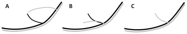
Effects of morphological features. A) Connecting the same dendritic points in different topologies has a large impact on charge transfer from synapse to soma, as shown by the varying responses (arrow size) to a stimulus in an identical location (lightning bolt). B) Branch centerlines determine path length and tortuosity, affecting signal propagation and providing clues about the underlying developmental processes. In terms of extrinsic determinants of branch growth, the left trace suggests a strong unidirectional signal (arrow) while the right trace reveals contributions from other directions. C) Precise tracing of dendrites and axons is important for determining potential connectivity. The left traces show a dendrite (black) and axon (gray) overlapping (arrowhead), while the right traces have no potential synapse due to the failure of the dendrite to extend all the way to the axon. Terminal nodes are all marked with a ‘T’.
Scientists planning large-scale projects are crucially interested in the amount of their time an algorithm will save in producing quality reconstructions. While future algorithms may be even better and more consistent than humans at reconstructing neurons, the current state of the art requires checking and editing automatically produced reconstructions (Luisi et al., 2011; Peng et al., 2011). Thus, different scientists might disagree as to the most suitable criteria to decide on whether an algorithm suits their needs.
Human subjectivity in the tracing process presents a challenge to measuring reconstruction quality, particularly given the challenges associated with staining and imaging (Jaeger, 2001). Resolution limits of current imaging methods make it sometimes impossible to ascertain correct connectivity. Histological limitations such as tissue shrinkage, physical sectioning of trees, and labeling gaps and artifacts provide further demands on reconstruction methods (Brown et al, 2011), and are important to consider when analyzing morphological data (Kaspirzhny et al., 2002). Methodological optimization and standardization of procedures, guided by collaboration between biologists and computer scientists, might reduce or eliminate such uncertainty by producing cleaner data. Until then, the metric design can reduce the effect of subjectivity by decreasing the weight of tree nodes (i.e. bifurcations and terminations) in more subjective zones, such as thin branches or distal locations, relative to the nodes in less subjective zones.
Many measures are commonly employed to analyze neuronal morphology, and new metrics continue to be introduced to capture specific features of dendritic and axonal arbors (e.g. Brown et al., 2008). However, most studies tend to compare groups of neurons under differing experimental conditions. The typical design tests whether a sample of neurons from treated animals significantly differs from a sample (of the same cell type) from controls in terms of one or more morphometrics (e.g. number of branches or total length). These classical morphological studies are complementary to the problem of comparing individual instances of the same neuron. The question of how to measure the quality of a reconstruction relative to a gold standard is instead similar to the issue of quantifying changes in neuronal morphology over time or in response to some stimulus or treatment. In these cases, a metric that registers the tree structures and compares them node by node or branch by branch can provide greater detail and analytical power. Provided changes in morphological features are not so drastic as to change the neurite fundamentally and prevent proper registration, the detected changes could be attributed to particular segments of the neurite that appear, disappear, or change in some manner.
This paper presents a metric originally designed to measure reconstruction quality for the DIADEM Challenge (DIgital reconstruction of Axonal and DEndritic Morphology). The Challenge aimed to encourage development of automated algorithms with the goal of reducing human interaction time while still generating high quality data. The term “metric” is not used here in the strict mathematical sense, as the DIADEM metric produces a similarity value (on the scale of 0 to 1) rather than a distance value. Moreover, it is asymmetric (i.e. the score may depend on which reconstruction is considered the gold standard) and does not satisfy the triangle inequality. Although certain features in the original version of the metric were specialized for the competition, the current release (http://diademchallenge.org) expands the set of options and includes the source code for optimal suitability to a broader range of applications. After briefly reviewing prior efforts, we describe the DIADEM metric and examine its relationship with other components of the reconstruction quality judging process.
Previous Relevant Work
Although no metric exists specifically to measure change or error in neuronal morphology, several approaches have been developed to quantify features and reconstruction quality of tree-like structures for related purposes. One class of methods registers the same regions of interest and embedded trees in multiple medical images to each other given changes over time. These methods are commonly applied to human airways and vasculature, which are subject to elastic deformation due to effects such as breathing, blood flow, and surgery (Metzen et al., 2009). Registration is accomplished by matching nodes and/or branches in the arborization (Charnoz et al., 2005; Tschirren et al., 2005; Drechsler et al., 2010) or by aligning path centerlines (Bülow et al., 2006). These approaches ignore spatial position since they account for tissue deformation (Fig. 2). While these methods are broadly applicable to the goal of measuring morphological error and change, deformation is not an issue when comparing multiple reconstructions of the same neuron (see however Canty and De Paola, 2011). For this application, therefore, there is little reason not to incorporate relevant positional information in the desired metric.
Fig. 2.

Tree registration and tree edit distance (TED). Methods that register nodes on deformed trees will match the dashed branches (nodes e and f with e* and f*), since topologically they are equivalent. Methods that include centerline or path matching will not match those branches. TED matches trees by their nodes and therefore will produce a distance score of 0 (i.e. a similarity score of 1). If TED distinguished the two branches, the distance score would be 4, i.e. one for each node added and removed (e, f, e*, f*).
The tree edit distance (TED) counts the number of nodes (both internal and terminal) that must be added or removed from one tree in order to create the second tree (Zhang, 1996). This pairwise metric has been applied to neuron classification (Heumann and Wittum, 2009) and to investigate stereotypy of neuromuscular fiber connectomes (Lu et al., 2009). However, TED is not spatially specific, while node locations are important in detecting morphological error or change. For example, when measuring quality, the double mistake of an extra branch and a missing branch extending from the same parent branch would be ignored by TED (see also Gillette and Grefenstette, 2009). The analogous situation for morphological plasticity would be the growth of one branch simultaneous with the retraction of another (i.e. within the same time frame, see Fig. 2). Using an edit cost function (i.e., counting changes required to create perfect similarity between trees) for length differences would only capture part of the difference. A registration method accounting for position will avoid such a problem.
Metrics developed to assess or validate algorithmic reconstructions in earlier automation efforts are also clearly of interest. The choice of validation strategy depends on the scientific aim or the perceived challenge. Previous selections included branch- and tree-level morphometrics (i.e. diameter, length, surface area), centerline accuracy, proportion of a gold standard reconstructed, and simulated electrophysiological activity (Wearne et al., 2005; Tyrrell et al., 2007; Losavio et al., 2008; Rodriguez et al., 2009; Peng et al., 2010b). Simulations may be ideal to explore the impact of reconstruction quality on specific neuron functions. However, they are time-consuming and make limiting assumptions in terms of biophysical properties and stimulation protocols. Standard morphometrics suffer from the same issue described for TED, whereby a parameter such as overall surface area could stay constant while different parts of the tree are changing in opposite ways. Distributions of those metrics may be more informative, but complete specification of all changes throughout the neuron requires registration and analysis of all branches.
Description of the DIADEM Metric
In comparing two arbors, the DIADEM metric registers and scores each corresponding node and its parent branch individually on the basis of connectivity with the local region of the tree. A rigid registration of nodes is used in order to make use of positional information, which is intuitively sensible when dealing with two reconstructions of the same underlying image data. In the case of comparing the same neurite at different times, the amount of change would have to be small enough that an identifiable core object is shared between time points. Adjustments for tissue deformation due to slice preparation or microscope stage drift would be necessary preprocessing steps. Emphasis on topologically relevant features over diameter and centerline geometry is justified in part by the influence of branch topology on signal processing and its dependence on growth mechanisms (van Pelt et al., 1992; Ascoli, 2002; Koene et al., 2009). Though vital to understanding neuron function, diameter evaluation is highly subjective at resolutions used for full neuronal arbor reconstruction (Jaeger, 2001; Scorcioni et al., 2004), and was not considered in the DIADEM competition. Centerlines were deemed important in terms of reproducing distances along the neurite path. This aspect was incorporated in the metric without the need for continuous scoring of centerline quality. The metric input is specified in SWC format1, which represents trees by individual points in space with connections denoted by unique numerical identities. Below we explain the computational essence of the DIADEM metric. More extensive implementation details are provided in the online documentation and through distribution of the source code (http://diademchallenge.org/metric.html).
Each node in the “gold standard” arborization (e.g. the manual reconstruction) is taken as the ground truth and is registered to a node in the “test” arborization (e.g. the automated reconstruction). The process begins with the most proximal gold standard bifurcation, proceeds to the first bifurcation’s children, then to their children, and so on until registration has been attempted for all gold standard nodes. Registration requires the test nodes to be located spatially within a cylindrical threshold region around the gold standard node, as determined by the chosen data set or by user discretion. This represents the region in which one might reasonably create a bifurcation or termination in the trace given subjectivity and resolution in the XY plane and Z axis (Fig. 3A,B). As either gold standard or test node could be at an edge of a bifurcation or termination, the radius of the threshold region was chosen to be the diameter of one of the larger bifurcations within each of the data sets used in the DIADEM competition in order to accommodate the more extreme (but still reasonable) cases. Image resolution, staining contrast, and depth of focus all influenced threshold choices such that sufficiently low resolution or contrast could result in larger thresholds if the neurite edges were less clear in the XY plane or Z-axis. Registered nodes are expected to have matching paths to matching ancestor nodes (i.e. bifurcation nodes between the nodes of interest and the tree roots). Ancestor node matches are found by traversing toward the tree root from the gold standard node and from the potentially matching test node until the current ancestors of either tree are within the Euclidean distance threshold of each other (Fig. 3C). The traversal takes place on one tree at a time, on the tree with the shortest path from the current ancestor back to its respective node of interest. Once an ancestor match is found, the path test is performed and the potential match is either confirmed or discarded.
Fig. 3.

The DIADEM metric. A) The filled central circle intersected by the branches is the bifurcation node. The cylinder represents the 3D threshold region, within which potential matches may be located. The cylinder is generated from expanding the XY threshold circle to the bounds of the Z threshold. B) A trace could validly bifurcate anywhere within the specified region (single white ring). Here the gold standard (solid trace) bifurcates at the edge of the region. To account for the lack of information on the location of the neurite centerline, the threshold region (double white ring) has a radius twice that of the valid region. Thus a test trace (dashed) that bifurcates at the opposite edge will still be matched. C) Establishing branch connectivity with an ancestor. The target node of the gold standard reconstruction (double ring) has a candidate test node in both test trees to the right. The × symbols are the ancestors of the target node that have no match in Test Tree A, and the ancestors of the potential match in Test Tree A that have no match in the gold standard. However, the black ring ancestor matches spatially and in terms of path to target, resulting in a hit for Test Tree A. Test Tree B has an ancestor in the right location, but the length of its path to the target node is incorrect (dashed ring), resulting in a miss for Test Tree B.
To determine whether the gold standard and test paths match, an acceptable test path must have a sufficiently small error along a given component (i.e. on the XY plane or the Z axis) relative to the full three-dimensional path length. This “path length error” is calculated as the difference between the gold standard and candidate test path length in a given component, divided by the full gold standard path length. This method is one source of asymmetry in the metric. Another is the method for adjusting the test path length to account for differences in position of the ancestor and descendant from their respective gold standard matches (described in greater detail on the DIADEM Challenge website). Acceptable path length error is given by a second pair of thresholds, which for the DIADEM data sets were determined based on the straightest possible path and the longest reasonable path that stayed within the bounds of the neurite. Users may set their own path length error thresholds. A very large threshold might be chosen if path length is anticipated to be unreliable and unimportant in terms of data usage. If multiple test nodes are suitable for registration to a given gold standard node based on the criteria above, the one with a descendant and path to the descendant that matches a descendant (and path) of the gold standard node is registered. If there are still multiple candidates or no candidates exhibit matching descendant connectivity, the test node spatially closest is registered.
Once registration has been attempted for all gold standard nodes, those nodes that fail to be registered to a test node are each considered a second time to determine whether the test tree at least captures the path through the location of the gold standard node. This situation can occur when there is a bifurcation in the gold standard but only one of the two child branches is traced in the test reconstruction resulting in a single path with no bifurcation node to use for registration. Without accounting for these cases, test reconstructions would be counted as having missed the path leading up to the gold standard bifurcation node even though it was traced (Fig. 4). The matching path is found by first traversing the gold standard reconstruction toward the root. When an ancestor that has been registered to a test node is found, the gold standard tree is then traversed from the target gold standard node toward its terminal ends. If no test descendent nodes match the path between this matched ancestor and the two gold standard descendants, paths to nodes further downstream are checked for matches. The number of descendant paths followed depends on the number of downstream bifurcations, but the traversal of any given path ends when a descendant is encountered that is registered to a test node. The same criteria for node matching described above applies here for matching descendents, including having similar path lengths to the ancestor of the gold standard node in question. The process is continued until a path match is found, or until all potential descendant paths are exhausted. If a matching path is found, the test tree is scored as having a match to the gold standard node since the test path is deemed to have captured the same path up to the node location on the gold standard node. The absence of the second branch is penalized in the initial registration process by the lack of a match of its terminal node (or subtree).
Fig. 4.

Matching paths through unregistered nodes. Symbols on the gold standard correspond with symbols on Test Tree A, which has a matching path (thick path) for the unregistered gold standard node of interest (double ring). Test Tree B results in a miss for the gold standard node and path. The × symbols mark an ancestor and two descendants without matches in either test tree. Both test trees do contain a matching ancestor (ring above target). Several descendants have potential matches (dashed rings and their descendants), but fail to produce matching paths to the ancestor. The position of the second descendant (solid single ring below target) and its path to the ancestor do match in Test Tree A. No descendants in Test Tree B match by path, and thus Test Tree B does not contain a matching path for the gold standard target node.
Several alternative options provide greater flexibility depending on the intended use of the metric. Nodes can be weighed differentially, for instance by degree (i.e. number of terminal nodes in the sub-tree) in order to capture topologically important bifurcations, or uniformly if terminal nodes are as relevant to the user. In the DIADEM competition, nodes were weighed by degree primarily due to the larger functional impact of larger sub-trees. In several of the DIADEM gold standards, tracing subjectivity was also particularly high in terminal regions, with more frequent branching and neurite overlap (Brown et al., 2011). Thus, this weighing scheme also reduced the contribution of the more subjective regions to the score. Another choice is whether to tally as misses the excess nodes in the test reconstruction that are not in the gold standard. Rules are in place to prevent non-matched test nodes that appear to be reasonable attempts (i.e. the bifurcation or termination is close to a gold standard node) from counting as excess nodes (Fig. 5). The miss in the gold standard in these cases is considered to be a sufficient penalty to the score. If used for measuring changes in neurite morphology, a suitable alternative could be to consider all unmatched test nodes as new branches by counting them all as excess nodes rather than using any criteria to excuse them. Lastly, terminal test nodes that terminate in the wrong location can be scored as matches if their path is approximately correct. While not part of the default mode, this option was used in order to prevent penalizing automated algorithms that traced rosette structures in the neuromuscular projection fiber data set (Fig. 6). Further potential uses of this option are discussed later. In applying the DIADEM metric, the weighing scheme and other parameters must be determined based on a combination of goals, including minimizing subjectivity and maximizing functionally relevant features.
Fig. 5.
Determining excess nodes. A) The terminal node of the gold standard (black) is a miss due to its incorrect path. The gray test termination is not an excess node because there is a gold standard node within threshold distance. Since the termination does not count as an excess node, the parent bifurcation is not counted against the score either. B) The gold standard terminal node is a miss due to the incorrect position of the test terminal (gray). However, the test termination is not an excess node since its parent bifurcation is matched. C) The gray test termination has no basis in the gold standard reconstruction and so it is an excess node.
Fig. 6.
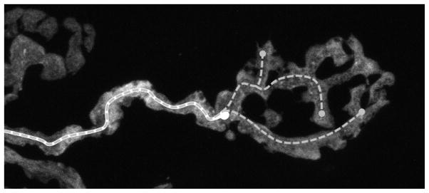
Neuromuscular projection axon rosette. The gold standard (solid white trace, which overlaps with the dashed gray line) tracks the path of the axon until it ends at the beginning of the rosette structure. The test reconstruction (dashed gray) follows the same path yet continues into the rosette, and will still be successfully matched. This approach could also be used for measuring the growth of a neurite captured across multiple reconstructions in a time series.
Human Expert Qualitative Scores and Interaction Time
In alternative or addition to an objective metric, the quality of a reconstruction can be evaluated directly by a domain expert. After the Qualifier Round of the DIADEM Challenge (Brown et al., 2011), several experienced neuroscientists judged the quality of the submitted reconstructions. All judges were principal investigators of laboratories that had produced several peer-reviewed publications using neuronal reconstructions. Although no strict constraints were mandated as to how to score submissions, guidelines were provided in terms of the possible reconstruction errors that should be looked for. These included missing a large sub-tree, missing small branches, tracing non-existing or unconnected trees, tracing extra small branches, incorrectly positioning bifurcations and terminations, incorrectly connecting branches and trees, incorrectly tracing a segment path, and tracing a segment in the wrong direction. The judges determined for themselves how to weigh each type of error. Their scores ranged from 0 to 10, but were rescaled 0 to 1 for comparison purposes with other metrics. In the analysis these scores are referred to as “qualitative scores”. “Average qualitative score” will refer to the average of scores from multiple judges for one automated reconstruction.
Reconstruction algorithms cannot yet consistently produce reconstructions of gold standard quality. Nevertheless, their output may be of sufficient quality such that editing it could take considerably less time than reconstructing the same neuron from scratch. Thus, the effectiveness of an automated reconstruction algorithm can also be measured by an expert determination of the amount of time saved compared to a manual process (Chklovskii et al., 2010). A person highly experienced in reconstructing a neuron from a particular preparation can produce an accurate estimate by clocking the interaction time taken to reconstruct a neurite sample from scratch. Then, the same operator clocks the time necessary to edit the reconstruction of an equivalent sample produced by the automated algorithm until it is of the same quality as that generated manually. The resulting score, hereto referred to as the “interaction time score” or simply “interaction score”, would be specific to the type of data and may contain some subjectivity reflecting the individual’s strengths and weaknesses in terms of speed in reconstructing or editing specific morphological features. However, the score directly addresses the scientist’s main concern by quantifying the time saved by the evaluated algorithm.
Submissions of the DIADEM Qualifier Round were scored according to this criterion in addition to applying the DIADEM metric and the expert qualitative assessment. In particular, the owners of the data sets used in the competition scored the entries by determining how long it would take to edit them up to gold standard quality without simultaneously viewing the gold standard. Experience with a particular image stack could lead to a decrease in editing time for a data owner independently of reconstruction quality. In order to minimize the relative improvement between reconstructions from different teams of the same neuron, the data owners were instructed to start by scoring the manual reconstruction. Data set owners also shuffled the order in which team reconstructions were edited. While this second factor reduced bias toward any team, it would not eliminate the experience effect on scores for the analysis comparing the interaction time and the metric. Data set owners only scored reconstructions of their own neurons, and in many cases only scored a subset of those. For any submission that was edited, the judge either reconstructed the section or estimated the amount of time it would take to do so, but in either case was consistent in their practice. The corresponding score for a given reconstruction was one minus the ratio between the amount of time needed to edit the reconstruction and the total time taken to manually reconstruct the same structure. Thus a score of zero would correspond to no time savings, and a score of one would correspond to a perfect automated reconstruction requiring no editing time.
Utility of the DIADEM Metric
In order to determine whether the DIADEM metric is useful for evaluating reconstruction quality, it is important to compare it to expert judgments. Indeed, comparison between the various scoring methods showed strong correlations, suggesting that the metric may be viable as a machine-derived surrogate to human judging (Fig. 7). Specifically, the correlation across reconstructions between the metric and the qualitative score averaged from four different judges was R = 0.66 (p < 10−5). Correlation between the metric and interaction time scores was R = 0.77 (p < 10−6) when controlling for judge and data set. All correlations with interaction time scores are determined using a linear model of interaction time score as the dependent variable, and the correlate (in this case the metric score) and data set as the independent variables, without any interaction effects. The R value is derived from the resulting adjusted R2 of the model. This normalization step is necessary because, while each qualitative judge scored every data set, each data owner only clocked the interaction time for their own data set. Thus interaction times could be affected both by the judge’s methods and data specific features, as confirmed by the statistically non-significant correlation of R = 0.09 (p = 0.6) in the absence of control.
Fig. 7.

The gold standard and automated reconstructions (T1–T3) of a hippocampal CA3 interneuron dendrite submitted in the Qualifier Round of the DIADEM Challenge. The qualitative score, interaction time, and DIADEM metric for each reconstruction exemplify how various errors can impact different scoring methods. On this small tree, T1 received a low DIADEM metric score due to unsmoothed paths which inflated path length (zoom box) causing path length error to surpass the threshold. A smoothed path or more lenient path length threshold would result in a higher score more consistent with human expert judgment which ignores the effect of the jagged path. In T3, too many excess nodes resulted in low scores for all measures.
If the data set effect is in fact a judge effect, then the metric can better serve as a comparison than interaction time scores produced by different judges (at different labs). However, variability in interaction time scores could be due to tree size, which varies substantially among data sets (Table 1). If tree size explained the score variability, a model of metric and interaction time including tree size should show a strong tree size effect and a correlation similar to that observed in the model that included data set as a parameter. Instead, such a model produced a poorer correlation. Moreover, a model including both data set and tree size showed no significant effect of tree size. Therefore, while tree size may have some effect on scores, it is clearly not responsible for variation in interaction times between data sets. Further evidence in this regard comes from the variability in qualitative judge scores. The four qualitative scores for each of the selected reconstruction submissions had an average range of 0.3 and an average standard deviation of 0.14. While experts may each be consistent in their judgments, these results suggest that an objective measure such as the DIADEM metric will better serve for comparing reconstruction qualities across studies.
Table 1.
Scores across data sets. Values are means ± standard deviations. Tree size refers to the number of branches of the gold standard reconstructions. The Climbing Fiber data set had only one gold standard reconstruction, thus it has no standard deviation. The “Uniform” column represents values from the DIADEM metric with nodes weighed uniformly.
| Data set | Tree Size | Qualitative | Interaction | DIADEM | Uniform |
|---|---|---|---|---|---|
| Climbing Fiber (n=5) | 199 | 0.46 ± 0.27 | 0.11 ± 0.18 | 0.37 ± 0.28 | 0.22 ± 0.16 |
| Hippocampal CA3 (n=14) | 4 ± 2.2 | 0.58 ± 0.26 | 0.66 ± 0.16 | 0.39 ± 0.32 | 0.44 ± 0.31 |
| Neocortical (n=13) | 8.2 ± 7.5 | 0.4 ± 0.17 | 0.41 ± 0.17 | 0.28 ± 0.3 | 0.25 ± 0.27 |
| Olfactory Projection (n=8) | 26 ± 9.6 | 0.8 ± 0.06 | 0.3 ± 0.15 | 0.78 ± 0.1 | 0.58 ± 0.09 |
The correlation between the DIADEM metric and either of the other two methods (qualitative evaluation and interaction time) is nearly as strong as the correlation between the two human scores, indicating that the metric might capture fundamental features shared by expert judgment. Again controlling for data set, the correlation between qualitative scores and interaction time was R = 0.83 (p < 10−8). A linear model controlling for data set also confirms the data set effect in the interaction scores. For example, the hippocampal CA3 interneuron (p < 10−7) and neocortical layer 6 axon (p < 10−4) data sets had significant effects when the cerebellar climbing fiber data set is taken as the base model (Fig. 8). This was the same pattern observed in the model of DIADEM metric and interaction time scores. While each measure of reconstruction quality (relative to a gold standard) is unique, the analysis suggests that the measures all are strongly related to each other and that the DIADEM metric can serve as a surrogate for expert qualitative and interaction time judgment (see Table 2 for summary of correlations).
Fig. 8.

Relationships between scoring methods. Data sets are identified with different symbols and abbreviations (HC: hippocampal CA3 interneuron; OP: olfactory projection fibers; NC: neocortical layer 6 axons; CF: cerebellar climbing fibers). All scores were normalized to a scale of 0 (incorrect) to 1 (perfect). A) Separation of scores by data set clearly shows the effect of data set on interaction times. B) The lower DIADEM metric scores (along the left edge) are responsible for much of the lack of correlation. These scores are largely due to terminal branches that track the gold standard well, but terminate in the wrong location. The effect is much stronger in the data sets containing trees with fewer branches (HC and NC).
Table 2.
Summary of correlations. All correlations are highly significant (p < 0.001). Values mirrored over the diagonal for ease of comparison.
| DIADEM Metric | Qualitative | Interaction Time | TED | |
|---|---|---|---|---|
| DIADEM Metric | 0.66 | 0.77 | 0.52 | |
| Qualitative | 0.66 | 0.83 | 0.54 | |
| Interaction Time | 0.77 | 0.83 | 0.75 | |
| TED | 0.52 | 0.54 | 0.75 |
Note: Values are Pearson correlation coefficients, except for those associated with Interaction Time (gray background), which are each calculated as the square root of the adjusted R2 of the linear model. The models take Interaction Time as a function of data set and a specific scoring method.
The effects of specific scoring method differences are more difficult to tease apart. Some of the remaining variance could in principle be attributed to the factors that are differentially weighed in each scoring system. For instance, while the DIADEM metric weighs nodes by terminal degree, the interaction time score does not necessarily differentiate nodes by sub-tree size. However, a variant of the metric with uniform weights produced no better correlation with interaction time scores (R = 0.75) or qualitative scores (R = 0.63). As an alternative explanation, judges might not necessarily mark a branch as incorrect just because it terminates too early or too late, thus differing from the DIADEM metric (Fig. 8B). Another source of variance that could not be controlled for was the increased experience of interaction time judges over a set of reconstructions of the same underlying neurite. Shuffling the order across team reconstructions alleviates bias for or against teams, but it is still possible that two reconstructions of the same neurite and of equal quality could receive different interaction time scores. Despite these sources of variance and other unexplained sources, the correlation results suggest that the DIADEM metric can serve as a complementary judgment of features that are more difficult to visualize, particularly branch topology (Fig. 9). Different connectivities within two complex trees can have a profound effect on signal propagation and/or integration, even if spatially similar and thus easily missed by the human eye.
Fig. 9.

Selected region of cerebellar climbing fiber single slice with gold standard overlay (left) and sample automated reconstruction overlay (right). While some errors in the automated reconstruction are more obvious, the mistake in the central region is more difficult to discern without close attention. The right side of the gold standard trace runs from a bifurcation near the bottom to the top, but the automated reconstruction creates a non-existent bifurcation which leads the trace downward and stops, yielding an excess terminal node (arrowhead). While the bottom bifurcation (bifurcating white arrows) is seen as a continuation, the error produces another missed bifurcation immediately above it (hollow circle) and then an additional two missed terminations.
The importance of positional information is demonstrated by comparing the DIADEM metric to the tree edit distance (TED) described above (Heumann and Wittum, 2009). In order to compare the two measures, tree edit distances values were normalized by the gold standard tree size and inverted in order to generate comparable similarity values. TED correlations with qualitative scores (R = 0.54) and with interaction times (R = 0.75) were lower than those of the DIADEM metric. The correlation between TED and the DIADEM metric improved from 0.52 to 0.68 when considering only gold standard reconstructions with degree greater than 3 (more than 5 branches). This change, and much of the lower correlation, could be due to the fact that two trees could have the exact same topology yet differ in terms of branch locations. This is a substantial risk particularly for small trees with few distinct topologies. The higher DIADEM scores may reflect the treatment of continuations as hits, where cost is calculated at the missing descendents, as TED tallies continuations as deleted nodes, and each extra branch as two added nodes. Recognizing continuations as hits is important as the node also represents its parent branch. Thus, the DIADEM metric is more appropriate than TED for the task of measuring reconstruction quality or morphological change of a neuron.
Discussion
The DIADEM metric was designed to quantify the differences between two reconstructions of the same neuron. Its ability to provide useful scores of reconstruction quality was confirmed by strong correlations with expert qualitative judgments and measures of interaction time required to fix reconstruction errors. Thus, the DIADEM metric could greatly aid the development and tuning process of automated reconstruction algorithms. The metric also has particular qualities that would make it useful for measuring morphological change of a neuron over time due to development, plasticity, or other experimental factors.
The DIADEM metric is released open source to encourage future implementation of further improvements. A more sophisticated path matching module would decrease the likelihood of false positives (incorrectly registering nodes) while creating an option to score a node based on its parent branch centerline quality. An average distance method used on vasculature centerlines (Schaap et al., 2009) could be adapted to the DIADEM metric, given the known starting and ending locations of the path. Such an approach would match points along both reconstruction paths, then find the average distance between paths. Alternatively, a sequence alignment method using position and curvature (direction) could also increase path matching accuracy (Cardona et al., 2010). This method would be particularly useful in cases of deformation where a larger position threshold is required and a simple average distance is insufficient.
While a direct comparison of the DIADEM metric with the basic TED showed the metric to better represent expert judgment, the potential of TED is worth consideration for use in a future improved metric. Heumann and Wittum (2009) tested a variety of node labels, evaluating matched nodes and assigning some cost to differences in matched node properties. A variant TED might be designed that uses node position as part of a node label, and using a nonlinear node edit distance function that evaluates to 0 within a threshold range, and to infinity beyond that range. This would at least handle the issue of node position, one of the primary characteristics of the DIADEM metric. Such a scheme would also allow inclusion of other branch features such as path length or surface area. This would be even more useful in measuring morphological change. Enabling non-binary scoring for each node based on branch features would create options particularly suited to measuring differences in a neuron over time, such as terminal retraction or elongation. Nevertheless, these variations on the TED alone would still fall short of the DIADEM metric functionality. An advanced DIADEM inspired metric might incorporate those aspects of the TED into an algorithm that also weighs nodes, handles continuations, and makes allowances for certain unmatched test nodes (i.e. excess node testing). Moreover, in order to capture qualitative judgment of terminal nodes that are too long or too short (or to properly measure growth or retraction of terminal nodes), terminal node matching would require specialized processing such as that applied in the neuromuscular projection fiber rosette case (Fig. 7). Thus, although appropriate TED variations might approach the capabilities of the DIADEM metric, only in merging the two approaches would its benefits be fully realized.
Repeated gold standards are invaluable to account for subjectivity in evaluating reconstructions. A method for measuring the quality of algorithms to reconstruct arterial centerlines used a reference composed of several manual reconstructions produced by different people (Schaap et al., 2009). While averaged centerlines (and their variances) can be used to evaluate paths between nodes, the topology of trees cannot be averaged since the paths between nodes either do or do not exist. However, if multiple gold standard reconstructions are available, a test reconstruction node and its path could be considered valid if matches were present in a representative sample of the gold standards. Overall, an automated algorithm should be deemed of “gold standard quality” if its product falls within the variability displayed by the manual reconstructions generated by several independent experts. A more detailed analysis would be required for any data set to determine how many manual reconstructions are needed to capture the full range of subjectivity.
A metric that tests automated reconstructions can also serve in an iterative process of improving the algorithm or tuning its parameters. While developers may choose to use it as a separate step, the DIADEM metric can also be integrated into a development pipeline that automatically searches optimal parameters for a given data type. The metric can return missed nodes, nodes marked as continuations, and excess nodes. It could further be enabled to output other details such as centerline precision. Such information could aid identification of the most challenging features for the reconstruction algorithm, as well as tracking of the changes that produce improvements for specific node types.
In conclusion, assuming a manual reconstruction is available to use as the gold standard, the DIADEM metric captures a substantial proportion of expert qualitative judgment and editing time, and it can also detect topological errors easily missed by humans. Future implementations utilizing the ability of the metric to register topology and measure node-specific differences will enhance its potential to also quantify neuromorphological change in time.
Acknowledgments
We are grateful to Dr. Karel Svoboda for early discussions on the development of the DIADEM metric. This work was supported in part by HHMI and NIH grant R01NS39600.
Footnotes
Information Sharing Statement: The DIADEM metric executable is a cross-platform JAR file which can be run by the Java Virtual Machine on any computer or operating system. The executable, code, documentation, and instructions for use are available at http://diademchallenge.org.
References
- Ascoli GA. Neuroanatomical algorithms for dendritic modelling. Network. 2002;13:247–260. [PubMed] [Google Scholar]
- Ascoli GA, Alonso-Nanclares L, Anderson SA, Barrionuevo G, Benavides-Piccione R, Burkhalter A, et al. Petilla terminology: nomenclature of features of GABAergic interneurons of the cerebral cortex. Nature Reviews Neuroscience. 2008;9:557–568. doi: 10.1038/nrn2402. [DOI] [PMC free article] [PubMed] [Google Scholar]
- Baloyannis SJ. Dendritic pathology in Alzheimer’s disease. Journal of the Neurological Sciences. 2009;283:153–157. doi: 10.1016/j.jns.2009.02.370. [DOI] [PubMed] [Google Scholar]
- Binzegger T, Douglas RJ, Martin KA. A quantitative map of the circuit of cat primary visual cortex. Journal of Neuroscience. 2004;24:8441–8453. doi: 10.1523/JNEUROSCI.1400-04.2004. [DOI] [PMC free article] [PubMed] [Google Scholar]
- Brown KM, Donohue DE, D’Alessandro G, Ascoli GA. A cross-platform freeware tool for digital reconstruction of neuronal arborizations from image stacks. Neuroinformatics. 2005;3:343–359. doi: 10.1385/NI:3:4:343. [DOI] [PubMed] [Google Scholar]
- Brown KM, Gillette TA, Ascoli GA. Quantifying neuronal size: summing up trees and splitting the branch difference. Seminars in Cell & Developmental Biology. 2008;19:485–493. doi: 10.1016/j.semcdb.2008.08.005. [DOI] [PMC free article] [PubMed] [Google Scholar]
- Brown KM, Barrionuevo G, Canty AJ, De Paola V, Hirsch JA, Jefferis GSXE, et al. The DIADEM data sets: representative light microscopy images of neuronal morphology to advance automation of digital reconstructions. Neuroinformatics. 2011 doi: 10.1007/s12021-010-9095-5. this issue. [DOI] [PMC free article] [PubMed] [Google Scholar]
- Bülow T, Lorenz C, Wiemker R, Honko J. Point based methods for automatic bronchial tree matching and labeling. Proceedings of the SPIE. 2006;7:225–234. [Google Scholar]
- Canty AJ, De Paola V. Axonal reconstructions going live. Neuroinformatics. 2011 doi: 10.1007/s12021-011-9112-3. this issue. [DOI] [PMC free article] [PubMed] [Google Scholar]
- Capowski JJ. An automated neuron reconstruction system. Journal of Neuroscience Methods. 1983;8:353–364. doi: 10.1016/0165-0270(83)90092-4. [DOI] [PubMed] [Google Scholar]
- Cardona A, Saalfeld S, Arganda I, Pereanu W, Schindelin J, Hartenstein V. Identifying neuronal lineages of Drosophila by sequence analysis of axon tracts. Journal of Neuroscience. 2010;30:7538–7553. doi: 10.1523/JNEUROSCI.0186-10.2010. [DOI] [PMC free article] [PubMed] [Google Scholar]
- Charnoz A, Agnus V, Malandain G, Soler L, Tajine M. Tree matching applied to vascular system. In: Brun L, Vento M, editors. Graph-Based Representations in Pattern Recognition. Springer; Berlin, Heidelberg: 2005. pp. 183–192. [Google Scholar]
- Chklovskii DB, Vitaladevuni S, Scheffer LK. Semi-automated reconstruction of neural circuits using electron microscopy. Current Opinion in Neurobiology. 2010;20:667–675. doi: 10.1016/j.conb.2010.08.002. [DOI] [PubMed] [Google Scholar]
- Cline H. Dendritic arbor development and synaptogenesis. Current Opinion in Neurobiology. 2001;11:118–126. doi: 10.1016/s0959-4388(00)00182-3. [DOI] [PubMed] [Google Scholar]
- Cuntz H, Forstner F, Borst A, Häusser M. The TREES Toolbox – Probing the Basis of Axonal and Dendritic Branching. Neuroinformatics. 2011 doi: 10.1007/s12021-010-9093-7. in press. [DOI] [PMC free article] [PubMed] [Google Scholar]
- Drechsler K, Laura CO, Chen Y, Erdt M. Semi-automatic anatomical tree matching for landmark-based elastic registration of liver volumes. Journal of Healthcare Engineering. 2010;1:101–124. [Google Scholar]
- Gillette TA, Grefenstette JJ. On comparing neuronal morphologies with the constrained tree-edit-distance. Neuroinformatics. 2009;7:191–194. doi: 10.1007/s12021-009-9053-2. [DOI] [PubMed] [Google Scholar]
- Glaser EM, Van der Loos H. A semi-automatic computer microscope for the analysis of neuronal morphology. IEEE Transactions on Biomedical Engineering. 1965;12:22–40. [PubMed] [Google Scholar]
- Glaser JR, Glaser EM. Neuron imaging with Neurolucida – a PC-based system for image combining microscopy. Computerized Medical Imaging and Graphics. 1990;14:307–317. doi: 10.1016/0895-6111(90)90105-k. [DOI] [PubMed] [Google Scholar]
- Goldberg J, Hamzei-Sichani F, MacLean J, Tamas G, Urban R, Yuste R. From dendrites to networks: optically probing the living brain slice and using principal component analysis to characterize neuronal morphology. In: Zaborszky L, Wouterlood FG, Lanciego JL, editors. Neuroanatomical Tract-Tracing 3: Molecules, Neurons, and Systems. Springer; US: 2006. pp. 452–476. [Google Scholar]
- Hao H, Shreiber DI. Axon kinematics change during growth and development. Journal of Biomechanical Engineering. 2007;129:511–522. doi: 10.1115/1.2746372. [DOI] [PubMed] [Google Scholar]
- Haug H. Brain sizes, surfaces, and neuronal sizes of the cortex cerebri: A stereological investigation of man and his variability and a comparison with some mammals (primates, whales, marsupials, insectivores, and one elephant) American Journal of Anatomy. 1987;180:126–142. doi: 10.1002/aja.1001800203. [DOI] [PubMed] [Google Scholar]
- Heumann H, Wittum G. The Tree-Edit-Distance, a measure for quantifying neuronal morphology. Neuroinformatics. 2009;7:179–190. doi: 10.1007/s12021-009-9051-4. [DOI] [PubMed] [Google Scholar]
- Jaeger D. Accurate reconstruction of neuronal morphology. In: de Schutter E, editor. Computational Neuroscience: Realistic Modeling for Experimentalists. CRC Press; 2001. pp. 159–178. [Google Scholar]
- Kaspirzhny AV, Gogan P, Horcholle-Bossavit G, Tyc-Dumont S. Neuronal morphology data bases: morphological noise and assesment of data quality. Network. 2002;13:357–380. [PubMed] [Google Scholar]
- Kasthuri N, Lichtman JW. Neurocartography. Neuropsychopharmacology. 2010;35:342–343. doi: 10.1038/npp.2009.138. [DOI] [PMC free article] [PubMed] [Google Scholar]
- Koene RA, Tijms B, van Hees P, Postma F, de Ridder A, Ramakers GJ, et al. NETMORPH: a framework for the stochastic generation of large scale neuronal networks with realistic neuron morphologies. Neuroinformatics. 2009;7:195–210. doi: 10.1007/s12021-009-9052-3. [DOI] [PubMed] [Google Scholar]
- Krichmar JL, Nasuto SJ, Scorcioni R, Washington SD, Ascoli GA. Effects of dendritic morphology on CA3 pyramidal cell electrophysiology: a simulation study. Brain Research. 2002;941:11–28. doi: 10.1016/s0006-8993(02)02488-5. [DOI] [PubMed] [Google Scholar]
- Li Y, Brewer D, Burke RE, Ascoli GA. Developmental changes in spinal motoneuron dendrites in neonatal mice. Journal of Comparative Neurology. 2005;483:304–317. doi: 10.1002/cne.20438. [DOI] [PubMed] [Google Scholar]
- Lin B, Masland RH. Synaptic contacts between an identified type of ON cone bipolar cell and ganglion cells in the mouse retina. The European Journal of Neuroscience. 2005;21:1257–1270. doi: 10.1111/j.1460-9568.2005.03967.x. [DOI] [PubMed] [Google Scholar]
- Losavio BE, Liang Y, Santamaría-Pang A, Kakadiaris IA, Colbert CM, Saggau P. Live neuron morphology automatically reconstructed from multiphoton and confocal imaging data. Journal of Neurophysiology. 2008;100:2422–2429. doi: 10.1152/jn.90627.2008. [DOI] [PubMed] [Google Scholar]
- Lu J, Tapia J, White O, Lichtman J. The Interscutularis Muscle Connectome. PLoS Biology. 2009;7:265–277. doi: 10.1371/journal.pbio.1000032. [DOI] [PMC free article] [PubMed] [Google Scholar]
- Luisi J, Narayanaswamy A, Galbreath Z, Roysam B. The FARSIGHT Trace Editor. Neuroinformatics. 2011 doi: 10.1007/s12021-011-9115-0. this issue. [DOI] [PubMed] [Google Scholar]
- Mainen Z, Sejnowski T. Influence of dendritic structure on firing pattern in model neocortical neurons. Nature. 1996;382:363–366. doi: 10.1038/382363a0. [DOI] [PubMed] [Google Scholar]
- Markram H, Toledo-Rodriguez M, Wang Y, Gupta A, Silberberg G, Wu C. Interneurons of the neocortical inhibitory system. Nature Reviews Neuroscience. 2004;(5):793–807. doi: 10.1038/nrn1519. [DOI] [PubMed] [Google Scholar]
- Marks WB, Burke RE. Simulation of motoneuron morphology in three dimensions. I. Building individual dendritic trees. The Journal of Comparative Neurology. 2007;503:685–700. doi: 10.1002/cne.21418. [DOI] [PubMed] [Google Scholar]
- Metzen JH, Kröger T, Schenk A, Zidowitz S, Peitgen H, Jiang X. Matching of anatomical tree structures for registration of medical images. Image and Vision Computing. 2009;27:923–933. [Google Scholar]
- Meyer-Luehmann M, Spires-Jones TL, Prada C, Garcia-Alloza M, de Calignon A, Rozkalne A, et al. Rapid appearance and local toxicity of amyloid-beta plaques in a mouse model of Alzheimer’s disease. Nature. 2008;451:720–724. doi: 10.1038/nature06616. [DOI] [PMC free article] [PubMed] [Google Scholar]
- Mize RR. Computer applications in cell and neurobiology: a review. International Review of Cytology. 1984;90:83–124. doi: 10.1016/s0074-7696(08)61488-6. [DOI] [PubMed] [Google Scholar]
- Overdijk J, Uylings HBM, Kuypers K, Kamstra AW. An economical semi-automatic system for measuring cellular tree structures in three dimensions, with special emphasis on Golgi-impregnated neurons. Journal of Microscopy. 1978;114:271–284. doi: 10.1111/j.1365-2818.1978.tb00137.x. [DOI] [PubMed] [Google Scholar]
- Peng H, Ruan Z, Long F, Simpson JH, Myers EW. V3D enables real-time 3D visualization and quantitative analysis of large-scale biological image data sets. Nature Biotechnology. 2010a;28:348–353. doi: 10.1038/nbt.1612. [DOI] [PMC free article] [PubMed] [Google Scholar]
- Peng H, Ruan Z, Atasoy D, Sternson S. Automatic reconstruction of 3D neuron structures using a graph-augmented deformable model. Bioinformatics. 2010b;26:i38–i46. doi: 10.1093/bioinformatics/btq212. [DOI] [PMC free article] [PubMed] [Google Scholar]
- Peng H, Long F, Zhao T, Myers E. Proof-editing is the bottleneck of 3D neuron reconstruction: the problem and solutions. Neuroinformatics. 2011 doi: 10.1007/s12021-010-9090-x. this issue. [DOI] [PubMed] [Google Scholar]
- Rodriguez A, Ehlenberger DB, Hof PR, Wearne SL. Three-dimensional neuron tracing by voxel scooping. Journal of Neuroscience Methods. 2009;184:169–175. doi: 10.1016/j.jneumeth.2009.07.021. [DOI] [PMC free article] [PubMed] [Google Scholar]
- Schaap M, Metz CT, van Walsum T, van Der Giessen AG, Weustink AC, Mollet NR, et al. Standardized evaluation methodology and reference database for evaluating coronary artery centerline extraction algorithms. Medical Image Analysis. 2009;13:701–714. doi: 10.1016/j.media.2009.06.003. [DOI] [PMC free article] [PubMed] [Google Scholar]
- Schaefer AT, Larkum ME, Sakmann B, Roth A. Coincidence detection in pyramidal neurons is tuned by their dendritic branching pattern. Journal of Neurophysiology. 2003;89:3143–3154. doi: 10.1152/jn.00046.2003. [DOI] [PubMed] [Google Scholar]
- Scorcioni R, Lazarewicz MT, Ascoli GA. Quantitative morphometry of hippocampal pyramidal cells: differences between anatomical classes and reconstructing laboratories. The Journal of Comparative Neurology. 2004;473:177–93. doi: 10.1002/cne.20067. [DOI] [PubMed] [Google Scholar]
- Senft SL. A Brief History of Neuronal Reconstruction. Neuroinformatics. 2011 doi: 10.1007/s12021-011-9107-0. this issue. [DOI] [PubMed] [Google Scholar]
- Stepanyants A, Chklovskii D. Neurogeometry and potential synaptic connectivity. Trends in Neuroscience. 2005;28:387–394. doi: 10.1016/j.tins.2005.05.006. [DOI] [PubMed] [Google Scholar]
- Stepanyants A, Tamás G, Chklovskii DB. Class-specific features of neuronal wiring. Neuron. 2004;43:251–259. doi: 10.1016/j.neuron.2004.06.013. [DOI] [PubMed] [Google Scholar]
- Sugihara I, Wu H, Shinoda Y. Morphology of axon collaterals of single climbing fibers in the deep cerebellar nuclei of the rat. Neuroscience Letters. 1996;217:33–36. doi: 10.1016/0304-3940(96)13063-9. [DOI] [PubMed] [Google Scholar]
- Tschirren J, McLennan G, Palágyi K, Hoffman EA, Sonka M. Matching and anatomical labeling of human airway tree. IEEE Transactions on Medical Imaging. 2005;24:1540–1547. doi: 10.1109/TMI.2005.857653. [DOI] [PMC free article] [PubMed] [Google Scholar]
- Tyrrell JA, di Tomaso E, Fuja D, Tong R, Kozak K, Jain RK, Roysam B. Robust 3-D modeling of vasculature imagery using superellipsoids. IEEE Transactions on Medical Imaging. 2007;26:223–237. doi: 10.1109/TMI.2006.889722. [DOI] [PubMed] [Google Scholar]
- Van Ooyen A, Duijnhouwer J, Remme M, van Pelt J. The effect of dendritic topology on firing patterns in model neurons. Network: Computation in Neural Systems. 2002;13:311–325. doi: 10.1088/0954-898x/13/3/304. [DOI] [PubMed] [Google Scholar]
- Van Pelt J, Uylings HBM, Verwer RWH, Pentney RJ, Woldenberg MJ. Tree asymmetry - a sensitive and practical measure for binary topological trees. Bulletin of Mathematical Biology. 1992;54(5):759–784. doi: 10.1007/BF02459929. [DOI] [PubMed] [Google Scholar]
- van Praag H, Kempermann G, Gage FH. Neural consequences of environmental enrichment. Nature Reviews Neuroscience. 2000;1:191–198. doi: 10.1038/35044558. [DOI] [PubMed] [Google Scholar]
- Vetter P, Roth A, Häusser M. Propagation of action potentials in dendrites depends on dendritic morphology. Journal of Neurophysiology. 2001;85:926–937. doi: 10.1152/jn.2001.85.2.926. [DOI] [PubMed] [Google Scholar]
- Wearne SL, Rodriguez A, Ehlenberger DB, Rocher AB, Henderson SC, Hof PR. New techniques for imaging, digitization and analysis of three-dimensional neural morphology on multiple scales. Neuroscience. 2005;136:661–680. doi: 10.1016/j.neuroscience.2005.05.053. [DOI] [PubMed] [Google Scholar]
- Wong RO, Ghosh A. Activity-dependent regulation of dendritic growth and patterning. Nature Reviews Neuroscience. 2002;3:803–812. doi: 10.1038/nrn941. [DOI] [PubMed] [Google Scholar]
- Zhang K. A constrained edit distance between unordered labeled trees. Algorithmica. 1996;15:205–222. [Google Scholar]