Robust Multimodal Dictionary Learning

Abstract

We propose a robust multimodal dictionary learning method for multimodal images. Joint dictionary learning for both modalities may be impaired by lack of correspondence between image modalities in training data, for example due to areas of low quality in one of the modalities. Dictionaries learned with such non-corresponding data will induce uncertainty about image representation. In this paper, we propose a probabilistic model that accounts for image areas that are poorly corresponding between the image modalities. We cast the problem of learning a dictionary in presence of problematic image patches as a likelihood maximization problem and solve it with a variant of the EM algorithm. Our algorithm iterates identification of poorly corresponding patches and re-finements of the dictionary. We tested our method on synthetic and real data. We show improvements in image prediction quality and alignment accuracy when using the method for multimodal image registration.

1 Introduction

Sparse representation model represents a signal with sparse combinations of items in a dictionary and shows its power in numerous low-level image processing applications such as denoising and inpainting [4] as well as discriminative tasks such as face and object recognition [10]. Dictionary learning plays a key role in applications using sparse models. Hence, many dictionary learning methods have been introduced [1, 11, 6, 7]. In [1], a dictionary is learned for image denoising, while in [6], supervised learning is performed for classification and recognition tasks. In [7], a multimodal dictionary is learned from audio-visual data. Mutltimodal dictionaries can be applied to super-resolution [11], multimodal image registration [3] and tissue synthesis [9].

However, multimodal dictionary learning is challenging: it may fail or provide inferior dictionary quality without sufficient correspondences between modalities in the training data. This problem has so far not been addressed in the literature. For example, a low quality image deteriorated by noise in one modality can hardly match a high quality image in another modality. Furthermore, training images are pre-registered. Resulting registration error may harm image correspondence and hence dictionary learning. Such noise- and correspondence-corrupted dictionaries will consequentially produce inferior results for image reconstruction or prediction. Fig. 1 shows an example of multimodal dictionary learning for both perfect and imperfect corresponding image pairs.

Fig. 1.

An illustration of perfect (left) and imperfect (right) correspondence between multimodal images and their learned dictionaries. The imperfect correspondence (gray part in right images) could result in learning an imperfect dictionary (gray dictionary words) which is not desirable. Our goal is to robustly recover a compact dictionary of corresponding elements.

In this paper, instead of directly learning a multimodal dictionary from training data [3], we distinguish between image regions with and without good correspondence in the learning process. Our main contributions are as follows

• We propose a probabilistic model for dictionary learning which discriminates between corresponding and non-corresponding patches. This model is generally applicable to multimodal dictionary learning.

• We provide a method robust to noise and mis-correspondences. We demonstrate this using real and synthetic data and obtain “cleaner” dictionaries.

• We demonstrate consistency of performance for a wide range of parameter settings. This indicates the practicality of our approach.

The paper is organized as follows: Sec. 2 describes the multimodal dictionary learning method and its probabilistic model. Sec. 3 provides an interpretation of the proposed model. We apply the model to synthetic and real data in Sec 4. The paper concludes with a summary of results and an outlook on future work.

2 Dictionary Learning Method

Let I₁ and I₂ be two different training images acquired from different modalities for the same area or object. Assume the two images have been registered already.

2.1 Sparse Multimodal Dictionary Learning

To learn a multimodal dictionary D̃ using a sparse representation, one solves

$$\{\widehat{\stackrel{\sim }{D}},\widehat{\alpha }\}=arg\underset{\stackrel{\sim }{D},\alpha }{min}\sum _{i=1}^N\frac{1}{2}{\Vert {\stackrel{\sim }{x}}_i-\stackrel{\sim }{D}{\alpha }_i\Vert }_2^2+\lambda {\Vert {\alpha }_i\Vert }_1,$$ (1)

where ||·||₁ is the ℓ₁ norm of a vector and the ℓ₁ regularization induces sparsity in α, N is the number of training samples, D̃ = [D₁, D₂]^T is the corresponding multimodal dictionary (dictionaries are stacked for the two modalities) and x̃_i = R_i[I₁, I₂]^T (R_i is an operator to select the ith image patch). Note that there is only one set of coefficients α_i per patch, which relates the two dictionaries.

2.2 Confidence Measure for Image Patch

The confidence can be defined as a conditional probability p(h|x_i). Given image patches ${\{x_i\}}_{i=1}^N$ we want to reconstruct them with our learned multimodal dictionary. Here, h is the hypothesis of whether the reconstruction of x_i uses some ‘noise’ dictionary items (i.e. non-corresponding dictionary items); h = 1 indicates that the reconstruction x_i uses ‘noise’ dictionary elements.

Applying Bayes Rule [8, 2], p(h = 1|x_i) can be represented as,

$$p(h=1\mid x_i)=\frac{p(x_i\mid h=1)p(h=1)}{p(x_i\mid h=1)p(h=1)+p(x_i\mid h=0)p(h=0)}.$$ (2)

Assuming the independence of each image patch x_i and that the pixels in each patch follow a Gaussian distribution, for p(x_i|_h) we assume

$$p(x_i\mid h=1,{\theta }_i)=\mathcal{N}(x_i;{\mu }_1,{\sigma }_1^2),p(x_i\mid h=0,{\theta }_0;D,{\alpha }_i)=\mathcal{N}(x_i-D{\alpha }_i;0,{\sigma }_0^2).$$ (3)

The parameters we need to estimate are θ₁ = {μ₁, σ₁} and θ₀ = σ₀, as well as the prior probability p(h), where p(h = 1) = π and p(h = 0) = 1 − π.

Based on the assumption of conditional independence of the random variable x_i given h and θ [8], we can use either maximum likelihood (ML) or maximum a posteriori (MAP) estimation for these parameters [8].

2.3 Robust Multimodal Dictionary Learning based on EM

For robust multimodal dictionary learning, we want to estimate θ= {D̃, α} considering the latent variable h. Based on the probabilistic framework of dictionary learning [1], we have p(x̃|θ) = Σ_hp(x̃,h|θ). The ML estimation for θ is as follows

$$\widehat{\theta }=arg\underset{\theta }{max}p(\stackrel{\sim }{x}\mid \theta )=arg\underset{\theta }{max}log\sum _{h}p(\stackrel{\sim }{x},h\mid \theta )=arg\underset{\theta }{max}\ell (\theta ).$$ (4)

Instead of directly maximizing ℓ(θ), we maximize the lower bound Q(θ) =Σ_hp(h| x̃, θ) log p(x̃, h| θ) [8]. p(h| x̃, θ) is the confidence in section 2.2. We can apply the following EM algorithm to maximize Q(θ),

$$\mathbf{E}-\mathbf{step}:Q(\theta \mid {\theta }^{(t)})=E[logp(\stackrel{\sim }{x},h\mid {\theta }^{(t)})];\mathbf{M}-\mathbf{step}:{\theta }^{(t+1)}=arg\underset{\theta }{max}E[logp(\stackrel{\sim }{x},h\mid \theta )].$$

In the E-step we compute p(h_i| x̃, θ), h_i, ∈{1,0}, which provides a confidence level for each training patch given D̃ and α. In the M-step p(h_i| x̃, θ) is a weight for each image patch for updating θ. We use a variant of the EM algorithm for multimodal dictionary learning. We replace p(h_i|x̃, θ) by δ_p (p(h_i| x̃, θ)). Here, δ_p (p) is an indicator function and δ_p (p) = 1, p ≥ 0.5, δ_p (p) = 0, otherwise. Thus in each iteration we rule out the image patches which have high confidence that they are noise patches. We then refine the multimodal dictionary using the corresponding training samples. The detailed algorithm is shown in Alg. 1.

Algorithm 1.

EM algorithm for Multimodal Dictionary Learning

Input: Training multimodal image patches: {x̃i}; i ∈ 1,…,N; Initialize multimodal dictionary D̃ = D̃0, D̃0 is trained on all of the x̃i;

Output: Refined dictionary $\widehat{\stackrel{\sim }{D}}$

1: (E-step) compute δp (p(h=0| x̃i, θ)), where

$${\delta }_p(p)=\{\begin{array}{cc}1,& \text{if}p\ge 0.5,\\ 0,& \text{otherwise}.\end{array}$$ (5)

$$p(h=0\mid {\stackrel{\sim }{x}}_i,\theta )=\frac{p({\stackrel{\sim }{x}}_i\mid h=0,\theta )p(h=0)}{p({\stackrel{\sim }{x}}_i\mid h=1,\theta )p(h=1)+p({\stackrel{\sim }{x}}_i\mid h=0,\theta )p(h=0)}.$$ (6)

update θ1 and θ0 in (3) based on δp (p(h=0|x̃i, θ)).

2: (M-step) update D̃ and α as follows1,

$$\begin{array}{l}{\stackrel{\sim }{D}}^{(t)}=arg\underset{\stackrel{\sim }{D}}{min}\sum _{i=1}^N{\delta }_p(p(h=0\mid {\stackrel{\sim }{x}}_i,\theta ))(\frac{1}{2}{\Vert {\stackrel{\sim }{x}}_i-\stackrel{\sim }{D}{\alpha }_i\Vert }_2^2+\lambda {\Vert {\alpha }_i\Vert }_1),\\ \mathrm{s}.\mathrm{t}.{\Vert {\stackrel{\sim }{D}}_j\Vert }_2^2\le 1,j=1,2,\dots ,k.\\ {\alpha }_i^{(t)}=arg\underset{{\alpha }_i}{min}{\delta }_p(p(h=0\mid {\stackrel{\sim }{x}}_i,\theta ))(\frac{1}{2}{\Vert {\stackrel{\sim }{x}}_i-{\stackrel{\sim }{D}}^{(t)}{\alpha }_i\Vert }_2^2+\lambda {\Vert {\alpha }_i\Vert }_1).\end{array}$$ (7)

3: Iterate E and M steps until convergence reached.

3 Interpreting the Model

If there is no prior information about p(h), we assume p(h = 1) = p(h = 0) = 0.5. If p(h=0|x̃_i, θ) > 0.5, based on (3), (5), (6), we have

$${\Vert {\stackrel{\sim }{x}}_i-\stackrel{\sim }{D}\alpha \Vert }_2^2\le {\sigma }_0^2/{\sigma }_1^2{\Vert {\stackrel{\sim }{x}}_i-{\mu }_i\mathbf{1}\Vert }_2^2=c{\Vert {\stackrel{\sim }{x}}_i-{\mu }_i\mathbf{1}\Vert }_2^2.$$ (8)

Here ${\Vert {\stackrel{\sim }{x}}_i-\stackrel{\sim }{D}\alpha \Vert }_2^2$ is the sum of squares of reconstruction residuals of image patch x̃_i, and ${\Vert {\stackrel{\sim }{x}}_i-{\mu }_i\mathbf{1}\Vert }_2^2$ is the sum of squares of centered intensity values (with mean μ_i1 removed) in x̃_i.

Thus equation (8) defines the criterion for corresponding multimodal image patches as those patches which can be explained by the multimodal dictionary D̃ better than the patch’s mean intensity, i.e. the sum of squared residuals should be smaller than a threshold T, and T is dependent on the variance of x̃_i, ${\sigma }_i^2$, and the variance of the reconstruction residual, ${\sigma }_0^2$.

Intuitively, a small σ₁ favors more corresponding image patches and a large σ₁ considers more image patches as non-corresponding.

4 Experimental Validation

We consider the image prediction problem (for a known dictionary D̃) solving

$$\{{\widehat{\alpha }}_i\}=arg\underset{{\alpha }_i}{min}\sum _i^N{\Vert {\stackrel{\sim }{x}}_i^{\prime }-\stackrel{\sim }{D}{\alpha }_i\Vert }_2^2+\lambda {\Vert {\alpha }_i\Vert }_1.$$ (9)

Unlike for eq. 1, where x̃_i = R_i[I₁, I₂]^T, here ${\stackrel{\sim }{x}}_i^{\prime }=R_i{[I_1,u_2]}^T$ where u₂ is the prediction of I₂. Since I₂ is not measured, we can effectively set R_iu₂ = D₂α_i or equivalently remove it from the optimization. Given {α̂_i} we can then compute the predicted image. Most applications using multimodal dictionary are concerned about the prediction residuals, such as super-resolution and multimodal registration [11, 3]. We therefore first validate our algorithm based on the resulting sum of squares of prediction residuals (SSR).

We test our proposed multimodal dictionary learning method on synthetic and real data. For the synthetic data, we generate non-corresponding multimodal image patches using the following generative model. We choose p(h = 1) which defines the noise level in the training set, i.e. the percentage of non-corresponding multimodal image patches in the training set. For each non-corresponding patch $x_i^1$ we generate μ_i1 as the mean of all training patches and add Gaussian noise ε_μ. We generate a noise patch by adding Gaussian noise ${\epsilon }_{x_i^1}$ to the mean μ_i1.

4.1 Synthetic Experiment on Textures

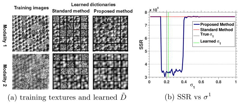
We create multimodal textures by smoothing a given texture with a Gaussian kernel and inverting the intensity of the smoothed image. Fig. 2 shows an example of our generated multimodal textures. We generate both training and testing multimodal textures from Fig. 2, i.e. use half of the multimodal textures for training (add noise as non-correspondence regions) and the other half of the multimodal textures for testing. We extract 10×10 image patches in both training images, and add ‘noise’ with non-corresponding image patches to replace corresponding patches. The σ for the Gaussian noise is set to 0.2.

Fig. 2.

D̃ is learned from training images with Gaussian noise (left). Standard method cannot distinguish corresponding patches and non-corresponding patches while our proposed method can remove non-corresponding patches in the dictionary learning process. The curve (right) shows the robustness with respect to σ₁. The vertical green dashed line indicates the learned σ₁.

We test how σ₁ influences our dictionary learning method at a fixed noise level p(h = 1) = 0.5. Fig. 2 shows the result. In practice, we can either learn σ₁ with an EM algorithm or manually choose it. When σ₁ is close to 0.2 (the σ for the noise), to be specific, σ₁ ∈ (0.15, 0.4), we get consistently lower SSRs. This indicates that our algorithm is robust for a wide range of σ₁ values and noise. For σ₁ < 0.15, all the patches are considered as corresponding patches while for σ₁ > 0.4, all the patches are classified as non-corresponding patches. Our method has the same performance as the standard method in [3] in these two cases. The learned multimodal dictionaries are illustrated in Fig. 2 showing that our algorithm successfully removes non-corresponding patches.

4.2 Synthetic Experiment on Multimodal Microscope Images

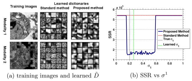
We also test the proposed algorithm on correlative microscope images. We have 8 pairs of Scanning Electron Microscopy (SEM) and confocal images. Image pairs have been aligned with fiducials. Fig. 3 (a) illustrates an example of SEM/confocal images. We add non-corresponding patches using the same method as in sec. 4.1. Fig 3 (a) shows the results. The dictionary learned with our method shows better structure and less noise compared with the standard dictionary learning method. Fig. 3 (b) shows the interaction between σ₁ and SSR with fixed p(h = 1) = 0.5. For σ₁ < 0.16, all the image patches are categorized as corresponding patches while for σ₁ > 0.6, all the patches are classified as non-corresponding patches. Our method has the same performance as the standard method under these conditions. We observe a large range of σ₁ values resulting in improved reconstruction results indicating robustness.

Fig. 3.

D̃ is learned from training SEM/confocal images with Gaussian noise (left). The curve (right) shows the robustness with respect to σ₁. The vertical green dashed line indicates the learned σ₁.

4.3 Multimodal Registration on Correlative Microscopy

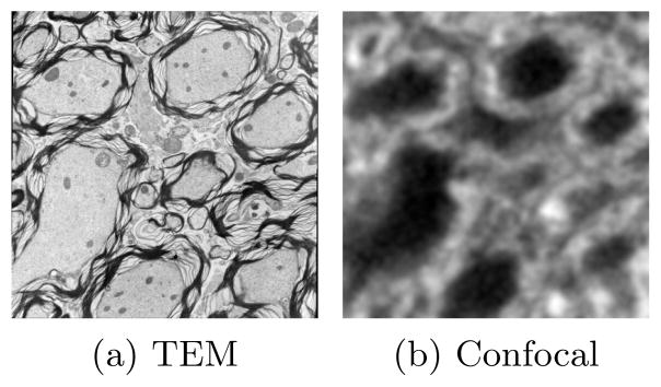
We use the proposed multimodal dictionary learning algorithm for multimodal registration [3]. The multimodal image registration problem simplifies to a monomodal one using the multimodal dictionary in a sparse representation framework. The test data is Transmission Electron Microscopy (TEM) and confocal microscopy. We have six pairs of TEM/confocal images. We train the multimodal dictionary using leave-one-out cross-validation. Fig. 4 shows an example of our test data. We first registered the training images with manually chosen landmarks (no ground truth available), then learned the multimodal dictionary and applied it to predict the corresponding image for a given source image. We resampled the predicted images with up to ± 2.07μm (30 pixels) in translation in the x and y directions (at steps of 10 pixels) and ± 20° in rotation (at steps of 10 degrees). Then we registered the resampled predicted image to the corresponding target using a rigid transformation model. σ₁ is chosen as 0.15 based on cross-validation for the prediction errors in this experiment. Tab. 1 shows a comparison of our method with the method in [3]. The result shows about 15% improvement in prediction error and a statistically significant improvement in registration errors.

Fig. 4.

TEM/Confocal images

Table 1.

Prediction and registration results. Prediction is based on the method in [3], and we use SSR to evaluate the prediction results. Here, MD denotes our proposed multimodal dictionary learning method and ST denotes the dictionary learning method in [3]. The registrations use Sum of Squared Differences (SSD) and mutual information (MI) similarity measures. We report the results of mean and standard deviation of the absolute error of corresponding landmarks in micron (0.069 micron = 1 pixel). The p-value is computed using a paired t-test.

	Metric	Method	mean	std	p-value
Prediction	SSR	MD	6.28 × 104	3.61 × 103
		ST	7.43 × 104	4.72 × 103
Registration	SSD	MD	0.760	0.124	0.0004
		ST	0.801	0.139
	MI	MD	0.754	0.127	0.0005
		ST	0.795	0.140

5 Conclusion

In this paper, we proposed a robust multimodal dictionary learning method based on a probabilistic formulation. We directly model corresponding and non-corresponding multimodal training patches. Our method is based on a variant of the EM algorithm which classifies the non-corresponding image patches and updates the multimodal dictionary iteratively. We validated our method using synthetic and real data. Our algorithm demonstrated its robustness to noise (non-corresponding image patches). We also applied our method to multimodal registration showing an improvement in alignment accuracy compared with the traditional dictionary learning method. The proposed method is expected to be of general use for multimodal dictionary learning. While our method is based on a Gaussian noise model, it can easily be adapted to other noise model such as Poisson noise. Future work will address multimodal dictionary learning in the context of deformable image registration.

References

- 1.Aharon M, Elad M, Bruckstein A. K-svd: An algorithm for designing overcomplete dictionaries for sparse representation. Signal Processing, IEEE Transactions on. 2006;54(11):4311–4322. [Google Scholar]
- 2.Besag J. On the statistical analysis of dirty pictures. Journal of the Royal Statistical Society. Series B (Methodological) 1986:259–302. [Google Scholar]
- 3.Cao T, Zach C, Modla S, Powell D, Czymmek K, Niethammer M. Registration for correlative microscopy using image analogies. Biomedical Image Registration. 2012:296–306. doi: 10.1016/j.media.2013.12.005. [DOI] [PMC free article] [PubMed] [Google Scholar]
- 4.Elad M, Aharon M. Image denoising via sparse and redundant representations over learned dictionaries. Image Processing, IEEE Transactions on. 2006;15(12):3736– 3745. doi: 10.1109/tip.2006.881969. [DOI] [PubMed] [Google Scholar]
- 5.Mairal J, Bach F, Ponce J, Sapiro G. Online dictionary learning for sparse coding. Proceedings of the 26th Annual International Conference on Machine Learning; ACM. 2009. pp. 689–696. [Google Scholar]
- 6.Mairal J, Bach F, Ponce J, Sapiro G, Zisserman A. Supervised dictionary learning. NIPS. 2008:1033–1040. [Google Scholar]
- 7.Monaci G, Jost P, Vandergheynst P, Mailhe B, Lesage S, Gribonval R. Learning multimodal dictionaries. Image Processing, IEEE Transactions on. 2007;16(9):2272–2283. doi: 10.1109/tip.2007.901813. [DOI] [PubMed] [Google Scholar]
- 8.Neal R, Hinton G. A view of the em algorithm that justifies incremental, sparse, and other variants. NATO ASI Series D Behavioural and Social Sciences. 1998;89:355– 370. [Google Scholar]
- 9.Roy S, Carass A, Prince J. Information Processing in Medical Imaging. Springer; 2011. A compressed sensing approach for mr tissue contrast synthesis; pp. 371–383. [DOI] [PMC free article] [PubMed] [Google Scholar]
- 10.Wright J, Yang A, Ganesh A, Sastry S, Ma Y. Robust face recognition via sparse representation. Pattern Analysis and Machine Intelligence, IEEE Transactions on. 2009;31(2):210–227. doi: 10.1109/TPAMI.2008.79. [DOI] [PubMed] [Google Scholar]
- 11.Yang J, Wright J, Huang T, Ma Y. Image super-resolution via sparse representation. Image Processing, IEEE Transactions on. 2010;19(11):2861–2873. doi: 10.1109/TIP.2010.2050625. [DOI] [PubMed] [Google Scholar]