Weighted Functional Boxplot with Application to Statistical Atlas Construction

Abstract

Atlas-building from population data is widely used in medical imaging. However, the emphasis of atlas-building approaches is typically to compute a mean/median shape or image based on population data. In this work, we focus on the statistical characterization of the population data, once spatial alignment has been achieved. We introduce and propose the use of the weighted functional boxplot. This allows the generalization of concepts such as the median, percentiles, or outliers to spaces where the data objects are functions, shapes, or images, and allows spatio-temporal atlas-building based on kernel regression. In our experiments, we demonstrate the utility of the approach to construct statistical atlases for pediatric upper airways and corpora callosa revealing their growth patterns. Furthermore, we show how such atlas information can be used to assess the effect of airway surgery in children.

1 Introduction

Atlas-building from population data has become an important task in medical imaging to provide templates for data analysis. Numerous methods for atlas-building exist, ranging from methods designed for cross-sectional, longitudinal, and random design data. These approaches typically estimate a representative data object (e.g., shape, surface, image) for the population; e.g., a population mean [7] or median [3] with respect to spatial deformations and appearance. This is a restrictive representation, as much of the population data is discarded. In the literature, this has been acknowledged, e.g., by multi-atlas approaches [1] or manifold learning approaches [5] which retain population information by using sets of representative objects or by identifying a low-dimensional data representation.

An alternative strategy to retain population information is to represent additional aspects of the full data distribution, such as percentiles, the robust minimum and maximum, variance, confidence regions and outliers as captured by a boxplot for scalar-valued data. The functional boxplot [12] allows just this for functions. Similarly, we can use it to treat shapes and images (see Fig. 1) and therefore as a simple method to augment atlases with additional population information while avoiding restrictive point-wise analyses of data-objects. Note that we focus in this paper on augmenting atlases with statistical information and assume a given spatial alignment of data objects. However, the method could be extended to build order statistics from low-dimensional manifold embeddings where point-wise analysis becomes meaningful as each point then represent a full data object.

Fig. 1.

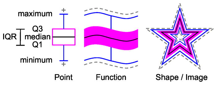
Illustration of boxplots for points, functions, shapes and images. Median (middle black line), confidence region (magenta) and the maximum non-outlying envelope (two outward blue lines). The gray dash lines are the outliers.

As subject data typically has associated individual characteristics (e.g., age, weight, gender) we want to be able to compute the statistical information continuously parameterized by these characteristics. For example, given a subject at a particular age we want to compute subject age-specific confidence regions to assess similarity with respect to the full data population.

We make the following contributions in this paper:

• We develop a weighted variant of the functional boxplot in Sec. 2. This allows us for example to use kernel-regression to build spatio-temporal atlases.

• We show the effectiveness of the method in comparison to point-wise analysis in Sec. 3 highlighting the importance of object-oriented data analysis.

• We show applicability of the method to functions, shapes, and images in Sec. 4 and demonstrate how an atlas can robustly be augmented with statistical data for two applications: capturing changes in pediatric airway development and changes of the corpus callosum over time. We also briefly sketch how our method could be used to build order-statistics on manifolds.

• We show the use of our method for airway surgery assessment in children in Sec. 5, where an age-adapted atlas can be used to quantify how “normal” a child suffering from airway obstruction is before and after surgery.

2 Weighted functional boxplots and atlas-building

The population of data-objects for atlas building could be functions, shapes, and images with associated to subjects characteristics. As an example, we consider subject age and demonstrate spatio-temporal atlas-building as a combination of weighted functional boxplots and kernel smoothing.

2.1 Atlas building with kernel regression

Given spatially aligned data objects we want to capture population changes for example with respect to age. This can be achieved through kernel regression which essentially assigns weights to data-objects with respect to the regressor (say a desired age ā). We can use for example a Gaussian weighting function w_i(a_i; σ, ā) = ce^{(a_i−ā)2/2σ2}, where a_i is the age for the observation i, σ is the standard deviation for the Gaussian distribution and c a normalization constant to assure that the weights sum up to one. For scalar-valued data the weights can simply be used to define a weighted mean. When deformations are of concern they can be used as weights in an atlas-building procedure for images [2]. Here, we are interested in augmenting an atlas with functional statistical information and hence need to develop a weighted functional boxplot to obtain a regressed median (which is an actual data-object from the population), α central region, maximum non-outlying envelop, and outliers.

2.2 Weighted functional boxplots

To define a weighted functional boxplot consistent with the functional boxplot introduced by Sun et. al. [12] requires the definition of a consistent weighted band depth for functional data. This imposes an ordering of the weighted observations (data-objects) with respect to the (to be determined) central data-object.

Weighted band-depth

The functional boxplot is defined through the concept of band-depth [9, 12]. Since each observation has a different weight, we need to define a weighted band-depth. Such a definition immediately defines the weighted functional boxplot. To motivate our choice, assume we want to compute a standard weighted median of scalar values, which is given by ${\mu }^{\ast }=\underset{\mu }{\text{argmin}}{\sum }_{i=1}^n{w}_i\mid x_i-\mu \mid$, where μ is the sought-for median, {x_i} are the measurements, and w_i > 0 are weights for the individual measurements. Assume that all weights are natural numbers, i.e., w_i ∈ ℕ⁺. This can be achieved exactly for arbitrary rational w_i and approximately in general by multiplying the energy with a suitable constant and does not change the minimizer. Hence, we replace the weighted problem with the equivalent unweighted minimization problem ${\mu }^{\ast }=\underset{\mu }{\text{argmin}}{\sum }_{i=1}^n{\sum }_{j=1}^{m_i}\mid x_i-\mu \mid$, where the individual measurements are simply repeated based on their multiplicities, m_i = w_i. Similarly, repeating observations (according to weight), the sampled band-depth can be written as

$$B{D}_{\overline{n}}^{(j)}(y)=\frac{1}{C}{\sum }_{1\le i_1\le i_2<\cdots <i_j\le \overline{n}}I\{G(y)\subseteq B({\overline{y}}_{i_1},\cdots ,{\overline{y}}_{i_j})\},$$ (1)

$$\mathrm{s}.\mathrm{t}.\{{\overline{y}}_{i_1},\cdots ,{\overline{y}}_{i_j}\}\text{contains}\text{unique}\text{observations}.$$ (2)

where C is a normalization constant (i.e., contains the number of admissible permutations), I denotes the indicator function, G(y) is the graph of the function y(x), and B is the band delimited by the observations given as its arguments. We made use of the fact that, according to our definition, we only want to consider unique observations for the depth measure; the {ȳ_i} contain the original observations {y_i}, but according to their respective multiplicity given by the weights. Rewriting the sampled band-depth as

$${\mathit{WBD}}_n^{(j)}(y)=\frac{{\sum }_{1\le i_1<i_2<\cdots <i_j\le n}{w}_{i_1}{w}_{i_2}\cdots w_{i_j}I\{G(y)\subseteq B(y_{i_1},\cdots ,y_{i_j})\}}{{\sum }_{1\le i_1<i_2<\cdots <i_j\le n}{w}_{i_1}{w}_{i_2}\cdots w_{i_j}}$$ (3)

defines the weighted band-depth and generalizes to non-natural-numbered weights w_i ∈ ℝ⁺. In fact, this is a “natural ” way to define a weighted band-depth and, in further consequence, a weighted functional boxplot. Computing the weighted band-depth in this way is intuitive, as only bands with large weights for all its individual observations have a large impact. Furthermore, this weighted version can be also adapted to the modified band-depth proposed in [12], i.e.,

$${\mathit{WMBD}}_n^{(j)}(y)=\frac{{\sum }_{1\le i_1<i_2<\dots <i_j\le n}{w}_{i_1}{w}_{i_2}\cdots w_{i_j}{\lambda }_m\{A(y;y_{i_1},\dots ,y_{i_j})\}}{{\sum }_{1\le i_1<i_2<\dots <i_j\le n}{w}_{i_1}{w}_{i_2}\cdots w_{i_j}}$$ (4)

where A_j (y) ≡ A(y; y_i1, …, y_ij) ≡ {x ∈ ℝ^m : min_{r=i1, …, ij} y_r (x) ≤ y(x) ≤ max_{r=i1, …, ij} y_r (x)}, m is the observation’s dimension, λ_m(y) = λ(A_j(y))/λ(ℝ^m) and λ is the Lebesgue measure on ℝ^m.

With the above definitions, the band depths of all the sampled observations can be calculated and ranked in descending order, y_[1](x) ≥ … ≥ y_[n](x). y_[1](x) is the deepest observation and regarded as the median of the population, whereas y[n](x) is the most outlying observation which is a potential outlier.

α central region

The concept of central region was introduced in [8]. We define the α central region for the weighted functional boxplot based on the weights of observations. The band of the α central region is delimited by the α proportion of all weights, i.e., the accumulated weights of the first p deepest observations

$${\mathit{WCR}}_{\alpha }=\{(\mathbf{x},y,(\mathbf{x})):\underset{r=1,\dots ,p}{\mathit{min}}{y}_{[r]}(\mathbf{x})\le y(\mathbf{x})\le \underset{r=1,\dots ,p}{\mathit{max}}{y}_{[r]}(\mathbf{x}),(\sum _{r=1,\dots ,p-1}{w}_{[r]}<\alpha )\cap (\sum _{r=1,\dots ,p}{w}_{[r]}\ge \alpha ),0\le \alpha \le 1\},$$ (5)

where w_[r] corresponds to the weight for the r-th deepest observation. When α = 0.5, (5) corresponds to the 50% central region WCR_0.5. In practice, the 50% central region is commonly chosen as the confidence region for analysis because it 1) is a robust range for interpretation and 2) enables visualization of the data spread which is less affected by outliers or extreme-values.

Outlier detection

In classical boxplots, the outliers can be detected by the 1.5 IQR (interquartile range). This is comparable to 1.5 times the height of the 50% central region for the weighted functional boxplot. Besides, the weights of the observations also need to be taken into consideration during outlier detection. According to the probability density function for a boxplot based on a normal distribution, the IQR is equal to the 50% distribution and the 1.5 IQR covers the 99.3% distribution. Hence, we define fences by combining the one of the 1.5 IQR with the accumulated weights consistent with the 1.5 IQR of the normal distribution, and any objects outside the fences will be flagged as outliers:

$$\begin{array}{l}{C}_{\mathit{fences}}=\{(\mathbf{x},y(\mathbf{x})):\mathit{max}(mi{n}_{r=1,\dots ,q}{y}_{[r]}(\mathbf{x}),\mathit{min}({\mathit{WCR}}_{\alpha })-1.5\ast \mathit{IQR})\cup \\ \mathit{min}(ma{x}_{r=1,\dots ,q}{y}_{[r]}(\mathbf{x}),\mathit{max}({\mathit{WCR}}_{\alpha })+1.5\ast \mathit{IQR}),\\ (\sum _{r=1,\dots ,q-1}{w}_{[r]}<\beta )\cap (\sum _{r=1,\dots ,q}{w}_{[r]}\ge \beta ),\beta =0.993\}\end{array}$$ (6)

3 Comparisons of boxplots for analysis

We compare atlases built by 1) weighted point-wise boxplots and 2) functional boxplots, using synthetic observations defined by

$$y_i(x)=500\ast (1+\mathit{sin}(2\pi x+0.1\pi i))+2\ast {\mathit{age}}_i,$$

where x ∈ [0, 1], i is the curve index and age_i its age. Fig. 2 shows the curves colored by age.

Fig. 2.

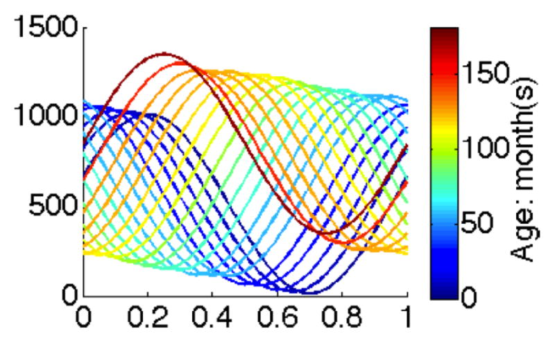
Observations.

Fig. 3(a) shows an atlas built with the weighted point-wise boxplot including four typical percentiles and the point-wise median. While the median curve follows the overall population trend, it is not close to any of the observations because weighted boxplots applied in a point-wise manner to a population of functions disregard the spatial aspect of the functional data. In contrast, our method 1) provides a median curve which corresponds to a curve in the data set, and 2) allows for the computation of functional outliers (gray dashed lines) which results in a more robust statistical description for the atlas.

Fig. 3.

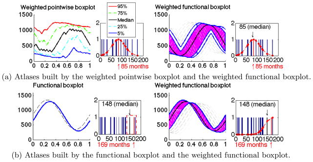
Comparisons of boxplots on the synthetic data.

To construct an atlas at a particular age using standard functional boxplots, we use a uniform window to pick curves centered around the age of interest. As shown in Fig. 3(b), only two curves are available in the uniform window for atlas-building with functional boxplots, and one of them is flagged as an outlier. This atlas includes little information about the population. The atlas built using the weighted functional boxplot (with a Gaussian window size that is comparable to the uniform one according to [10]) captures the population data much better as it does not suffer from the local data sparsity and makes use of all the data.

4 Applications

4.1 Data

The data objects for the weighted functional boxplot can for example be functions, shapes and images (with shapes and images converted to long vectors).

Functions

Our first application is the construction of a pediatric airway atlas for normal subjects to assess airway malformations (subglottic stenosis (SGS)). The observations are a population of 1D functions describing airway cross-sectional areas parameterized along the centerline of the airway. Functions are generated from 3D CT data for 44 normal subjects using the approach in [6] followed by landmark based spatial alignment [11]. We focus the analysis on the region between the true vocal cord and the trachea carina, where SGS locates.

Shapes

The second application is to build a corpus callosum atlas and to explore shape changes with age. The observations are a collection of 32 corpus callosum shapes of varying ages from [4]. Each shape is represented by 64 2D boundary points. We perform affine alignment before atlas constructions.

Images

The third application is to understand age-related changes of the corpus callosum using binary images of the corpus callosum segmentations. The images are converted from the aligned corpus callosum shapes.

4.2 Comparison with point-wise boxplots

We compare the functional boxplot to the point-wise approach on above real datasets to further demonstrate the advantages of our method. Fig. 4 shows the median (the black curve) and the confidence region (the 50% central region, magenta) for both point-wise and functional boxplots. We count the number of data objects inside the confidence region: for the point-wise boxplots only 5 (of 44) functions and none of the shapes or images are fully within the confidence region. However, the functional boxplots by construction achieves a confidence region containing 50% of the data objects. Hence it is a more intuitive representation of true data-object variation. To construct the point-wise confidence regions for shapes we locally compute distances with respect to the median point which establishes an (unsigned) ordering. The confidence region is then the convex hull of the closest half of the points. This strategy would extend to constructing approximate confidence regions with respect to manifold embedding coordinates.

Fig. 4.

Comparison between point-wise (top) and functional (bottom) boxplots on functions, shapes and images (from left to right).

4.3 Atlas Construction with weighted functional boxplots

The weighted functional boxplot is used to build a pediatric airway atlas with variance σ = 30 months for the weighting function, Fig. 5(a), and the corpus callosum shape/image atlases with σ = 10 years, Fig. 5(b). The pediatric airway atlases capture increases in cross-sectional airway area with age which is consistent with the growth pattern for pediatric airways and indicates the necessity of building an age-adapted atlas as a reference. The corpus callosum atlases reveal the thinning trend in the shape and the decreasing volume in the image with age, especially at the anterior and posterior parts consistent with [4].

Fig. 5.

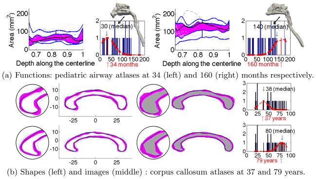
Age-adapted atlases for functions, shapes, and images.

5 Assessment with Statistical Atlas

To test the utility of the statistical atlas built by weighted functional boxplots we show (Fig. 6) airway changes of a SGS subject before (at 9 months) and after (at 20 months) surgery compared to the age-matched normal control airway atlas. Before treatment, there is a constricted region outside the atlas; after treatment, the airway size increases and the corresponding curve is almost entirely within the maximal non-outlying envelope, indicating a successful surgery.

Fig. 6.

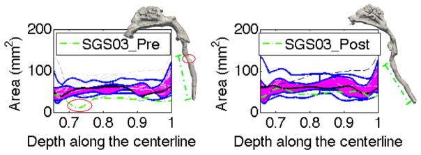
Airway changes for a subject pre- and post-surgery (green lines) compared to the age-matched atlas. The stenosis of the airway is marked by the red ellipse on the pre-surgery geometry and no stenosis exists in the post-surgery geometry.

6 Discussion and Conclusions

We proposed a method to compute weighted functional boxplots and use it for spatio-temporal atlas building. We applied it to construct a pediatric airway atlas to assess children with subglottic stenosis and a corpus callo-sum atlas capturing aging. The proposed method is general, easy to compute, and allows robust statistical description of functional, shape, and image data.

References

- 1.Aljabar P, Heckemann R, Hammers A, Hajnal J, Rueckert D. Multi-atlas based segmentation of brain images: Atlas selection and its effect on accuracy. NeuroImage. 2009;46:726–739. doi: 10.1016/j.neuroimage.2009.02.018. [DOI] [PubMed] [Google Scholar]
- 2.Davis BC, Fletcher PT, Bullitt E, Joshi S. Population shape regression from random design data. International journal of computer vision. 2010;90(2):255–266. [Google Scholar]
- 3.Fletcher P, Venkatasubramanian S, Joshi S. The geometric median on Riemannian manifolds with application to robust atlas estimation. NeuroImage. 2009;45(Suppl 1):S143–S152. doi: 10.1016/j.neuroimage.2008.10.052. [DOI] [PMC free article] [PubMed] [Google Scholar]
- 4.Fletcher T. Geodesic regression on Riemannian manifolds. 3rd MICCAI workshop on mathematical foundations of computational anatomy; 2011. pp. 75–86. [Google Scholar]
- 5.Gerber S, Tasdizen T, Fletcher PT, Joshi S, Whitaker R. Manifold modeling for brain population analysis. Medical image analysis. 2010;14(5):643–653. doi: 10.1016/j.media.2010.05.008. [DOI] [PMC free article] [PubMed] [Google Scholar]
- 6.Hong Y, Niethammer M, Andruejol J, Kimbel J, Pitkin E, Superfine R, Davis S, Zdanski C, Davis B. A pediatric airway atlas and its application in subglottic stenosis. International symposium on biomedical imaging: from nano to macro; 2013. pp. 1194–1197. [DOI] [PMC free article] [PubMed] [Google Scholar]
- 7.Joshi S, Davis B, Jomier M. Unbiased diffeomorphic atlas construction for computational anatomy. Neuroimage. 2004;23(Suppl 1):S151–S160. doi: 10.1016/j.neuroimage.2004.07.068. [DOI] [PubMed] [Google Scholar]
- 8.Liu R, Parelius J, Singh K. Multivariate analysis by data depth: descriptive statistics, graphics and inference. The annals of statistics. 1999;27:783–858. [Google Scholar]
- 9.López-Pintado S, Romo J. On the concept of depth for functional data. Journal of the American Statistical Association. 2009;104:718–734. [Google Scholar]
- 10.Marron J, Nolan D. Canonical kernels for density estimation. Statistics and probability letters. 1988;7:195–199. [Google Scholar]
- 11.Ramsay J, Silverman B. Functional Data Analysis. Springer; 2005. [Google Scholar]
- 12.Sun Y, Genton M. Functional boxplots. Journal of Computational and Graphical Statistics. 2011;20:316–334. [Google Scholar]