Geodesic Regression for Image Time-Series

Abstract

Registration of image-time series has so far been accomplished (i) by concatenating registrations between image pairs, (ii) by solving a joint estimation problem resulting in piecewise geodesic paths between image pairs, (iii) by kernel based local averaging or (iv) by augmenting the joint estimation with additional temporal irregularity penalties. Here, we propose a generative model extending least squares linear regression to the space of images by using a second-order dynamic formulation for image registration. Unlike previous approaches, the formulation allows for a compact representation of an approximation to the full spatio-temporal trajectory through its initial values. The method also opens up possibilities to design image-based approximation algorithms. The resulting optimization problem is solved using an adjoint method.

1 Introduction

The analysis of image-time series is important to study brain development, aging processes, or tumor growth to name but a few application areas. Being able to establish image correspondences and localize change is essential if global measures are insu cient for analysis. While image registration between image pairs has been extensively researched for decades, considering populations of images is more recent. Here, joint-alignment procedures [6] have become standard tools for cross-sectional population-based image analysis. Lately, methods for longitudinal data analysis have been proposed based on the extension of large-deformation-di eomorphic-metric-mapping (LDDMM) registration to image time-series [4,8] or series of point clouds [9]. Here, only [9] provides a true generative model, since the approach is based on an initial value formulation for the registration of shapes. Initial value formulations have been theoretically discussed for images [7], but only recently solved as initial value problems [11,1].

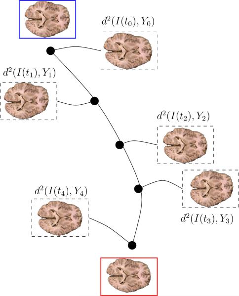
Statistics in the LDDMM setting are most naturally performed on momenta with respect to a mean image [10]. If a piecewise geodesic estimation for a time-series is used, this requires transporting the set of momenta (for each measurement point of a time-series) to a reference coordinate frame (as proposed in [9] for points sets)¹. Instead of reformulating [9] for images using the initial-value formulation for image registration, we investigate the behavior of an approximative time-series model, which generalizes least-square linear regression to the image-valued case. The method (i) is generative, describing a full time-trajectory by an initial image and momentum, (ii) will allow for compact statistical analyses of time series based on sets of initial momenta (one for each time series), (iii) opens up the possibility to design approximative algorithms for image time-series (e.g., an approximative spline, useful for random-design data), and (iv) handles non-uniform sampling in time. We use a second order image-based formulation and minimize the sum of squared distances of a set of measured images to a geodesic (Fig. 1). Once a distance measure is defined, we only need to estimate the change of the sum of squared distances with respect to the initial conditions of the dynamical system. This is accomplished by an adjoint solution method (Sec. 4) motivated by a scalar-valued formulation (Sec. 2) and generalized to the image-valued case (Sec. 3). Sec. 5 presents results, Sec. 6 conclusions.

Fig. 1.

Principle of geodesic regression on the space of images. The interpolation path is determined by the blue and the red images. This geodesic path is maximally close to the dashed images.

2 Dynamic Formulation of Least-Squares Line Fitting

Consider least-squares linear regression from an optimal control viewpoint: Let {y_i} be a set of M measurements at time points {t_i} not necessarily distinct and ${\stackrel{.}{x}}_1=x_2$; ${\stackrel{.}{x}}_2=0$ be the dynamical system where the states denote y-intercept and slope respectively. The goal is to find initial conditions x₁(t₀), x₂(t₀) s.t.

$$E={\int }_{t_0}^{t_{M-1}}{\lambda }_1({\stackrel{.}{x}}_1-x_2)+{\lambda }_2\left({\stackrel{.}{x}}_2\right)+\sum _{i=0}^{M-1}{(x_1\left(t_i\right)-y_i)}^2$$ (1)

is minimized, where the Lagrangian multipliers λ₁ and λ₂ may be discontinuous. The variation yields the state equation and a boundary value problem for λ₁, λ₂

$$\{\begin{array}{cc}-{\stackrel{.}{\lambda }}_1=0,\hfill & {\lambda }_1\left(t_0^{-}\right)=0,{\lambda }_1\left(t_{M-1}\right)=-2(x_1\left(t_{M-1}\right)-y_{M-1}),\hfill \\ -{\stackrel{.}{\lambda }}_2={\lambda }_1,\hfill & {\lambda }_2\left(t_0\right)={\lambda }_2\left(t_{M-1}\right)=0,\hfill \end{array}\phantom{\}}$$

with jump conditions ${\lambda }_1\left(t_i^{-}\right)={\lambda }_1\left(t_i^{+}\right)-2(x_1\left(t_i\right)-y_i)$. The gradients of the energy with respect to the initial conditions are $-{\lambda }_1\left(t_0^{-}\right)={\nabla }_{x_1\left(t_0\right)}E$, −λ₂ = ∇ x₂(t₀)E. We can explicitly solve the equations and obtain the conditions

$$\sum _{i=0}^{M-1}(x_1\left(t_i\right)-y_i)=0,\sum _{i=0}^{M-1}(t_i-t_0)(x_1\left(t_i\right)-y_i)=0.$$

The first condition is a force balance (of model residuals) and the second a moment balance. The dynamic formulation extends to the space of images (Sec. 3). We obtain the mechanical interpretation that λ₁ is the (backward in time) running sum of forces and λ₂ is the (backward in time) running sum of moments. Both need to vanish at optimality. The second-order constraint $({\stackrel{.}{x}}_2=0)$ is necessary to obtain a straight line. Relaxing this constraint, the method falls back to a piecewise geodesic model as currently used in the LDDMM framework.

3 Geodesic Regression on the Space of Images

The LDDMM framework provides a convenient Riemannian setting where geodesics corresponds to straight lines in the scalar case. Geodesics on the space of the deformed images are obtained by minimizing the functional

$$\mathcal{E}\left(v\right)={\int }_0^1{\Vert v\Vert }_V^{2}dt+d^2(I\left(1\right),Y),$$ (2)

where v is a time-dependent velocity field in V , a Reproducing Kernel Hilbert Space (RKHS) of smooth velocity fields; d² denotes a general squared-distance(-like) term. Extending (2) to multiple timepoints leads to piecewise geodesic interpolation. For a single timepoint however, it gives the geodesicity that needs to be enforced for our least squares generalization. The Euler-Lagrange equation for $\mathcal{E}$ is a special case of the EPDiff equation and parametrizes a geodesic in image space given an initial image I(t₀) and an initial momentum p(t₀) [11]:

$$I_t+\nabla I^{T}v=0,p_t+div\left(pv\right)=0,v+K\star (\nabla Ip)=0.\left(\mathrm{EPDiff}\right)$$ (3)

where K is the (translation invariant) smoothing kernel of the RKHS and * the convolution operator. Weighted (w_i ≥ 0) geodesic regression is to minimize

$$E=\langle p\left(t_0\right)\nabla I\left(t_0\right),K\star (p\left(t_0\right)\nabla I\left(t_0\right)\rangle +\sum _{i=0}^{M-1}{w}_i{d}^2(I\left(t_i\right),Y_i)$$ (4)

wrt. the initial conditions (I(t₀), p(t₀)) subject to the EPDi equation (3) that replaces the dynamic line model ${\stackrel{.}{x}}_1=x_2$, ${\stackrel{.}{x}}_2=0$ in Sec. 2. More importantly, the first term (not present in the scalar case) ensures the well-posedness of the model by preventing high frequencies in the time-dependent velocity field.

3.1 Optimality Conditions

Evolution equations for the adjoints are valid piece-wise with jump conditions at measurement instants. Jumps depend on how much a measured image “pulls” at the geodesic. Weights w_i for the measurements allow for the equivalent of locally linear regression [5] on the space of images². We obtain the state equations and the optimality conditions for the adjoints λ^I, λ^p

$$\{\begin{array}{cc}-{\lambda }_t^I-div\left(v{\lambda }^I\right)-div(pK\ast {\lambda }^v)\hfill & =0,\hfill \\ {\lambda }^I\left(t_{M-1}\right)\hfill & =-w_{M-1}{\nabla }_{I\left(t_{M-1}\right)}{d}^2\left(I(t_{M-1},Y_{M-1})\right),\hfill \\ -{\lambda }_t^p-v^T\nabla {\lambda }^p+\nabla I^{T}K\ast {\lambda }^v\hfill & =0,{\lambda }^p\left(t_{M-1}\right)=0,\hfill \\ {\lambda }^I\nabla I-p\nabla {\lambda }^p+{\lambda }^v\hfill & =0,t\in [t_i^{+},t_{i+1}^{-}],i=0\left(1\right)M-2.\hfill \end{array}\phantom{\}}$$

subject to the compatibility conditions

$$\{\begin{array}{cc}{\lambda }^I\left(t_i^{-}\right)={\lambda }^I\left(t_i^{+}\right)-w_i{\nabla }_{I\left(t_i\right)}{d}^2(I\left(t_i\right),Y_i),\hfill & i>0,\hfill \\ {\lambda }^p\left(t_i^{-}\right)={\lambda }^p\left(t_i^{+}\right),\hfill & i>0,\hfill \\ 0={\lambda }^I\left(t_0^{+}\right)-w_i{\nabla }_{I\left(t_0\right)}{d}^2(I\left(t_0\right),Y_0)-2div(p\left(t_0\right)K\ast (p\left(t_0\right)\nabla I\left(t_{0}0\right)),\hfill & i=0,\hfill \\ 0=-{\lambda }^p\left(t_0^{+}\right)+2\nabla I{\left(t_0\right)}^{T}K\ast (p\left(t_0\right)\nabla I\left(t_0\right)),\hfill & i=0.\hfill \end{array}\phantom{\}}$$

For notational convenience define ${\lambda }^I\left(t_0\right)≔{\lambda }^I\left(t_0^{+}\right)-w_0{\nabla }_{I\left(t_0\right)}{d}^2(I\left(t_0\right),Y_0)$, ${\lambda }^p\left(t_0\right)≔{\lambda }^p\left(t_0^{+}\right)$. We obtain the gradients

$$\begin{array}{cc}\hfill & {\nabla }_{I\left(t_0\right)}E=-{\lambda }^I\left(t_0\right)-2div(p\left(t_0\right)K\ast (p\left(t_0\right)\nabla I\left(t_0\right))),\hfill \\ \hfill & {\nabla }_{p\left(t_0\right)}E=-{\lambda }^p\left(t_0\right)+2\nabla I{\left(t_0\right)}^{T}K\ast (p\left(t_0\right)\nabla I\left(t_0\right)).\hfill \end{array}$$

Note that both initial momentum and the initial image are unknowns. To fully define the problem we need to specify the distance measure d² and its gradient.

3.2 Choices for d²

Selecting d² is a design choice. The gradients (wrt. I(t_i)) can be viewed as forces pulling on the geodesic. We discuss the gradients for distances based on the L² metric and LDDMM registration; a metamorphosis approach could also be used.

L², Interpolation-based image-match term

The squared L² distance between images and its (infinite-dimensional) derivative is

$$d^2(J,Y)≔{\Vert J-Y\Vert }^2;{\nabla }_J{d}^2(J,Y)=2(J-Y).$$

Note that other similarity measure such as cross-correlation or mutual-information could also be used. This definition simplifies computations. It is only meaningful if the geodesic is close to the measured images. If large distances are admissible the squared distances can be defined by registration themselves.

Approximation-based inexact image-match term

We use the same second order model as for the regression line for image-to-image registration to define:

$$d^2(J,Y)=\underset{p\left(0\right)}{\mathrm{argmin}}{\langle p\left(0\right)\nabla I\left(0\right)K\star p\left(0\right)\nabla I\left(0\right)\rangle }_{L^2}+\frac{1}{{\sigma }^2}{\Vert I\left(1\right)-Y\Vert }^2,$$ (5)

subject to the EPDi equation with initial image given by I(0) = J. This is a special case of the geodesic regression problem with two images with an L² distance measure. For an optimal set {I* , p* , v, λ^I* , λ^p* , λ^v*}) the gradient of the squared distance measure with respect to J is hence given by

$${\nabla }_J{d}^2(J,Y)=-{\lambda }^I\left(0\right)-2div(p\left(0\right)K\ast (p\left(0\right)\nabla I\left(0\right))).$$

Note the slight abuse of notation, since here λ^I is not the Lagrangian multiplier for geodesic regression, but for the geodesic of the registration problem.

3.3 Mechanical Interpretation

A similar mechanical interpretation as for the scalar-valued case holds. Since the state and the adjoint equations are more involved, we can no longer explicitly solve the optimality conditions. However, the Lagrangian multipliers λ^I can be considered as the generalized running sum of forces and λ^p as the generalized running sum for the moment. The gradients of the squared distance measures with respect to the respective source images can be considered generalized forces. The additional terms appearing in the energy gradients with respect to the initial conditions result from penalizing the length of the geodesic.

4 Numerical Solution

To obtain a solution fulfilling the optimality conditions, we compute the gradients with respect to I(t₀) and p(t₀) through the adjoints. We use a multi-scale approach to speed up convergence. The algorithm proceeds as follows

• 0Specify an initial (I(t₀), p(t₀)).

1. Solve the state equation forward, while saving computed values I(t) and p(t).

2. Solve the adjoint equations backward while applying jump conditions at every time-point with an available measured image.

3. Compute ∇ _I(t0)E and ∇ p(t₀)E from λ^I(t₀), λ^p(t₀), I(t₀) and p(t₀).

4. Use the gradients to update I(t₀) and p(t₀) through a line search.

5. Repeat from step 1 until converged.

We solve the advection equation for I and the scalar conservation law for p using a map-based approach as proposed in [2] to minimize numerical dissipation. We use a similar approach to solve for the adjoints λ^I and λ^p, but treat all terms which cannot be explained by advection or scalar conservation as source terms which are added to the solutions at each time step as in [11,8]. If it is desired to obtain a least squares fit such that I(t₀) = I₀ (where I₀ is a given fixed initial image) the gradient with respect to I(t₀) can simply be disregarded. In the scalar case this amounts to fixing the y intercept at t₀ and searching for the best slope.

5 Experimental Results

We tested the geodesic regression model using synthetic and real images. Note that this paper focuses on the formulation and solution of the geodesic regression model. Validation in the context of population studies will be future work.

5.1 Synthetic Images

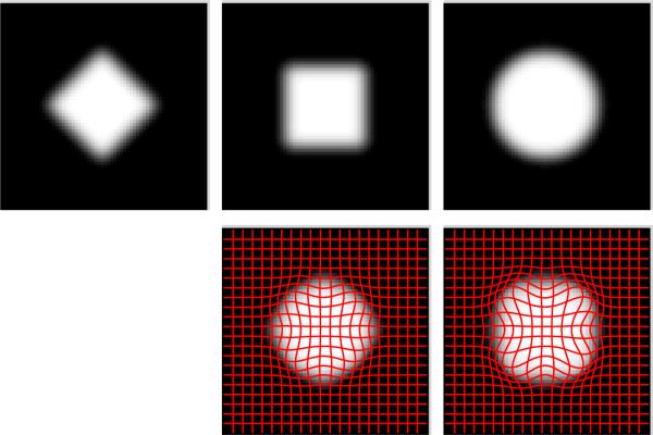
We applied the method to a translating circle with w_i = 0.1 and a Gaussian kernel K with σ = 4 pixels. Fig. 2 shows the original images and the geodesic regression results when updating initial momentum and the initial image. Since the displacements between consecutive images is small we used the L² distance. The geodesic regression captures the translation well. As expected for a fluid registration non-uniform compressions and dilations occur. Fig. 3 shows an example geodesic regression trajectory for a fixed initial template through three distinct geometric objects. Since this is an approximative algorithm, the shapes are not perfectly recovered, but instead an intermediate solution is obtained, which approximates the square as a shape in-between the circle and the diamond-shape. The size of all synthetic images is 64×64 pixels.

Fig. 2.

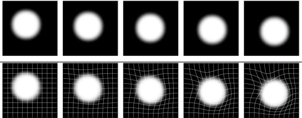
Translation experiment and results for geodesic regression with initial image and momentum free. The translation is well captured.

Fig. 3.

Geodesic regression result with initial image fixed. The resulting trajectory is a compromise between the shapes. A perfect match of the square and the circle would require a local contraction (with respect to the diamond shape) followed by an expansion, which cannot be expressed by the approximative model.

5.2 Real Images: Brain Slices from the OASIS Database

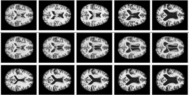
To illustrate the behavior for real images, we took 5 brain slices (176×208 pixels) from 5 subjects at different ages from the OASIS database and applied geodesic regression with w_i = 10 and a Gaussian kernel with σ = 5 pixels using the L² distance. Cases were selected to exhibit an expansion of the ventricles. Since the ventricle topology is different for the subjects, perfect matching cannot be achieved. Even though large scale deformations were present, geodesic regression approximates the temporal evolution of the ventricles. This experiment illustrates that reasonable approximations can be obtained. Computing the geodesic from young to old is numerically challenging, because of the large expansions occurring, which need to be represented by relatively few grid cells in the image. Fig. 5 therefore also shows the estimation results when the geodesic is represented in the space of the oldest subject. Computed deformations are better behaved, because they are easier to represent numerically. In comparison to time-series approaches estimating piece-wise geodesics [8,4], geodesic regression results in a smooth temporal evolution. This is shown in Fig. 4 which compares a coronal cross section (through the ventricles) for the slices over time. Kinks are visible for the piece-wise geodesic, but not for the geodesic regression approach.

Fig. 5.

Brain slices of subjects with increasing age (left to right, 38, 52, 58, 73, 81 [years]) and geodesic regression results. Results with initial conditions in the space of the 38 year old (middle row) and the 81 year old (bottom row) subject.

Fig. 4.

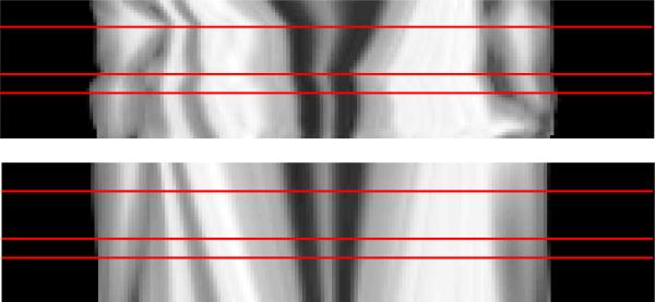
Coronal cross sections through ventricles for piecewise-geodesic approach (top) and for geodesic regression (bottom) with fixed initial image.

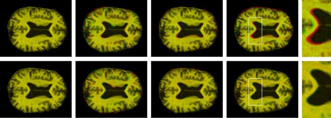
Much smaller changes are expected for longitudinal data. Fig. 6 shows four slices (128×161 pixels) for a longitudinal dataset from the OASIS database. Changes are subtle and most easily seen around the ventricles. The top row shows overlays with respect to the youngest image and illustrates the increase in ventricle size. The ventricle expansion is well captured by geodesic regression.

Fig. 6.

Brain slices for longitudinal subject data (left to right, age: 67, 68, 71, 73 [years]). Top: original images overlaid with image at age 67. Bottom: geodesic regression results overlaid with original images. Yellow indicates agreement. Zoom in to view.

6 Discussion and Conclusions

We proposed a generative model for image time-series, where trajectories are fully parametrized by their initial conditions. To measure distances from the regression geodesic we proposed an L² and a registration-based distance and integrated them into an adjoint solution method. Geodesic regression is an approximative estimation method, which opens possibilities for other approximation methods on the space of images (e.g., approximating splines). We addressed how to estimate an individual trajectory. To perform statistical analysis for populations requires comparing the initial momenta in a common coordinate system, which can be achieved by transporting the initial momenta to a common atlas-space [12]. Geodesic regression simplifies statistical analysis, because of its compact representation of image time-series. It generalizes to piecewise geodesic approximations by concatenating geodesic regressions at specified time-points. This allows standardized representations to compare time-series data with non uniform temporal sampling.

References

- 1.Ashburner J, Friston K. Diffeomorphic registration using geodesic shooting and Gauss-Newton optimisation. Neuroimage. 2011;55(3):954–967. doi: 10.1016/j.neuroimage.2010.12.049. [DOI] [PMC free article] [PubMed] [Google Scholar]
- 2.Beg M, Miller M, Trouvé A, Younes L. Computing large deformation metric mappings via geodesic flows of diffeomorphisms. IJCV. 2005;61(2):139–157. [Google Scholar]
- 3.Davis B, Fletcher P, Bullitt E, Joshi S. Population shape regression from random design data. ICCV. 2007:1–7. [Google Scholar]
- 4.Durrleman S, Pennec X, Trouvé A, Gerig G, Ayache N. Spatiotemporal atlas estimation for developmental delay detection in longitudinal datasets. In: Yang GZ, Hawkes D, Rueckert D, Noble A, Taylor C, editors. MICCAI. LNCS. Vol. 5761. Springer; 2009. pp. 297–304. [DOI] [PMC free article] [PubMed] [Google Scholar]
- 5.Fan J. Local linear regression smoothers and their minimax efficiencies. The Annals of Statistics. 1993;21(1):196–216. [Google Scholar]
- 6.Joshi S, Davis B, Jomier M, Gerig G. Unbiased diffeomorphic atlas construction for computational anatomy. Neuroimage. 2004;23:S151–S160. doi: 10.1016/j.neuroimage.2004.07.068. [DOI] [PubMed] [Google Scholar]
- 7.Miller MI, Trouve A, Younes L. Geodesic shooting for computational anatomy. Journal of Mathematical Imaging and Vision. 2006;24:209–228. doi: 10.1007/s10851-005-3624-0. [DOI] [PMC free article] [PubMed] [Google Scholar]
- 8.Niethammer M, Hart G, Zach C. Conference on Decision and Control (CDC) IEEE; 2009. An optimal control approach for the registration of image time series. pp. 2427–2434. [Google Scholar]
- 9.Qiu A, Albert M, Younes L, Miller M. Time sequence diffeomorphic metric mapping and parallel transport track time-dependent shape changes. NeuroImage. 2009;45(1):S51–S60. doi: 10.1016/j.neuroimage.2008.10.039. [DOI] [PMC free article] [PubMed] [Google Scholar]
- 10.Vaillant M, Miller MI, Younes L, Trouvé A. Statistics on diffeomorphisms via tangent space representations. Neuroimage. 2004;23:S161–S169. doi: 10.1016/j.neuroimage.2004.07.023. [DOI] [PubMed] [Google Scholar]
- 11.Vialard FX, Risser L, Rueckert D, Cotter CJ. Diffeomorphic 3D image registration via geodesic shooting using an efficient adjoint calculation. 2011. preprint.
- 12.Younes L, Qiu A, Winslow RL, Miller MI. Transport of relational structures in groups of diffeomorphisms. Journal of Mathematical Imaging and Vision. 2008;32:41–56. doi: 10.1007/s10851-008-0074-5. [DOI] [PMC free article] [PubMed] [Google Scholar]