Practical Guidance for Conducting Mediation Analysis With Multiple Mediators Using Inverse Odds Ratio Weighting

Abstract

Despite the recent flourishing of mediation analysis techniques, many modern approaches are difficult to implement or applicable to only a restricted range of regression models. This report provides practical guidance for implementing a new technique utilizing inverse odds ratio weighting (IORW) to estimate natural direct and indirect effects for mediation analyses. IORW takes advantage of the odds ratio's invariance property and condenses information on the odds ratio for the relationship between the exposure (treatment) and multiple mediators, conditional on covariates, by regressing exposure on mediators and covariates. The inverse of the covariate-adjusted exposure-mediator odds ratio association is used to weight the primary analytical regression of the outcome on treatment. The treatment coefficient in such a weighted regression estimates the natural direct effect of treatment on the outcome, and indirect effects are identified by subtracting direct effects from total effects. Weighting renders treatment and mediators independent, thereby deactivating indirect pathways of the mediators. This new mediation technique accommodates multiple discrete or continuous mediators. IORW is easily implemented and is appropriate for any standard regression model, including quantile regression and survival analysis. An empirical example is given using data from the Moving to Opportunity (1994–2002) experiment, testing whether neighborhood context mediated the effects of a housing voucher program on obesity. Relevant Stata code (StataCorp LP, College Station, Texas) is provided.

Mediation analyses are crucial for understanding causal relationships and identifying possible intervention points. The field of mediation research has recently exploded, both conceptually and methodologically (1–19). In this article, we outline a new approach utilizing inverse odds ratio weighting (IORW) to evaluate natural direct and indirect effects (8). The benefits of IORW are multifold. It easily accommodates multiple mediators regardless of their scale and improves on recent parametric mediation techniques that fit a regression model for the outcome, given the exposure, mediators, and covariates, and a model for the multivariate density of mediators given exposure and covariates. Unlike the parametric approach, which has been implemented in restricted settings, IORW is universal (i.e., easily implemented with any standard regression model). In this article, we present the IORW method for epidemiologic audiences and offer Stata code (StataCorp LP, College Station, Texas) with which to implement it.

COUNTERFACTUAL-BASED APPROACHES AND LIMITATIONS OF EXISTING TECHNIQUES

The counterfactual-based approach to mediation defines direct and indirect effects in a nonparametric framework, readily accommodating nonlinearities and interactions involving exposure, mediators, and confounders. Pearl (2, 7) articulated formal assumptions under which natural direct and indirect effects are identified, demonstrating that such effects can be computed from observational data under certain assumptions entailing no residual confounding (7) using the mediation formula (see Web Appendix 1, available at http://aje.oxfordjournals.org/). Since Pearl's seminal contribution, the causal mediation literature has focused on developing estimation strategies for computing the mediation formula. Approaches include fully parametric methods (1, 7, 9, 10), semiparametric methods (6, 11–16), and some doubly and multiply robust methods that are less sensitive to model misspecification (6, 14, 17).

The parametric mediation approach posits models for the outcome regression on exposure, mediator, and preexposure confounders. This reduces to Baron and Kenny's classical approach in linear models with no exposure-mediator interaction (4, 20). Recently proposed parametric approaches also apply in the presence of exposure-mediator interactions or with a nonlinear link function, when the Baron and Kenny decompositions are incorrect (9). Parametric approaches can have restrictions on their application. For instance, VanderWeele and Vansteelandt (21) recently developed a parametric (regression-based) mediation method for multiple mediators which can be used for rare, binary outcomes but with the restriction that all mediators are continuous. A method created by Lange et al. (22) relies on a model for the joint density of the mediators, which may be a daunting task for multiple mediators of mixed variable type (e.g., binary, continuous, counts). (Also see Hong and Nomi (23) for a closely related approach.) If the goal is to decompose an exposure effect conditional on covariates, Tchetgen Tchetgen (8) cautions against using the parametric mediation formula if 1) either the outcome or the mediator models use a nonlinear link or 2) there are multiple mediators. Both situations are common.

In situation 1, direct, indirect, and total effects obtained with the parametric mediation formula will often be difficult to interpret given the unorthodox scale induced by the link function (8). Situation 2 requires building a model for the mediator density, possibly involving discrete and continuous components, which is a nontrivial modeling task that becomes increasingly difficult as the number of mediators increases. For instance, even if one had 10 continuous mediators and one assumed that they were normally distributed, one would need to fit a regression for each mediator on exposure and covariates. One would also need data on the variance of each residual and correlations between the residuals (requiring 45 correlation coefficients ((10 × 9)/2)). This method could be computationally prohibitive. An additional difficulty arises when specifying the outcome if interactions exist among any subset of mediators, covariates, and the exposure. Whether to specify such interactions can rarely be decided on the basis of prior knowledge, and empirical tests of interactions involving multiple factors are notoriously underpowered (24, 25).

Here, we abandon the parametric mediation strategy and present Tchetgen Tchetgen's (8) IORW approach. IORW is a simple alternative, is applicable even in the context of nonlinear links, and circumvents the difficulties of modeling the joint density of multiple mediators.

Identification

Suppose independent and identically distributed data are observed for n subjects with outcome Y, binary exposure E, and mediator M, which temporally succeeds the exposure and precedes the outcome, and C is the vector of preexposure variables that confound the relationship between (E, M) and Y (as in the causal directed acyclic graph shown in Figure 1). To define natural direct and indirect effects in causal terms requires defining counterfactuals. Assume that for every level of the exposure and mediator, there exists a counterfactual or potential outcome Y_e,m corresponding to the value of the outcome had exposure and mediator taken values e and m, respectively. Likewise, the counterfactual variable M_e corresponds to the value the mediator would have had if exposure had been e.

Figure 1.

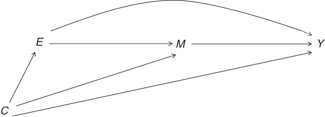
Mediation model showing measured confounding of the exposure, mediator, and outcome. E denotes the binary exposure; M denotes the mediator, which temporally succeeds the exposure and precedes the outcome; and C is the vector of preexposure variables that confound the relationship between (E, M) and Y. Identifying assumptions include the assumption that there is no unmeasured confounding of the effects of the 1) exposure on the mediator, 2) mediator on the outcome, or 3) exposure on the outcome upon conditioning on preexposure confounders. We also assume that there are no confounding variables affected by the exposure. This directed acyclic graph demonstrates a generic causal structure, although in our empirical example with Moving to Opportunity data, there is no arrow from C to E, as E is randomly assigned.

Decomposition of the total effect of the exposure on the outcome on the mean scale into natural direct and indirect effects is

$$\begin{array}{rl}{\gamma }_{\mathrm{total}}(C)& =g^{-1}\{\mathbb{E}(Y_{e=1}|C)\}-g^{-1}\{\mathbb{E}(Y_{e=0}|C)\}\\ & =g^{-1}\{\mathbb{E}(Y_{e=1,M_{e=1}}|C)\}-g^{-1}\{\mathbb{E}(Y_{e=0,M_{e=0}}|C)\}\\ & =g^{-1}\{\mathbb{E}(Y_{e=1,M_{e=1}}|C)\}-g^{-1}\{\mathbb{E}(Y_{e=1,M_{e=0}}|C)\}\\ & +g^{-1}\{\mathbb{E}(Y_{e=1,M_{e=0}}|C)\}-g^{-1}\{\mathbb{E}(Y_{e=0,M_{e=0}}|C)\}\\ & ={\gamma }_{\mathrm{indirect}}(C)+{\gamma }_{\mathrm{direct}}(C),& \end{array}$$ (1)

where 𝔼 stands for expectation and g⁻¹ is a user-specified, possibly nonlinear link function. This decomposition reveals that identification of natural direct and indirect effects requires identification of the conditional mean of the counterfactuals Y_e, M_e* within levels of C, where (e, e*) ∈ {0,1}².

Assumptions

Under Pearl's nonparametric structural equation model interpretation of the causal directed acyclic graph in Figure 1, natural direct and indirect effects are nonparametrically identified by the mediation formula (7). Pearl's identifying assumptions require no unmeasured confounding of the effects of the 1) exposure on the mediator, 2) mediator on the outcome, or 3) exposure on the outcome, conditioning on preexposure confounders. We also assume that there are no confounding variables of the mediator-outcome relationship affected by the exposure. The counterfactual definition of indirect effects invokes a potential outcome that could never be observed, $Y_{e=1,M_{e=0}}$. The nonparametric structural equation model also assumes that Y_e=1,m is conditionally independent of M_e=0 given C. This last assumption is much stronger than conventional nonconfounding of the M-Y relationship and has been somewhat controversial, because it is an assumption about the independence of counterfactuals under conflicting treatment values (M under e = 0 vs. Y under e = 1) (26, 27).

Such assumptions can never be enforced, even in an experimental design. In Web Appendix 2, we describe a simple sensitivity analysis technique presented by Tchetgen Tchetgen and Shpitser (6, 17) for evaluating the extent of bias due to possible violation of the assumption, due to an unobserved common cause of M and Y, possibly affected by E. The sensitivity analysis technique presented here differs from those developed by VanderWeele (28) and Imai et al. (29) in important ways. VanderWeele (28) postulates the existence of an unmeasured confounder U, possibly vector-valued, which when included in C recovers identification of the natural direct effect. The sensitivity analysis then requires specification of a parameter encoding the effect of the unmeasured confounder on the outcome within levels of (E, C, M) and another parameter for the effect of the exposure on the density of the unmeasured confounder given (C, E, M). This daunting task renders the approach generally impractical, except when it is reasonable to postulate a single unobserved binary confounder and one is willing to make further simplifying assumptions about the required sensitivity parameters. The advantage of our approach is that it is agnostic about the dimension and nature of unmeasured confounders U. Furthermore, confounding of the mediator can be due to an exposure-induced confounder of the mediator-outcome relationship that is also an effect of the exposure variable—an important possibility which cannot be handled by the technique of VanderWeele (28).

IORW ESTIMATION OF DIRECT AND INDIRECT EFFECTS

IORW condenses information on the odds ratio between treatment and mediators, conditional on covariates, into a weight. This weight, the inverse exposure-mediator odds ratio given covariates, is then used to estimate natural direct effects via weighted regression analysis. Crucially, the mediator is never entered into the regression model for the outcome and is only used in the construction of the weight. Applying the weights renders the exposure and mediator independent, deactivating indirect pathways involving any component of the multivariate mediators. A key advantage stems from the invariance property of odds ratios (i.e., the odds ratio for the relationship between 2 variables is the same regardless of which variable is specified as dependent or independent), which permits estimation of the odds ratio relating exposure and a mediator via multiple logistic regression of a binary exposure on the mediator and covariates, or via linear regression for normally distributed continuous exposures (30). When we have multiple mediators, the invariance property allows us to still derive the relationship between exposure and the set of mediators with a single regression model. Instead of estimating a separate model for each mediator (i.e., regressing each mediator on exposure), we estimate 1 regression model (i.e., regressing exposure on all mediators) which is used to derive inverse odds ratio weights.

We estimate the total effect with standard regression analysis by fitting a regression model akin to the direct effect model, but omitting the IORWs. Then we estimate the direct effect, applying IORW. Finally, we take the difference between the total and direct effects on the scale (g) chosen by the analyst, using equation 1 above to compute the indirect effect. This indirect effect is interpreted as the joint mediation of the exposure effect by the set of mediators.

ADVANTAGES AND LIMITATIONS OF IORW

IORW can be used with any generalized linear models, including those with nonlinear link functions, quantile regression, or survival models, and can be implemented in any standard software that accommodates weighted regression. IORW easily accommodates multiple continuous, dichotomous, or categorical mediators by relying on standard logistic regression for a binary exposure, or standard linear regression for a continuous exposure, to evaluate the exposure-mediator odds ratio. Using weights to capture the relationship between exposure and the vector of mediators circumvents the additional difficulties of specifying a regression model for regression of the outcome on the exposure and mediator, or specifying a model for the joint conditional density of multiple mediators. IORW is thus entirely agnostic with regard to the effects of interactions between any mediator and the exposure on the outcome; IORW is equally valid regardless of whether such interactions are present, without having to specify them. Some previously proposed mediation techniques can accommodate interactions between the exposure and the mediator (9, 10, 31–33), but these methods handle only a single mediator and are limited by the type of outcome and mediator they can handle and the regression models that can be utilized.

Although IORW has many strengths and advantages in comparison with other methods, it is not without limitations. If the assumptions of traditional parametric mediation methods hold (e.g., Baron and Kenny's approach using linear regression), then these methods may produce more precise estimates. IORW accommodates multiple mediators and overcomes the need to specify interactions between the exposure and mediators, but variances of estimates can be wider than those of traditional parametric mediation methods, possibly making it more difficult to detect small indirect effects.

IMPLEMENTATION OF IORW FOR BINARY EXPOSURE

Implementation of IORW estimation of direct and indirect effects proceeds as follows.

1. Fit a standard multiple logistic regression model for exposure given mediators and covariates.

2. Compute an IORW weight by taking the inverse of the predicted odds ratio from step 1 for each observation in the exposed group (the unexposed (or control) group member's IORW weight equals 1).

3. Estimate the direct effect of exposure via weighted generalized linear models of the regression of the outcome on exposure and covariates, with user-specified link function g and the weights obtained in step 2.

4. Estimate the total effect of exposure using standard generalized linear models with link function g of the outcome on exposure and covariates.

5. Calculate indirect effects of the exposure on the outcome via the proposed mediators by subtracting the direct effects from the total effects using equation 1.

6. Bootstrap effect estimates to derive standard errors for direct and indirect effects.

More efficient estimation may be obtained by stabilizing the weights. Stabilization involves multiplying each individual's exposure-mediator odds ratio by the predicted odds of the exposure, where the mediators are evaluated at their reference value (e.g., when all mediators are set to zero). The resulting inverse odds weight (IOW) is then used in lieu of the IORW weight. In statistical software, this can be implemented by retrieving predicted odds from a regression of exposure given mediators and covariates (step 2 above) and taking the inverse to arrive at inverse odds weights.

Although we discuss the implementation of IORW for a binary exposure, the method is not restricted by the classification of the exposure variable. If the exposure had 3 levels (e.g., treatment group 1, treatment group 2, and control group), we could likewise estimate IOW (IORW) via polytomous logistic regression.

Alternatively, if the exposure is continuous, then IORW weights may be assigned to each level of the continuous variable utilizing linear regression to compute the odds ratio weights (30, 34). Specifically, the conditional odds ratio (OR) function OR(E,M|C) relating a normally distributed continuous exposure E and a vector of mediators M (M = (M₁, M₂)) within levels of C can be computed using the following regression model:

$$E={\beta }_0+{\beta }_1{M}_1+{\beta }_2{M}_2+{\beta }_3^{\mathrm{\prime }}C+e,$$ (2)

with e ∼ N(0, σ²), so that for each participant, the computed inverse odds ratio weight is

$$\frac{1}{\text{OR}(E,M|C)}=\frac{1}{e^{[({\beta }_1\times E\times M_1)+({\beta }_2\times E\times M_2)]/{\sigma }^2}}.$$ (3)

Empirical data example

We analyzed data from Moving to Opportunity (MTO), a randomized housing mobility experiment (1994–2002) implemented in 5 large US cities (Boston, Massachusetts; Baltimore, Maryland; Chicago, Illinois; Los Angeles, California; and New York, New York) with over 4,600 families, using the MTO Tier 1 Restricted Access Data (35). MTO was designed to understand the impact of voluntary relocation of low-income families from distressed public housing in high-poverty neighborhoods to private rental housing in lower-poverty neighborhoods by means of housing subsidies. Volunteer families were randomized to one of 3 treatment groups in 1994–1997. For parsimony, we combined the 2 experimental treatment groups who were offered Section 8 housing vouchers to subsidize the rental of a private market apartment, so our exposure was binary. The control group was given no further assistance but could remain in public housing (36, 37). We analyzed a dichotomous, common outcome: the prevalence of obesity, defined as a body mass index (BMI; weight (kg)/height (m)²) greater than or equal to 30, among household heads as calculated from self-reported height and weight in 2002.

Because MTO treatment members moved out of distressed public housing, we hypothesized that changes in economic and demographic compositional neighborhood characteristics mediated MTO effects on obesity prevalence. To operationalize neighborhood characteristics, we extracted 24 highly correlated census tract characteristics (coinciding with MTO participants' 1997 locations). We used exploratory factor analysis with iterated principal axes and orthogonal varimax rotation (38). We retained 4 factor scores that had eigenvalues above 1, which captured latent constructs summarizing demographic and economic neighborhood characteristics and minimized multicollinearity (39, 40) in estimating IORW weights. The 4 factors were as follows: 1) an economic factor (median family income, percentage of people aged ≥25 years with a college degree, percentage of owner-occupied housing units, percentage of female-headed households with children, percentage of people aged ≥25 years with less than a high school diploma, percent unemployed among persons aged ≥16 years in the civilian labor force, percentage of households receiving public assistance, percentage of people in poverty); 2) a business factor (number of businesses, annual payroll, number of employees); 3) a minority composition factor (percent non-Hispanic black, percent Hispanic, percent foreign-born); and 4) a minority males and minority adults factor (percentage of the population who were minority males aged ≥16 years among employed civilians, percentage of minority males aged 10–19 years, percentage of minority adults aged ≥25 years). Testing mediation with the original 24 census variables individually (in lieu of factor scores) demonstrated similar indirect effect estimates, although they were smaller and more imprecise.

We implemented Poisson regression (41) to estimate risk ratios for the total effect of the MTO treatment on obesity. To control for potential confounding of the exposure, mediator, and outcome (Figure 2), we included preexposure characteristics such as site, age, race/ethnicity, socioeconomic status, household composition, and housing/mobility variables as covariates (Table 1). MTO survey weights adjusted for attrition and varying random assignment ratios across time (42); new weights can be calculated as the product of original MTO survey weights and IORW weights.

Figure 2.

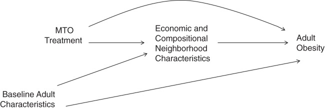
Directed acyclic graph for the empirical example. We hypothesized that the treatment effects of the Moving to Opportunity (MTO) intervention on adult obesity would be mediated by economic and compositional neighborhood characteristics, conditional on potential preexposure covariates.

Table 1.

Testing of Mediation of the Effects of Moving to Opportunity^a Housing Voucher Intervention (vs. Remaining in Public Housing (Control Group)) on Adult Obesity Prevalence in 2002 Using Inverse Odds Weighting^b

Effect of Treatment on Obesityc	Mediator(s)d
	All 4 Census Factors			Economic Factor Only
	RR	95% CI	P Value	RR	95% CI	P Value
Indirect effect	0.95	0.89, 1.02	0.15	0.96	0.92, 1.00	0.04
Direct effect	0.95	0.86, 1.06	0.36	0.95	0.87, 1.04	0.25
Total effect	0.91	0.84, 0.98	0.02	0.91	0.84, 0.98	0.02

Abbreviations: CI, confidence interval; RR, relative risk.

^a n = 3,401 adult household heads in the Moving to Opportunity experiment (1994–2002).

^b Census tract data (Census 2000) were linked to 1997 census tract locations of the residential addresses of Moving to Opportunity participants. In binary treatment models, the Section 8 housing voucher group was compared with public housing controls. The Section 8 voucher group combined the 2 originally randomized groups: the low-poverty neighborhood Section 8 group and the regular Section 8 group.

^c Covariates included adult baseline characteristics such as study site, age, sex, race, ethnicity, marital status, employment status, receipt of welfare, education, school enrollment, no teens in the household at baseline, household member with a disability, having lived in the baseline neighborhood for 5 or more years, feeling very unsafe in the neighborhood, and having moved more than 3 times prior to baseline.

^d Four mediators were derived from exploratory factor analysis: 1) an economic factor (median family income, percentage of people aged ≥25 years with a college degree, percentage of owner-occupied housing units, percentage of female-headed households with children, percentage of people aged ≥25 years with less than a high school diploma, percent unemployed among persons aged ≥16 years in the civilian labor force, percentage of households receiving public assistance, percentage of people in poverty); 2) a business factor (number of businesses, annual payroll, number of employees); 3) a minority composition factor (percent non-Hispanic black, percent Hispanic, percent foreign-born); and 4) a minority males and minority adults factor (percentage of the population who were minority males aged ≥16 years among employed civilians, percentage of minority males aged 10–19 years, percentage of minority adults aged ≥25 years).

IORW and IOW mediation analyses were implemented in Stata/SE 11 (StataCorp LP, College Station, Texas), with bootstrapped (1,000 iterations) standard errors. The validity of bootstrap-based inference relies on one's ability to respect the original study design in the process of generating bootstrap samples. This process can be quite involved in the context of survey weights (43), and therefore it was forgone in the current illustration, in favor of a simpler analysis in which we accounted for possible selection bias by adjusting for a fairly extensive set of prerandomization covariates in all regression models. We confirmed that our strategy was indeed appropriate by informally comparing point estimates without and with MTO survey weights (Table 1 vs. Web Table 1) to ensure that conclusions were consistent. Results were qualitatively similar, though indirect effects were somewhat attenuated without the MTO survey weights.

Web Appendix 3 contains sample Stata code for implementing IOW and the nonparametric bootstrap. Web Appendix 4 contains Stata code for IOW combined with bootstrapping of multiply imputed data (44). Researchers utilizing multiple mediators may adopt an imputation strategy to preserve sample size. Under a missing-at-random assumption, multiple imputation may allow for more precise and less biased estimates than a complete case analysis (45). The Stata code included in Web Appendix 3 implements a procedure called multiple imputation by chained equations (MICE), which produces imputed data sets by utilizing a series of imputation models, 1 model for each variable with missing data (44). Rubin's rule was used to combine estimates across imputed data sets (44, 46). Web Appendix 5 provides Stata code for constructing IORW weights (instead of IOW-stabilized weights). In our example, IOW and IORW estimates were almost identical, but IOW standard errors were smaller, given stabilization, as anticipated.

Results from the empirical example

Among 3,401 MTO adult household heads in our analytical sample (i.e., with nonmissing values on BMI, covariates, and mediators), the MTO voucher program had a significant protective total effect against obesity (11% risk reduction) in comparison with controls remaining in public housing (relative risk = 0.89, 95% confidence interval (CI): 0.89, 0.98). Obesity prevalence in the control group was 46.8% as compared with 42.3% for combined treatment groups. Using IOW to test mediation, the 4 factor scores, corresponding to neighborhood characteristics in 1997 (0–3 years following baseline and random assignment), accounted for 49% of the total effect (Table 1), suggesting that changes in census tract characteristics induced by the MTO intervention substantially mediated MTO treatment effects on obesity. When all 4 factors were entered together, the relative risk for the indirect effect was 0.95 (95% CI: 0.89, 1.02; P = 0.15) (Table 1). When only the economic factor was included, the relative risk for the indirect effect was 0.96 (95% CI: 0.92, 1.00; P = 0.04), suggesting that this pathway accounted for most of the indirect effect.

Additionally, using continuous BMI as the outcome variable (rather than the dichotomous obesity variable), we found that MTO treatment was associated with approximately a 1-unit decrease in BMI (total effect: −0.91; P = 0.001). The 4 factors together mediated 56% of the total effect (indirect effect: −0.50; P = 0.12), although results were once again driven by economic and business characteristics (indirect effect: −0.58, P = 0.11). Thus, our empirical example suggests that the effect of MTO treatment on adult obesity was partially mediated through structural neighborhood characteristics. In particular, we found that economic characteristics of census tracts, not the demographic composition of neighborhoods, mattered for adult obesity and the BMI status of adults 4–7 years after random assignment to the MTO housing choice voucher program.

The IORW method relies upon the investigator to select mediator variables that s/he thinks are important intermediates between the exposure and the outcome. An incredible strength of the IORW method is that it can accommodate multiple mediators, unlike many other mediation methods. However, including many mediators, especially in a small data set, may produce unreliable or unstable weights or effect estimates. The same is true of covariates. The tradeoff is that if important covariates are omitted, estimates may be biased, since covariates are included to control for confounding of the exposure, mediator, and outcome relationships.

Because of randomization, total effects of the intervention could, in principle, be evaluated without concerns about confounding bias. However, mediating factors are not randomized, and therefore, despite efforts to account for baseline confounders, unobserved confounding cannot be ruled out with certainty. In a sensitivity analysis, we adjusted for additional available preexposure covariates (a total of 28 covariates) and found very comparable indirect effects.

As we noted previously, we additionally assume, as do other mediation methods (9, 12, 47, 48), that there are no confounders of the mediator-outcome relationship that are affected by the exposure. This assumption, in essence, requires that pathways between the exposure and mediator do not also affect the outcome (4). When this assumption does not hold, natural indirect and direct effects, in general, cannot be identified—although there are exceptions (27, 29, 49, 50), including the case where there is no individual-level additive effect of interaction between the exposure and mediator on the outcome, an assumption that cannot be confirmed empirically (51). One practical implication is that the closer in time the mediator is measured as compared with the exposure, the less likely this assumption is to be violated. To minimize potential violation of this assumption, in our empirical example, our mediators were linked to time points closer to baseline than to outcome measurements; for example, census tract characteristics were linked to MTO participants' 1997 locations (0–3 years following random assignment). In sensitivity analyses, we restricted the analytical sample to persons with 1997 study entry dates (n = 1,099), and thereby the mediator was modeled within 1 year of random assignment. Indirect effects were robust to this restriction, and indeed hypothesized mediator variables accounted for an even larger percentage of total effects, compared with results from the entire sample.

Additionally, in sensitivity analyses we assessed the amount of confounding induced by unobserved variables that could potentially bias our observed finding, by applying methods recommended by Tchetgen Tchetgen and Shpitser (6, 17). Briefly, the sensitivity analysis quantifies the possible confounding bias present in the direct effect (and the indirect effect) given measured confounders, by offsetting the observed outcome by a value encoded in a selection bias function. The specific methods used to calculate the selection bias function and the corresponding outcome offset are detailed in Web Appendix 2, and the ranges of direct and indirect effects are plotted across levels of our chosen sensitivity parameter (λ(c)), which captures, for a binary mediator, the following counterfactual difference: λ(c) = 𝔼(Y_e=1,m|E = 1, M = 1, C) − 𝔼(Y_e=1,m|E = 1, M = 0, C).

Clearly, λ(C) is zero for all levels of C only if M is unconfounded given C; otherwise, λ(C) captures the extent to which confounding may lead to differences in the average potential BMI (Y_e=1,m) under an intervention moving people to a low-poverty neighborhood (M = 1) with a voucher (E = 1), comparing persons who were observed to have moved with the help of a voucher with persons who failed to move despite receiving the voucher. A positive value of λ(C) indicates that persons with greater BMI were more likely to adhere to the intervention, while a negative value of λ(C) indicates the opposite. Thus, by varying λ(C) one can obtain a sensitivity analysis for confounding of the mediator (6, 17). We implemented the approach in the MTO data upon making the simplifying assumption that λ(C) = λ does not depend on C. The direct effect plot (Web Figure 1) indicates very little bias in the direct effect; the direct effect coefficient remains consistent (ranging from 0.195 to 0.219) and nonsignificant. The indirect effect coefficient ranges from −0.930 to −1.306; however, the significance level is more sensitive to bias. Specifically, the indirect effect coefficient has P < 0.1 when λ ranges from −0.3 to 1.5, but the indirect effect has P > 0.1 when λ ranges from −1.5 to −0.4. This suggests that the indirect effect may be overestimated due to confounding bias for values of λ below −0.4—that is, if the potential BMI (under the active intervention) of persons more likely to adhere to the intervention was in actuality at least 0.4 units lower than that of persons less likely to adhere.

Nonlinearities in the IORW model can be incorporated through variable specification (e.g., including polynomial terms for some mediators in the regression model). To simplify the exposition, we considered only linear main effects for the application.

CONCLUSION

In this paper we have demonstrated the utility and advantages of IORW mediation over the use of other methods, have presented an empirical example, and have provided statistical code for its implementation. Testing of mediation is necessary to understand the active components of exposures and of interventions for improving population health, and it can be facilitated by easier implementation of such methods.

REFERENCES

- 1.Imai K, Keele L, Tingley D. A general approach to causal mediation analysis. Psychol Methods. 2010;15(4):309–334. doi: 10.1037/a0020761. [DOI] [PubMed] [Google Scholar]
- 2.Pearl J. Direct and indirect effects; Proceedings of the Seventeenth Conference on Uncertainty in Artificial Intelligence (UAI-2001); San Francisco, CA: Morgan Kaufmann Publishers, Inc.; 2001. pp. 411–420. [Google Scholar]
- 3.Robins JM, Greenland S. Identifiability and exchangeability for direct and indirect effects. Epidemiology. 1992;3(2):143–155. doi: 10.1097/00001648-199203000-00013. [DOI] [PubMed] [Google Scholar]
- 4.VanderWeele TJ, Vansteelandt S. Conceptual issues concerning mediation, interventions and composition. Stat Interface. 2009;2(4):457–468. [Google Scholar]
- 5.VanderWeele TJ, Vansteelandt S. Odds ratios for mediation analysis for a dichotomous outcome. Am J Epidemiol. 2010;172(12):1339–1348. doi: 10.1093/aje/kwq332. [DOI] [PMC free article] [PubMed] [Google Scholar]
- 6.Tchetgen Tchetgen EJ, Shpitser I. Semiparametric Estimation of Models for Natural Direct and Indirect Effects. Boston, MA: Harvard University; 2011. (Harvard University Biostatistics Working Paper Series). http://biostats.bepress.com/harvardbiostat/paper129 . Accessed April 15, 2013. [Google Scholar]
- 7.Pearl J. The causal mediation formula—a guide to the assessment of pathways and mechanisms. Prev Sci. 2012;13(4):426–436. doi: 10.1007/s11121-011-0270-1. [DOI] [PubMed] [Google Scholar]
- 8.Tchetgen Tchetgen EJ. Inverse odds ratio-weighted estimation for causal mediation analysis. Stat Med. 2013;32(26):4567–4580. doi: 10.1002/sim.5864. [DOI] [PMC free article] [PubMed] [Google Scholar]
- 9.Valeri L, VanderWeele TJ. Mediation analysis allowing for exposure-mediator interactions and causal interpretation: theoretical assumptions and implementation with SAS and SPSS macros. Psychol Methods. 2013;18(2):137–150. doi: 10.1037/a0031034. [DOI] [PMC free article] [PubMed] [Google Scholar]
- 10.Imai K, Keele L, Tingley D, et al. Causal mediation analysis using R. In: Vinod HD, editor. Advances in Social Science Research Using R. New York, NY: Springer Publishing Company; 2010. pp. 129–154. [Google Scholar]
- 11.Lange T, Vansteelandt S, Bekaert M. A simple unified approach for estimating natural direct and indirect effects. Am J Epidemiol. 2012;176(3):190–195. doi: 10.1093/aje/kwr525. [DOI] [PubMed] [Google Scholar]
- 12.Lange T, Hansen JV. Direct and indirect effects in a survival context. Epidemiology. 2011;22(4):575–581. doi: 10.1097/EDE.0b013e31821c680c. [DOI] [PubMed] [Google Scholar]
- 13.VanderWeele TJ. Marginal structural models for the estimation of direct and indirect effects. Epidemiology. 2009;20(1):18–26. doi: 10.1097/EDE.0b013e31818f69ce. [DOI] [PubMed] [Google Scholar]
- 14.van der Laan MJ, Petersen ML. Direct effect models. Int J Biostat. 2008;4(1):Article 23. doi: 10.2202/1557-4679.1064. [DOI] [PubMed] [Google Scholar]
- 15.Albert JM. Distribution-free mediation analysis for nonlinear models with confounding. Epidemiology. 2012;23(6):879–888. doi: 10.1097/EDE.0b013e31826c2bb9. [DOI] [PMC free article] [PubMed] [Google Scholar]
- 16.Zheng W, van der Laan MJ. Targeted maximum likelihood estimation of natural direct effects. Int J Biostat. 2012;8(1):Article 3. doi: 10.2202/1557-4679.1361. [DOI] [PMC free article] [PubMed] [Google Scholar]
- 17.Tchetgen Tchetgen EJ, Shpitser I. Semiparametric theory for causal mediation analysis: efficiency bounds, multiple robustness and sensitivity analysis. Ann Stat. 2012;40(3):1816–1845. doi: 10.1214/12-AOS990. [DOI] [PMC free article] [PubMed] [Google Scholar]
- 18.Tchetgen Tchetgen EJ. On causal mediation analysis with a survival outcome. Int J Biostat. 2011;7(1):1–38. doi: 10.2202/1557-4679.1351. [DOI] [PMC free article] [PubMed] [Google Scholar]
- 19.Vansteelandt S, Bekaert M, Lange T. Imputation strategies for the estimation of natural direct and indirect effects. Epidemiol Methods. 2012;1(1):131–158. doi: 10.1093/aje/kwr525. [DOI] [PubMed] [Google Scholar]
- 20.Baron RM, Kenny DA. The moderator-mediator variable distinction in social psychological research: conceptual, strategic, and statistical considerations. J Pers Soc Psychol. 1986;51(6):1173–1182. doi: 10.1037//0022-3514.51.6.1173. [DOI] [PubMed] [Google Scholar]
- 21.VanderWeele TJ, Vansteelandt S. Mediation analysis with multiple mediators. Epidemiol Methods. 2013;2(1):95–115. doi: 10.1515/em-2012-0010. [DOI] [PMC free article] [PubMed] [Google Scholar]
- 22.Lange T, Rasmussen M, Thygesen LC. Assessing natural direct and indirect effects through multiple pathways. Am J Epidemiol. 2014;179(4):513–518. doi: 10.1093/aje/kwt270. [DOI] [PubMed] [Google Scholar]
- 23.Jong G, Nomi T. Weighting methods for assessing policy effects mediated by peer change. J Res Educ Eff. 2013;5(3):261–289. [Google Scholar]
- 24.Greenland S. Tests for interaction in epidemiologic studies: a review and a study of power. Stat Med. 1983;2(2):243–251. doi: 10.1002/sim.4780020219. [DOI] [PubMed] [Google Scholar]
- 25.Marshall SW. Power for tests of interaction: effect of raising the Type I error rate. Epidemiol Perspect Innov. 2007;4:4. doi: 10.1186/1742-5573-4-4. [DOI] [PMC free article] [PubMed] [Google Scholar]
- 26.Robins JM, Richardson TS. Alternative graphical causal models and the identification of direct effects. In: Shrout PE, Keyes KM, Orstein K, editors. Causality and Psychopathology: Finding the Determinants of Disorders and Their Cures. New York, NY: Oxford University Press; 2011. pp. 103–158. [Google Scholar]
- 27.Tchetgen Tchetgen EJ, VanderWeele TJ. Identification of natural direct effects when a confounder of the mediator is directly affected by exposure. Epidemiology. 2014;25(2):282–291. doi: 10.1097/EDE.0000000000000054. [DOI] [PMC free article] [PubMed] [Google Scholar]
- 28.VanderWeele TJ. Bias formulas for sensitivity analysis for direct and indirect effects. Epidemiology. 2010;21(4):540–551. doi: 10.1097/EDE.0b013e3181df191c. [DOI] [PMC free article] [PubMed] [Google Scholar]
- 29.Imai K, Keele L, Yamamoto T. Identification, inference and sensitivity analysis for causal mediation effects. Stat Sci. 2010;25(1):51–71. [Google Scholar]
- 30.Tchetgen Tchetgen EJ. On the interpretation, robustness, and power of varieties of case-only tests of gene-environment interaction. Am J Epidemiol. 2010;172(12):1335–1338. doi: 10.1093/aje/kwq359. [DOI] [PMC free article] [PubMed] [Google Scholar]
- 31.Imai K, Keele L, Yamamoto T. Identification, inference and sensitivity analysis for causal mediation effects. Stat Sci. 2009;25(1):51–71. [Google Scholar]
- 32.Preacher KJ, Hayes AF. SPSS and SAS procedures for estimating indirect effects in simple mediation models. Behav Res Methods Instrum Comput. 2004;36(4):717–731. doi: 10.3758/bf03206553. [DOI] [PubMed] [Google Scholar]
- 33.Muthén B. Applications of Causally Defined Direct and Indirect Effects in Mediation Analysis Using SEM in Mplus. Los Angeles, CA: Muthén and Muthén; 2011. (Working paper) http://www.statmodel.com/download/causalmediation.pdf. Accessed April 2, 2013. [Google Scholar]
- 34.Tchetgen Tchetgen EJ, Robins JM, Rotnitzky A. On doubly robust estimation in a semiparametric odds ratio model. Biometrika. 2010;97(1):171–180. doi: 10.1093/biomet/asp062. [DOI] [PMC free article] [PubMed] [Google Scholar]
- 35.Orr L. Moving to Opportunity (MTO) for Fair Housing Demonstration: Interim Impacts Evaluation, Tier 1 Restricted Access Data, 1994–2001 [United States] (ICPSR 31661) Ann Arbor, MI: Inter-University Consortium for Political and Social Research; 2011. http://www.icpsr.umich.edu/icpsrweb/ICPSR/studies/31661 . Accessed January 12, 2013. [Google Scholar]
- 36.Goering J, Kraft J, Feins J, et al. Moving to Opportunity for Fair Housing Demonstration Program: Current Status and Initial Findings. Washington, DC: Office of Policy Development and Research, US Department of Housing and Urban Development; 1999. [Google Scholar]
- 37.Osypuk TL, Tchetgen Tchetgen EJ, Acevedo-Garcia D, et al. Differential mental health effects of neighborhood relocation among youth in vulnerable families: results from a randomized trial. Arch Gen Psychiatry. 2012;69(12):1284–1294. doi: 10.1001/archgenpsychiatry.2012.449. [DOI] [PMC free article] [PubMed] [Google Scholar]
- 38.DeVellis RF. Scale Development: Theory and Applications. 1st ed. Newbury Park, CA: Sage Publications; 1991. Factor analytic strategies; pp. 91–109. (Applied Social Research Methods, vol. 26) [Google Scholar]
- 39.Elmståhl S, Gullberg B. Bias in diet assessment methods—consequences of collinearity and measurement errors on power and observed relative risks. Int J Epidemiol. 1997;26(5):1071–1079. doi: 10.1093/ije/26.5.1071. [DOI] [PubMed] [Google Scholar]
- 40.Hosmer DW, Lemeshow S. Applied Logistic Regression, Second Edition. New York, NY: John Wiley & Sons, Inc.; 2000. [Google Scholar]
- 41.Zou G. A modified Poisson regression approach to prospective studies with binary data. Am J Epidemiol. 2004;159(7):702–706. doi: 10.1093/aje/kwh090. [DOI] [PubMed] [Google Scholar]
- 42.Orr L, Feins JD, Jacob R, et al. Appendix B: samples and analysis methods. In:Moving to Opportunity for Fair Housing Demonstration Program: Interim Impacts Evaluation. Washington, DC: US Office of Policy Development and Research, Department of Housing and Urban Development; 2003. pp. B1–B31. [Google Scholar]
- 43.Shao J. Impact of the bootstrap on sample surveys. Stat Sci. 2003;18(2):191–198. [Google Scholar]
- 44.Royston P, White IR. Multiple imputation by chained equations (MICE): implementation in Stata. J Stat Softw. 2011;45(4):1–20. [Google Scholar]
- 45.White IR, Carlin JB. Bias and efficiency of multiple imputation compared with complete-case analysis for missing covariate values. Stat Med. 2010;29(28):2920–2931. doi: 10.1002/sim.3944. [DOI] [PubMed] [Google Scholar]
- 46.Little RJA, Rubin DB. Statistical Analysis with Missing Data. 2nd ed. New York, NY: John Wiley & Sons, Inc.; 2002. [Google Scholar]
- 47.Vansteelandt S, Lange C. Causation and causal inference for genetic effects. Hum Genet. 2012;131(10):1665–1676. doi: 10.1007/s00439-012-1208-9. [DOI] [PubMed] [Google Scholar]
- 48.Cole SR, Hernán MA. Fallibility in estimating direct effects. Int J Epidemiol. 2002;31(1):163–165. doi: 10.1093/ije/31.1.163. [DOI] [PubMed] [Google Scholar]
- 49.Petersen ML, Sinisi SE, van der Laan MJ. Estimation of direct causal effects. Epidemiology. 2006;17(3):276–284. doi: 10.1097/01.ede.0000208475.99429.2d. [DOI] [PubMed] [Google Scholar]
- 50.Hafeman DM, VanderWeele TJ. Alternative assumptions for the identification of direct and indirect effects. Epidemiology. 2011;22(6):753–764. doi: 10.1097/EDE.0b013e3181c311b2. [DOI] [PubMed] [Google Scholar]
- 51.Robins JM. Semantics of causal DAG models and the identification of direct and indirect effects. In: Green P, Hjort NL, Richardson S, editors. Highly Structured Stochastic Systems. New York, NY: Oxford University Press; 2003. pp. 70–81. [Google Scholar]
Associated Data
This section collects any data citations, data availability statements, or supplementary materials included in this article.