The DIADEM Data Sets: Representative Light Microscopy Images of Neuronal Morphology to Advance Automation of Digital Reconstructions

Abstract

The comprehensive characterization of neuronal morphology requires tracing extensive axonal and dendritic arbors imaged with light microscopy into digital reconstructions. Considerable effort is ongoing to automate this greatly labor-intensive and currently rate-determining process. Experimental data in the form of manually traced digital reconstructions and corresponding image stacks play a vital role in developing increasingly more powerful reconstruction algorithms. The DIADEM challenge (short for DIgital reconstruction of Axonal and DEndritic Morphology) successfully stimulated progress in this area selecting six data set collections from different animal species, brain regions, neuron types, and visualization methods. The original research projects that provided these data are representative of the diverse scientific questions addressed in this field. At the same time, these data provide a benchmark for the types of demands automated software must meet to achieve the quality of manual reconstructions while minimizing human involvement. The DIADEM data underwent extensive curation, including quality control, metadata annotation, and format standardization, to focus the challenge on the most substantial technical obstacles. This data set package is now freely released (http://diademchallenge.org) to train, test, and aid development of automated reconstruction algorithms.

Introduction

Reconstruction of neuronal morphology provides a popular and valuable approach to quantifying axonal and dendritic structure. Digital tracing permanently stores relevant morphometric information in compact and easily shared files. These data can be re-analyzed in future research projects, often in ways not envisioned in the original experimental design (Ascoli et al., 2009; Fares and Stepanyants, 2009; Torben-Nielsen and Stiefel, 2009; Volman et al., 2009; Snider et al., 2010).

By far the most common digital reconstruction approach involves tracing neurons manually where an operator interacts with computer software to individually create and interconnect each trace point. Depending on the size, complexity, and number of arbors traced, manual reconstructions can take up to several months to finish. As histological and imaging methods advance, studies will increasingly benefit from the opportunity to reconstruct greater numbers of neurons. The desire to automate this process is progressively becoming a need, as current labor-intensive reconstruction methods continue to limit neuroscientific productivity.

A few software products for automatically reconstructing neuronal morphology have already been developed both in the commercial sector, such as the AutoNeuron extension module for Neurolucida (MBF Bioscience, Williston, VT) or Imaris Filament Tracer (Bitplane, Zurich, Switzerland) and in academia, including V3D (Peng et al., 2010), ORION (Losavio et al., 2008), and NeuronStudio (Rodriguez et al., 2009). However, their infrequent application and the intense ongoing activity for further development (Donohue and Ascoli, 2011) suggest that these existing options have limited utility. Typically, these programs perform well with simple neuronal trees or individual data sets, but require extensive human intervention for complex arbors or diverse experimental data. The purpose of the 2010 DIADEM (DIgital reconstruction of Axonal and DEndritic Morphology) challenge was to motivate advances in automated reconstruction methods with the hope of developing algorithms that tackle the rate-limiting issues faced in the reconstruction process. Specifically, automated methods must be capable of producing accurate reconstructions in only a fraction of the labor time required to produce manual reconstructions, regardless of how human interaction time is spent (e.g. tuning the automated reconstruction program, fixing trace points, etc.).

A large variety of histological preparations and imaging technologies are in use today. Laboratories interested in reconstructing neuronal trees typically select among confocal, 2- or multi-photon, and bright field microscopy depending on instrument availability, resolution requirements, and a broad choice of neuronal labeling method. An additional dimension of variability exists in animal species, brain regions, and neuronal type. Axons and dendrites vary widely in size and projection both within and across neuronal classes. For instance, CA3 pyramidal axon arbors can project to the majority of the hippocampus with a total length of 500 mm (Wittner et al., 2007), while dentate granule cell axons have limited span and average total lengths of ~8 mm (Buckmaster and Dudek, 1999). Altogether, these variables produce a wide array of challenges that automated reconstruction programs must face in order to be broadly applicable. Thus, in order to confront such challenges, a representative sample of data from a variety of labs was incorporated into DIADEM. This review describes common and unique aspects of each of the DIADEM data sets including why they were originally acquired, how they were processed and are distributed, and the types of demands these data sets provide for automating reconstructions.

The DIADEM Data Sets

Six laboratories provided data that together encompassed a variety of animal species, brain regions, cell and arbor types, histology, microscopy, and research goals (Table 1). The DIADEM data sets were carefully selected to represent the scientific problems addressed with reconstructions and the demands automated algorithms must overcome.

Table 1.

Data set materials and methods

Nervous system region	Cerebellar cortex	Antennal lobe	Neocortex (layer 1)	Peripheral neuromuscular	Hippocampal CA3	Primary visual cortex (layer 6)
Fiber type	Climbing fiber axon terminal	Axon	Axon	α-motoneuron axonal arbor	Interneuron axon/dendrite	Simple cell axon/dendrite
Lab	Sugihara, Ascoli	Jefferis, Luo	De Paola	Lichtman	Barrionuevo	Hirsch
Species	Rat	Drosophila	Mouse	Mouse	Rat	Cat
Strain	Long-Evans	single cell MARCM1	C57BL/6 2	C57BL/6 3	Sprague-Dawley	N/A
Labeling	Biotinylated Dextran Amine	Membrane- targeted GFP	Membrane-targeted GFP	Cytoplasmic YFP	Biocytin	Biocytin
Digital tracing	Neurolucida	Neurolucida, hxskeletonize	Neurolucida	Reconstruct, NeuronJ	Neurolucida	Neurolucida
Microscopy	Transmitted light brightfield	Confocal	in vivo 2-photon laser scanning	Confocal	Transmitted light brightfield	Transmitted light brightfield
Objective lens	100x oil, 1.3 NA, 2.0x zoom	40x oil, 1.3 NA, 1.5x zoom	40x water, 0.8 NA	63x oil, 1.4 NA	100x oil, 1.4 NA, 1.6x zoom	63x oil, 1.4 NA

¹Transgene GAL4-GH146 UAS-mCD8-GFP

²Transgene Thy1 (line 15)

³Transgene Thy1-YFP-16

This section briefly describes the original scientific purposes for which each of these data sets were acquired, as well as the experimental methods used by each of the data set providers, starting with general acquisition steps that apply to all data sets. The magnitude of labor required to produce the manual reconstructions is emphasized along with future research goals that will require reconstruction automation. The next section explains the process undertaken to organize and distribute these data to aid development, evaluation, and extension of automated reconstruction algorithms.

General Data Set Acquisition Steps

Each data set consisted of manually traced digital reconstructions and image stacks of the corresponding tissue. To obtain the image stacks, a portion of neuronal structures are labeled in brain tissue and then mounted on microscope slides or imaged in situ in the case of the in vivo neocortical projection data set. The slide is viewed through a microscope equipped with a digital camera or, for confocal and two-photon microscopy, a photomultiplier tube (PMT). The camera can produce a live feed transferred to a computer where specialized software is used to trace neural structures without storing imaging data. Alternatively, a series of high resolution images of a region of interest taken while changing the focus level provides the ability to visualize the entire 3D neuronal structure. These images are stored and subsequently loaded into digital tracing software. Reconstructions consist of a connected series of individual points that are traced over the image stack structure they are intended to represent. Each point is stored with a unique identifier, its arbor type (e.g. axon or dendrite), position in X, Y, and Z, branch thickness, and the previous (i.e. parent) trace point to which it connects (Fig. 1A).

Fig. 1.

(A) Portion of an SWC reconstruction file. Each row represents one trace point with a unique ID, arbor type tag, X, Y and Z position, radius, and parent ID. (B through D) Training (cyan), Qualifier (yellow) and Final (red) Round climbing fiber manual reconstructions. Reconstructions slightly offset from image stacks for better visualization.

Cerebellar Climbing Fiber Data Set

Climbing fibers are axon terminals of inferior olive neurons that provide powerful excitatory input to Purkinje cells in the cerebellar cortex. This data set was originally acquired to analyze in detail climbing fiber morphological properties and anatomical relationships from the axonal origin in the inferior olive through the terminations in the cerebellar cortex (Sugihara et al., 1999). For this purpose, biotinylated dextran amine (BDA) was injected in the inferior olive of adult rats to label entire olivocerebellar axonal trajectories. BDA is one of the most efficient anterograde tracers available (Sugihara, 2011), allowing for direct observation and photomicrographic documentation by standard light microscopy (Fig. 1).

It was found that almost all olivocerebellar axons entered the cerebellum via the contralateral inferior cerebellar peduncle. On average, seven climbing fibers arose from each inferior olive axon. It was also confirmed that climbing fibers typically synapse with Purkinje cells in a one-to-one relationship. Since the Purkinje cell dendritic tree is organized within a semi-parasagittal (longitudinal) plane, the terminal arbor of the climbing fiber is also organized within the same semi-parasagittal plane. Although previous reports suggested climbing fibers only synapsed on Purkinje cell dendrites, some proportion of their branches contacted the Purkinje cell body. An unreported climbing fiber branch type we classified as ‘transverse branchlets’ was discovered that traveled in an orthogonal (transverse) direction to the terminal arbor of the climbing fiber for a short distance. Transverse branchlets and evidence of branch terminations contacting counter-stained interneuronal cell bodies suggest that the climbing fiber may contact other cells beyond the underlying Purkinje cell.

A single cerebellar climbing fiber can take 3–4 hours to trace two-dimensionally with a camera lucida system. The planar organization of the arbor of a climbing fiber often allows it to be localized within a single microtome section of the cerebellum (50–80 μm thick) if the section is cut in parallel to the plane of the arbor, favoring automation. Manual 3D climbing fiber reconstructions can take 6 to 24 hours full time, with an average estimated at 14 hours. Tracing entire olivocerebellar single axons from serial sections using a semi-3D method (using the section rank multiplied by the section thickness as the z-coordinate) takes about 20 days at 6 hours per day or 120 hours.

Although climbing fibers are distributed throughout the cerebellar cortex, the cerebellar cortex has transverse (lobular) and longitudinal compartmentalization. The latter is related to different levels of expression of several molecules in subpopulation of Purkinje cells. This organization reflects the functional localization of the cerebellum. It would be valuable to examine potential climbing fiber morphological subsets by cerebellar regional location. The relation of climbing fiber morphology to cerebellar compartmentalization will be studied better with automated than with manual tracing, since a large sample would be required. Moreover, the morphology of climbing fibers is formed in early postnatal days. Several methods for artificial alteration of cerebellar development, including genetic manipulation, cause different kinds of malformation of climbing fibers as well as of other neuronal components of the cerebellar cortex. Quantitative data obtained by automated tracing software may be particularly useful to assess the climbing fiber morphogenetic process.

Olfactory Projection Fiber Data Set

These data came from two studies of the organization of the central olfactory system in Drosophila (Marin et al., 2002; Jefferis et al., 2007). Previous work had shown that as in vertebrates the axons of olfactory sensory neurons expressing the same odorant receptor converge at stereotyped glomeruli in the first relay in the brain, called the antennal lobe in insects (Gao et al., 2000; Vosshall et al., 2000). However the anatomical logic of the second order neurons, called projection neurons, was not clear. We used a genetic labeling technique known as MARCM (Lee and Luo, 1999) to address this problem. The target population contained about 90 genetically defined projection neurons (out of an estimated total of 150). MARCM allowed us to generate many brains containing single green fluorescent protein (GFP) labeled neurons. We imaged brains using whole mount confocal microscopy and traced the neurons (Fig. 2) using either manual or semi-automatic approaches, such as the Amira (Mercury Computer Systems, Inc., Chelmsford, MA) extension module hxskeletonize (Evers et al., 2005). By co-registering different sample brains we were able to build up a full 3D atlas (Jefferis et al., 2007).

Fig. 2.

(A) Olfactory projection neuron tree sample. Red square encompasses region in (B), which shows the topological complexity of the terminal region. Reconstruction slightly offset from image stacks for better visualization.

This work demonstrated a highly stereotyped spatial map of olfactory information in one higher olfactory center in the fly brain (the lateral horn). This map is much more distributed than that in the first olfactory relay; anatomical convergence and divergence likely allow integration of information originating from different glomeruli. Mapping projects of this sort could be used to provide a full 3D atlas of the estimated 100,000 neurons in the fly brain. Tackling a project of such scale would require increased throughput of confocal imaging of brains and genetic labeling schemes that allow many neurons to be distinctly labeled in the same brain. Progress has been made on both of these points. However, the typical time for manual tracing of the relatively simple neurons in our data set was about 20 minutes, and many neurons are much more complex, so tracing remains a major bottleneck.

Neocortical Layer 1 Axon Data Set

Acquisition of this data set was originally motivated by the study of the cellular and circuit mechanisms of experience-dependent plasticity and repair (Canty and De Paola, 2011). To understand the full capacity of reorganization of the adult mammalian brain, neurons, their synapses and activity patterns therein need to be studied in situ over extended periods of time. Due to technical challenges in tracking defined axonal pathways in living animals little is known about the regulation of axonal plasticity in the adult brain. Axons arborize extensively in Layer 1 of the neocortex and form a remarkably dense and poorly characterized network. Axons can be effectively labeled, visualized and imaged in vivo using a membrane-bound form of GFP expressed in subsets of neurons (Thy-1 mouse line 15, De Paola et al., 2003) and 2-photon microscopy (De Paola et al., 2006). At the moment the analysis of axonal morphology and dynamics from 2-photon fluorescent image stacks heavily relies on manual reconstructions and is both arduous and extremely time-consuming. Each isolated 150×150×50 μm stack (x-y-z, L1 axon data set) took several hours to trace, excluding proofreading. To reconstruct by hand all Thy1-GFP labeled axons in the first two cortical layers of a slice of the mouse cortex, a volume of approximately 10×10×0.15 mm, from just one time point, would take several years of work, excluding the mapping of synaptic sites. The value of accurate and efficient automated reconstruction algorithms will be amplified when applied to the same region of circuitry over several time points, enabling identification and quantification of any ensuing length or synaptic rearrangements.

Data for the Qualifier and Training rounds (Fig. 3) came from the whole mount fixed brain of a 2 month-old animal. The left hemisphere was imaged approximately in the motor cortex, using a Prairie ULTIMA 2-photon system (Prairie Technologies) controlled via Prairie view software. Nine overlapping stacks of various thickness (range: 33–64 μm) were captured, with approximate 15 μm overlap in x-y. Data for the Final round was imaged from a 4-month old mouse through a viewing window (Holtmaat et al., 2009) under ketamine/xylazine anesthesia, using the same acquisition settings as for the other rounds (Table 1), except having 10 overlapping tiles (z-thickness range: 50–88 μm). This is the only DIADEM data set acquired in a living animal. This means that movement artifacts due to the animal breathing and blood vessel contraction could make the automated reconstructions more challenging, especially when repeated over consecutive imaging sessions.

Fig. 3.

Example neocortical axon trees (colored separately) overlap and project over the same image stack tiles. Branch radius added for better visualization.

Neuromuscular Projection Fiber Data Set

The invertebrate nervous system is believed to be highly stereotyped due to tight genetic control; each neuron can often be identified by its specific structure and connectivity. To what extent such neuronal level stereotypy exists in mammals remains unclear. One major difficulty is to identify the exact counterpart of a mammalian neuron within a large population of similar cells for comparison. The mouse interscutularis muscle (a small ear muscle) is suitable to identify pairs of corresponding motor neurons with identical functions and compare their morphology and connections (Lu et al., 2009a). This peripheral neuromuscular circuit has several advantages. Adult motor axons can be readily resolved optically, and so are their synapses onto muscle fibers (the neuromuscular junction). Furthermore, in adult skeletal muscles, each muscle fiber is innervated by exactly one motor neuron. Therefore, the entire synapse-level wiring diagram, or “connectome,” can be obtained using optical microscopy. According to Henneman’s size principle (Henneman et al., 1965), motor neurons are recruited in a fixed order, which in turn corresponds to their motor unit sizes (the number of muscle fibers innervated by a motor neuron). Thus, neuronal counterparts can be identified by virtue of their motor unit size and rank within each connectome.

Production of this data set aimed at addressing these open issues using thy-1-YFP-16 transgenic mice (Feng et al., 2000), which express cytoplasmic yellow fluorescent protein (YFP) in all motor neurons. As optical sectioning is needed for tracing the trajectory of each axon, confocal microscopy was adopted for imaging (Fig. 4).

Fig. 4.

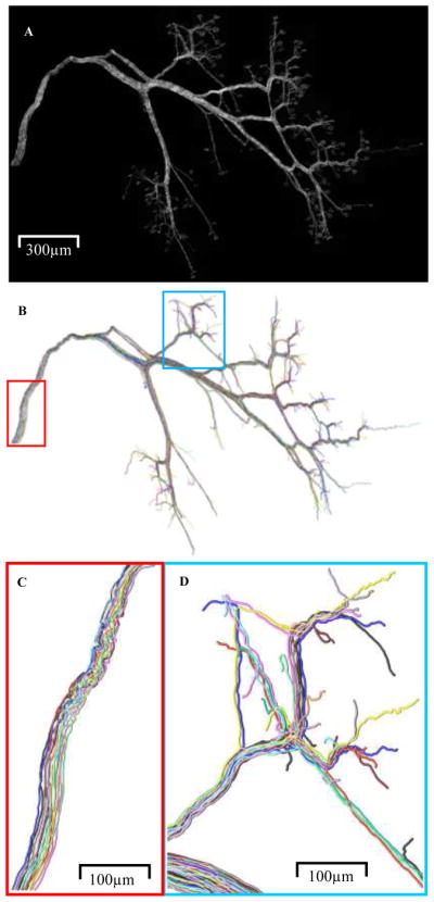
All 12 separately colored reconstructed neuromuscular projection fibers within the image stack (A) are shown (B). Zoomed-in regions show similarity in path near origin (C) and complex branch overlaps in terminal regions (D).

Reconstruction speed with Reconstruct (Fiala, 2005), the semi-automated reconstruction method employed in the muscle connectome analysis (Lu et al., 2009b), strongly depends on data quality and complexity. Under optimal conditions (i.e., crisp-clear images, with axonal profiles well segregated from their neighbors, and minimal user intervention required), the maximal speed is ~4 mm axon per hour. Under typical conditions (i.e., some axonal profiles not perfectly segregated; relatively large change in brightness; presence of intracellular organelles, etc., requiring user intervention), the speed is ~0.5 mm per hour. The total arbor length per axon ranges from ~5 mm to ~10 mm, and in each interscutularis muscle there are 12–16 axons. Thus the total time spent to reconstruct one muscle connectome was approximately 200–250 hrs. Subsequent concatenation of reconstructed axons from individual stacks into a single 2D montage in Photoshop (Adobe Systems, San Jose, CA) took 5–20 min per stack depending on the complexity of data, so the total time was 20–30 hrs. 2D re-tracing with NeuronJ (Meijering et al., 2004) to obtain the tree structure took about 10–20 min per axon or 2–3 hours in total.

Many further questions can be addressed by connectomic analysis of neuromuscular circuits. For instance, do axons “compartmentalize” their territories in large muscles? What is the organization of innervations when the circuit is still undergoing the postnatal re-organization known as synapse elimination? Answering these questions requires large numbers of data sets with more axons, more complicated innervation patterns, and less well-resolved structures. Analyzing such data sets manually would be extremely tedious and inefficient. It is expected that fully automated reconstruction algorithms, together with advances in labeling and imaging techniques, will facilitate such investigations.

Hippocampal CA3 Interneuron Data Set

The neuronal network in hippocampal area CA3 is composed of numerous subtypes of inhibitory interneurons which receive segregated inputs from different sources, including the commissural/association fibers from CA3 pyramidal cells, perforant path (PP) from entorhinal cortex layer 2, and mossy fibers (MF) from dentate gyrus granule cells. CA3 interneurons with soma in strata lacunosum-moleculare (L-M) and radiatum (R) provide a substantial fraction of dendritic and somatic feed-forward inhibition to CA3 pyramidal cells. The original purpose for the anatomical reconstruction of these interneurons was to assess the properties and mechanisms of temporal integration in R and L-M interneurons by taking advantage of the ability to activate independently convergent MF and PP inputs (Calixto et al., 2008).

Whole-cell recordings with biocytin-filled pipettes were obtained from the soma of putative interneurons localized 60–80 μm from the slice surface, and identified visually with infrared video microscopy and differential interference contrast optics. Advantages of biocytin are its high solubility in aqueous solutions and a small molecular weight, both of which facilitate injection using patch pipettes. In addition, biocytin is less expensive than alternatives such as Phaseolus Leucoagglutinin (PHA-L), and is easily transported by rat neurons to reveal the fine detail of axonal and dendritic processes. Biocytin-labeled interneurons were reconstructed with the Neurolucida tracing system from all sections containing the cell (Fig. 5).

Fig. 5.

(A) Complete CA3 hippocampal interneuron reconstruction. (B and C) Disconnected tree samples from two serial sections. Dendrites are either black or dark blue and axons are bright green, cyan, orange, and red. Colors besides bright green and black are used to match tree samples in (A) to (B and C).

Complete three-dimensional reconstruction (dendritic and axonal arbors) was possible in only 10% of labeled interneurons (N=13). These cells underwent meticulous morphometric analysis, yielding novel information about the dendritic and axonal morphological distributions of R and L-M interneurons in area CA3 (Ascoli et al., 2009). These digital reconstructions took about 1–2 hrs for simple trees and 3–4 hrs for complex arbors. Tracing a complete cell takes around 10 days for a full time technician (around 5 hrs of work not counting the breaks due to fatigue and eye strain). The learning curve for developing the ability to identify the appropriate segments for an accurate manual reconstruction is slow (about 6 months). The key issue is to become skilled at making subtle focus adjustments, in order to “optically isolate” the relevant segments from surrounding spurious structures (e.g. blood vessels). Researchers responsible for checking and editing automated reconstructions should also undergo the same training.

Visual Cortical Layer 6 Neuron Data Set

The neocortex is organized as an array of vertical columns spanning all six cortical layers. In sensory cortices, neurons within single columns share similar response properties; orientation columns in the visual cortex are one well known example. This data set was acquired to help understand how the contributions of cells in each layer of the cortical column give rise to neural selectivity for stimulus features. Towards that end, neurons in the cat’s primary visual cortex are recorded whole-cell in situ during the presentation of various stimuli, and later stained to correlate structure with function. The neural reconstruction contributed to DIADEM is a pyramid cell near the top of layer 6 (Fig. 6). The axon arborized most densely in layer 4 and the dendrites branched extensively in upper layer 6 and throughout 4 (the sites where thalamic afferents terminate).

Fig. 6.

(A) Complete visual cortical neuron (black = dendrites; all other colors = axons). (B) Separately colored examples of disconnected trees from the same serial section projecting across image stack tiles.

This neuron was included in a study that associated axonal projection pattern with physiological class and position in the cortical microcircuit. Pyramids in layer 6 were found to project not only to layer 4, as previously known (Gilbert, 1983), but also to layer 2+3. Furthermore, they had receptive fields similar to those recorded in the target lamina. Taking physiology and anatomy into account suggested that pyramidal cells in layer 6 receiving direct input from the thalamus preferentially innervate other thalamorecipent neurons. Likewise, connections between layer 6 and 2+3 link neurons that occupy later stages of processing. This project was one of several devised to explore organizing principles of the cortical column (Hirsch et al., 1998a; Hirsch et al., 1998b; Martinez et al., 2002; Hirsch et al., 2003; Martinez et al., 2005).

The methods used for anatomical reconstruction are standard. During recording, biocytin dissolved in the internal solution of the patch pipette filled the soma, axon, and dendrites. At the end of the experiment, the brain was perfused and cut into sections 100 μm thick. The tissue was processed using conventional techniques: horseradish peroxidase conjugated to avidin (Vector Laboratories, Burlingame, CA) binds biocytin; afterwards the enzyme catalyzes the polymerization of 3,3’-diaminobenzidine, which forms a visible deposit. The processed sections were viewed under a light microscope at high power (63× or 100× objectives). Individual neurons were traced by hand with the aid of a commercial computerized 3D reconstruction system consisting of a Lucivid CRT fitted to project a video display of the tracing over the brightfield image, Ludl motorized stage and controller, and Neurolucida software. The total human labor for the manual reconstruction of this neuron from the image stack is estimated as 4 months of full time work.

Data Set Processing and Organization

The image stacks and associated digital manual reconstructions from five of the data sets were each further separated in subsets to use in distinct phases of the DIADEM competition: the “Training”, “Qualifier”, and “Final” Rounds. In the Training Round, contestants were provided images with the labeled neuronal structure and corresponding manual reconstructions to help develop automated reconstruction algorithms. In the Qualifier Round, image stacks were provided without manual reconstructions and later used to score the accuracy of the submitted automated reconstructions. The Final Round was set up as an in-person tournament-conference, where contestants had no prior access to the image stacks or manual reconstructions (Ascoli, 2008). The sixth data set was only used in the Final Round to test algorithm performance on a type of data not provided during software development. The DIADEM competition rules and organization are comprehensively explained online (http://diademchallenge.org/rules.html), and specific aspects are further discussed by Gillette et al. (2011).

Although the data sets were provided in a variety of formats, some general preparation methods were used for all. In all cases, data sets were annotated with extensive metadata describing their source and processing steps. To standardize the data sets for DIADEM, all image stacks were converted to lossless TIFF format. Reconstruction files were all converted to the compact, non-proprietary SWC format using the freeware NLMorphologyConverter (http://www.neuronland.org). Neuromantic (http://www.reading.ac.uk/neuromantic), a free program to visualize and manipulate image stacks and SWC files, was chosen for judges to inspect and correct contestant submissions. Because Neuromantic measures coordinate distance in pixels for the XY plane and image sequence number within the stack for the Z axis, all manual reconstructions had to be scaled from their original physical unit (microns). Reconstructions were run through the StdSwc error checking software (http://neuromorpho.org/neuroMorpho/StdSwc1.21.jsp), which logs common mistakes found in manual reconstructions (Halavi et al., 2008), such as large Z jumps. This step also ensured the consistent adoption of a common topological convention across data sets. Most branch points in neuronal trees consist of one parent branch splitting into two child branches (i.e. bifurcations). It is also possible (although rarer) for a branch to split into more than two branches. Depending on the intended analyses, some labs reconstruct these “multifurcations” as such, while others represent them as multiple adjacent bifurcations. StdSwc was employed to identify multifurcations so they could be edited into adjacent bifurcations to enforce a binary tree structure for the convenience of developers (see Instruction 19 at http://diademchallenge.org/neuromuscular_projection_fibers_readme.html for the only exception in the Final Round).

Other aspects that are relevant to neuromorphological reconstructions did not affect processing and operation of DIADEM and were therefore not given a major emphasis. For example, neuronal tissue can shrink extensively during histological preparation, particularly in Z, thus requiring correction factors for accurate morphometric analysis. Because shrinkage correction is a post-reconstruction process and does not affect branch topology, it was not a point of consideration for DIADEM.

Data sets varied in number and size of manual reconstructions. Because arbor topology was the emphasized challenge in DIADEM, and the measurement of diameter was not considered as a factor in the competition (see Gillette et al., 2011, for an explanation of the rationale for these choices), number of branches was selected as the sample unit. Reconstructions were chosen and organized to have substantial sample sizes (>150 branches) across data sets and DIADEM rounds (Table 2).

Table 2.

Data set technical properties.

Round	Data set	#trees	Σbranches	#image stacks	Σimages	Σstack size (MB)	image dimensions (X,Y in pixels)	μm/pixel ratio (X&Y,Z)
Training	climbing fiber	1	184	1	34	2712	6120,4343	0.04,0.33
	olfactory	3	170	3	212	55	512,512	0.33,1.0
	neocortical	14	224	6	290	75	512,512	0.29,1.0
	neuromuscular	6	218	158	16682	35022	1024,1024	0.10,0.20
	CA3 hippocampal	14	212	1	110	6052	5360,3420	0.22,0.33
Qualifier	climbing fiber	1	200	1	28	1330	5100,3102	0.04,0.33
	olfactory	3	176	3	244	64	512,512	0.33,1.0
	neocortical	20	200	6	290	75	512,512	0.29,1.0
	neuromuscular	6	226	158	16682	35022	1024,1024	0.10,0.20
	CA3 hippocampal	35	260	3	444	17073	(varies by section)	0.22,0.33
Final	climbing fiber	1	184	1	26	1576	7000,3000	0.04,0.33
	olfactory	3	170	3	251	66	512,512	0.33,1.0
	neocortical	21	246	10	644	169	512,512	0.29,1.0
	neuromuscular	15	416	156	14016	7355	512,512	0.10,0.20
	CA3 hippocampal	21	210	4	423	19990	(varies by section)	0.22,0.33
	visual cortical	25	158	53	9314	19541	1024,1024	0.10,0.30

Neurolucida aided in data processing along with free software programs, including: AxioVision LE (Carl Zeiss MicroImaging GmbH, Germany) for opening images in propriety LSM format; ImageJ (http://rsbweb.nih.gov/ij) for converting between bit depths and other options; L-Measure (Scorcioni et al., 2008) for extracting useful morphological measures; and Volume Integration and Alignment System (VIAS; http://research.mssm.edu/cnic/tools-vias.html) for stitching image stack tiles together and determining relative X, Y and Z positions (i.e. translation values).

The diversity of data types presented various book keeping challenges beyond basic format conversion. The hippocampal and visual cortical data sets were initially traced not from image stacks, but from the live feed of the digital camera. Image stacks were therefore obtained specifically for DIADEM after acquisition of the manual reconstructions. Due to methodological differences, every trace point had to be re-aligned with the image stacks by hand for each manual reconstruction. These same two data sets also contained neuronal structures that projected through more than one slice of tissue (i.e. serial physical sections), requiring multiple image stacks for a single reconstruction. Although serial sections are considerably challenging in digital reconstructions, this aspect was excluded from DIADEM to focus progress on more fundamental topological challenges. These reconstructions were thus broken into pieces so that each would be contained within an image stack corresponding to a single physical section. This operation involved complex decisions as to where to disconnect trees, as branches often pop in and out of sections (Fig. 8D). Strict rules were thus applied to help contestants know when to terminate traces (e.g. instruction 12 at http://diademchallenge.org/hippocampal_ca3_Interneuron_readme.html).

Fig. 8.

Duplicate climbing fibers manually reconstructed by the same person (A) and by two different people (B). (C) Zoomed-in red region of (A) shows cyan branch extending farther than magenta. (D) Cyan and magenta trees exhibit topological differences resulting in different branch segment directionality as depicted by the arrows along the trace lines.

Four of the six data sets came with multiple image stacks each covering only a portion of a given tree in the XY plane. Although tiles can be merged into complete image stack mosaics, the high resolution of these images makes such mosaics large enough to overload standard computer systems. Image stack tiles were therefore kept separate and translation values were instead provided to align image stack tiles with each other and with manual reconstructions. The only exception was for the hippocampal CA3 interneuron data set, which was provided with the individual tiles already stitched together into image stack mosaics of up to 7 GB. Since this size exceeds the current capability of standard personal computers, alternative scaled down image stacks and associated manual reconstructions were also produced, without altering human visual appearance and thus suitable for accurate manual reconstructions.

As for all experimental records, neither the image stacks nor the manual reconstructions of any of the six data sets are “perfect”. Manual reconstructions served as ‘gold standards’ not by virtue of being necessarily the best, but because they reached a level of accuracy deemed sufficient for publication by the data providers and the peer reviewing community (Kaspirzny et al., 2002; Scorcioni et al., 2004). One way to gauge the subjectivity of a manual trace is to compare independently traced reconstructions of the same neuron. Among the climbing fibers, one tree was traced twice by different people using the same software, and three trees traced twice by the same person after a considerable length of time in between (Fig. 7). Two of these latter cells were traced using different reconstruction programs (Brown et al., 2005). Using the DIADEM metric for quantifying topological similarity (Gillette et al., 2011), all duplicate traces scored >0.90, whereas 0 and 1 equal no and perfect similarity, respectively. Any automated reconstruction that scored at least as high for the respective data sets would then likely have reached a quality of reconstruction as good as humans can discern. None of the other data sets provided had duplicate traces, but only the visual cortical neuron and possibly some of the olfactory projection trees had as many subjective areas as the climbing fiber data set. Thus, algorithms would have to score even higher for the neocortical, CA3, and neuromuscular data sets to reach human capability in tracing quality.

Fig. 7.

Examples of automated reconstruction demands. (A) Climbing fibers reach the limit of light resolution resulting in fuzzy images when zoomed-in. Black dashed arrow shows slight image tile offset. (B) Neocortical branches contain boutons that resemble dendritic spines and are difficult to differentiate from small branches (orange arrows). Green arrowhead shows one of the many challenging overlaps of separate projections. (C) Visual cortical trees often have faint interbouton branch regions obscuring branch connectivity at bifurcations and overlaps (green arrow). Out-of-focus branches exhibit ‘halos’ that can be mistaken as being additional branches (purple arrow). (D) Hippocampal CA3 interneurons contain branch gaps (red square zoomed-in on the right) and background artifacts that surround branches.

One benefit of accurate automated reconstruction methods would be to avoid accidental human errors. All DIADEM data sets underwent thorough checks for operator mistakes, including missing branches, incorrect termination or bifurcation positions, and incorrect branch connectivity. To reflect the expert opinions of the providers, each and every proposed edit was systematically confirmed with the original manual tracer to verify whether the reconstruction point in question was meant to be traced that way or resulted from an accidental error. By minimizing the influence of human mistakes, metric scores better reflected real topological challenges. From the original and edited reconstructions, the DIADEM metric was used to quantify the (typically minimal) effect of human error in manual tracing. Correcting confirmed errors was nonetheless useful to avoid “red herring” effects in algorithm development and tuning.

Last but not least, all image stack tiles and reconstructions were extensively quality checked to verify topology, translation values, scaling, and format conversion.

Automated Reconstruction Demands

Although each data set provided a unique set of representative challenges for automated reconstruction algorithms, there also existed several commonalities. In every data set, some images were shared by more than one arborization. Branches from the tree of interest often overlapped with those from other arbors not supposed to be traced. A ubiquitous challenge for automation algorithms is presented when branches either overlap or are positioned next to each other (Fig. 8A through C). Consistency in labeling intensity and/or individual branch morphology can help distinguish overlapping from closely apposed but non-overlapping branches. Overlaps with non-branch structures or ‘background noise’ (Fig. 8D) include incidentally- or counter-stained cells and imaging-related distortions. Since such noise can have voxel intensity and other parameters with similar values to branches, differentiation must rely on structural shape differences. Intracellular labeling volume must be optimized to avoid background interference from other neuronal structures (Sugihara, 2011). Moreover, short neuronal branches can be difficult to distinguish with light microscopy from dendritic spines, axonal boutons (both typically excluded from reconstructions) or simply labeling artifacts (Fig. 8B). When quantifying the topological accuracy of automated reconstructions, these ‘spurs’ were excluded using a branch path length threshold empirically derived for each data set by sampling the longest branches left untraced in the manual reconstructions (Gillette et al., 2011). Humans can use other information beyond length to distinguish protuberances, varicosities, and artifacts from short branches. Similarly, labeling gaps along branch paths are common in histological preparations (Fig. 8D). Humans use gestalt properties to identify branch continuations across smaller gaps. For larger gaps, however, the missing information may be too much to make topological assumptions.

To establish the location of a branch in the depth of the tissue, humans scroll through images within the stack looking for maximum focus. Branches that are just out-of-focus appear to diffuse in all directions, interfering with the ability to localize in-focus neighboring branches. Furthermore, at a certain distance from focus, the membrane boundaries of branches can be relatively more intense. As the image moves out-of-focus, the spatial separation between opposite borders of a branch may produce the optical illusion of two separate smaller branches (Fig. 8C). Because interference from above and below focus limits the utility of denser image samples in Z, stacks are typically acquired with larger inter-image distances than XY pixel sizes. The resulting poorer resolution in Z than on the plane can exacerbate the above issues. Expert determination of correct topology in manual reconstructions is a complex and not yet well understood process involving progressive accumulation of evidence (i.e. process of elimination), branch angle constraints, and “forward momentum” in branch path direction.

Most data sets compounded several of the challenges described above in unique ways. Such “real world” combination of issues made the data set both extremely challenging to trace, but also particularly appropriate to isolate the objective difficulty that automated algorithms must overcome.

For example, climbing fibers consist of numerous branches, yet are physically small and structurally dense. Higher magnification imaging is therefore required to resolve the large numbers of overlaps. In turn, this amplifies motorized stage inaccuracies and causes small alignment imperfections between the mosaic image tiles (Fig. 8A). Though these offsets are minor for humans to trace through, they can be debilitating for automated algorithms. Additionally, light microscopy is limited by wavelength, resulting in fuzzy images at high magnification levels regardless of pixel resolution. Other data sets, such as the olfactory projections, varied widely in degree of difficulty among samples. While some trees were fairly simple, the most complex arbors exhibited such considerable overlap in the distal terminating regions (Fig. 2) as to be challenging for even the human eye to follow.

Neocortical projection image stack sets did not contain the entirety of trees, but rather just an anatomical region of interest, thus lacking considerable information from adjacent locations, which would be potentially useful for interpreting the topology of overlapping branches (Fig. 3). Neuromuscular projection fibers not only coexisted in mostly the same image stack tiles but also often fasciculate. This resulted in extreme overlap between projections (Fig. 4). Humans could achieve a high degree of certainty of an individual path, but only with very close attention to detail at high resolution and by continuously scrolling through stacks while following the path. Hippocampal CA3 Training and Qualifier Round trees all came from axons and dendrites of the same interneuron, while the Final Round data came from a different interneuron using different image stack sections. Despite the larger number of branches overall (Fig. 5), the trees themselves were typically sparse with long, straight branch segments. Branches projected deeply in Z but in a mostly straightforward manner, which proved helpful for humans to discern branch overlaps from bifurcations.

The visual cortical pyramidal cell was introduced directly in the Final Round to provide a combination of demands without previous experience in the Training and Qualifier Rounds. Like the neuromuscular projection data set, these trees were extremely large in overall size and required extensive tiling across image stacks (Fig. 6). Also like the neuromuscular set, branches contorted significantly as they projected in Z, but with more subjectivity when trying to follow paths due to other overlapping branches and background noise. Like the hippocampal CA3 interneuron data set, both dendrites and axons were labeled with biocytin and moved in and out of serial sections, resulting in gaps of varying lengths along branches.

In some cases, visualization and imaging demands can turn the least subjective tracing into the most difficult data for computers to automatically reconstruct. To start, good resolution is required for complex arbors, but higher magnification yields larger image sizes and greater image numbers. The resulting longer algorithm execution times constitute an impediment to effective program optimization. Moreover, correspondingly greater computer memory requirements may exceed the means of standard laboratory desktops, thus reducing the broad applicability and potential scientific impact of the automated reconstruction program. Separating image stacks into tiles that capture portions of the total projection may ease this load, but at a cost. Dealing with individual tiles requires tools to reconstruct portions of data and automatically stitch them back together as a single reconstruction. As imaging methods advance and data sets become larger, methods for separating and recombining reconstructions may be critical to the success of automated tracing algorithms.

Minor planar (XY) positional jitter of structures along their depth (Z) presents another potential issue for computers. Microscope stages exhibit a certain amount of ‘wiggle’ during the imaging operation, which leads to small offsets between image stacks. Human operators typically recognize this issue easily, and can trace seamlessly while ignoring small spatial fluctuations in image stack structures. Algorithms must cope with such imperfections currently produced by state of the art imaging techniques. Several of these demands may be resolvable algorithmically with appropriate pre-processing steps. However, if the accumulation of preprocessing steps involves substantial human intervention, then automation is in practice just shifting labor time on to a different pipeline stage. Proper development of automation algorithms thus requires consideration of challenges from both the inherent structure of different types of arbors and the variety of experimental methods. Tandem advances in neuronal imaging techniques will no doubt play a complementary role in advancing automation methods for neuronal reconstruction. One example includes the use of genetic markers for differentially coloring individual neurons to aid in visual segmentation (Lu, 2011).

Concluding Remarks: Data Set Availability Beyond DIADEM

The utility of automated neuronal tracing algorithms is measured in the time they save researchers and the quality and quantity of data they can reconstruct. The DIADEM data sets were selected to represent the diverse state of the field at large. With such variety inevitably came countless peculiarities in data formats, conventions, and exceptions. In turn, these complexities triggered the organization of an elaborate processing pipeline to produce a more transparent collection focusing directly on the true reconstruction challenges that automation methods must overcome. The DIADEM data sets took years to acquire, reconstruct, annotate, process, and organize. While such effort was specifically targeted for the DIADEM competition, the ultimate scope of this initiative was to serve as a motivator for encouraging automated algorithmic development. As a publicly available and freely distributed online package, the DIADEM data set continues to support progress towards this goal even outside of the competitive framework. In particular, image stacks, digital tracings, and metadata from all rounds, including manual reconstructions not previously provided to DIADEM contestants, are released at http://diademchallenge.org. Image stacks provide a permanent and portable method to develop and evaluate programs, while manual reconstructions provide a gold standard that can be used to quality check automated reconstructions against the current labor-intensive reconstruction method they must replace. It is expected that further algorithm development will leverage this resource in testing, training, and evaluation, using the DIADEM results and metric (Gillette et al., 2011) as a benchmark.

Availability of these data sets has already stimulated advancement of neuronal reconstruction tools beyond the DIADEM challenge (http://pacific.mpi-cbg.de/wiki/index.php/Diadem_Challenge_Data). A mailing list (http://listserv.janelia.org/mailman/listinfo/diadem_challenge) has also been created so that competitors, judges, data set owners, other domain experts, and anyone else interested can cooperate to maintain the thrust towards full automation. The intent is for DIADEM to function as a starting point rather than a final result.

References

- Ascoli GA. Neuroinformatics grand challenges. Neuroinformatics. 2008;6(1):1–3. doi: 10.1007/s12021-008-9010-5. [DOI] [PubMed] [Google Scholar]
- Ascoli GA, Brown KM, Calixto E, Card JP, Galván EJ, Perez-Rosello T, Barrionuevo G. Quantitative morphometry of electrophysiologically identified CA3b interneurons reveals robust local geometry and distinct cell classes. The Journal of Comparative Neurology. 2009;515(6):677–695. doi: 10.1002/cne.22082. [DOI] [PMC free article] [PubMed] [Google Scholar]
- Brown KM, Donohue DE, D’Alessandro G, Ascoli GA. A cross-platform freeware tool for digital reconstruction of neuronal arborizations from image stacks. Neuroinformatics. 2005;3(4):343–360. doi: 10.1385/NI:3:4:343. [DOI] [PubMed] [Google Scholar]
- Buckmaster PS, Dudek FE. In vivo intracellular analysis of granule cell axon reorganization in epileptic rats. Journal of Neurophysiology. 1999;81(2):712–721. doi: 10.1152/jn.1999.81.2.712. [DOI] [PubMed] [Google Scholar]
- Calixto E, Galván EJ, Card JP, Barrionuevo G. Coincidence detection of convergent perforant path and mossy fibre inputs by CA3 interneurons. The Journal of Physiology. 2008;586(Pt 11):2695–2712. doi: 10.1113/jphysiol.2008.152751. [DOI] [PMC free article] [PubMed] [Google Scholar]
- Canty AJ, De Paola V. Axonal reconstructions going live. Neuroinformatics. 2011 doi: 10.1007/s12021-011-9112-3. this issue. [DOI] [PMC free article] [PubMed] [Google Scholar]
- De Paola V, Arber S, Caroni P. AMPA receptors regulate dynamic equilibrium of presynaptic terminals in mature hippocampal networks. Nature Neuroscience. 2003;6(5):491–500. doi: 10.1038/nn1046. [DOI] [PubMed] [Google Scholar]
- De Paola V, Holtmaat A, Knott G, Song S, Wilbrecht L, Caroni P, Svoboda K. Cell type-specific structural plasticity of axonal branches and boutons in the adult neocortex. Neuron. 2006;49(6):861–875. doi: 10.1016/j.neuron.2006.02.017. [DOI] [PubMed] [Google Scholar]
- Donohue DE, Ascoli GA. Automated reconstruction of neuronal morphology: an overview. Under review upon invitation, Brain Research Reviews. 2011 doi: 10.1016/j.brainresrev.2010.11.003. [DOI] [PMC free article] [PubMed] [Google Scholar]
- Evers JF, Schmitt S, Sibila M, Duch C. Progress in functional neuroanatomy: precise automatic geometric reconstruction of neuronal morphology from confocal image stacks. Journal of Neurophysiology. 2005;93(4):2331–2342. doi: 10.1152/jn.00761.2004. [DOI] [PubMed] [Google Scholar]
- Fares T, Stepanyants A. Cooperative synapse formation in the neocortex. Proceedings of the National Academy of Sciences. 2009;106(38):16463–16468. doi: 10.1073/pnas.0813265106. [DOI] [PMC free article] [PubMed] [Google Scholar]
- Fiala JC. Reconstruct: a free editor for serial section microscopy. Journal of Microscopy. 2005;218(Pt 1):52–61. doi: 10.1111/j.1365-2818.2005.01466.x. [DOI] [PubMed] [Google Scholar]
- Gao Q, Yuan B, Chess A. Convergent projections of Drosophila olfactory neurons to specific glomeruli in the antennal lobe. Nature Neuroscience. 2000;3(8):780–785. doi: 10.1038/77680. [DOI] [PubMed] [Google Scholar]
- Gilbert CD. Microcircuitry of the Visual Cortex. Annual Review of Neuroscience. 1983;6:217–247. doi: 10.1146/annurev.ne.06.030183.001245. [DOI] [PubMed] [Google Scholar]
- Gillette TA, Brown KM, Ascoli GA. The DIADEM metric: comparing multiple reconstructions of the same neuron. Neuroinformatics. 2011 doi: 10.1007/s12021-011-9117-y. this issue. [DOI] [PMC free article] [PubMed] [Google Scholar]
- Halavi M, Polavaram S, Donohue DE, Hamilton G, Hoyt J, Smith KP, Ascoli GA. NeuroMorpho.Org implementation of digital neuroscience: dense coverage and integration with the NIF. Neuroinformatics. 2008;6(3):241–252. doi: 10.1007/s12021-008-9030-1. [DOI] [PMC free article] [PubMed] [Google Scholar]
- Henneman E, Somjen G, Carpenter D. Functional significance of cell size in spinal motoneurons. Journal of Neurophysiology. 1965;28(3):560–580. doi: 10.1152/jn.1965.28.3.560. [DOI] [PubMed] [Google Scholar]
- Hirsch JA, Alonso JM, Reid RC, Martinez LM. Synaptic integration in striate cortical simple cells. The Journal of Neuroscience. 1998a;18(22):9517–9528. doi: 10.1523/JNEUROSCI.18-22-09517.1998. [DOI] [PMC free article] [PubMed] [Google Scholar]
- Hirsch JA, Gallagher CA, Alonso JM, Martinez LM. Ascending projections of simple and complex cells in layer 6 of the cat striate cortex. The Journal of Neuroscience. 1998b;18(19):8086–8094. doi: 10.1523/JNEUROSCI.18-19-08086.1998. [DOI] [PMC free article] [PubMed] [Google Scholar]
- Hirsch JA, Martinez LM, Pillai C, Alonso JM, Wang Q, Sommer FT. Functionally distinct inhibitory neurons at the first stage of visual cortical processing. Nature Neuroscience. 2003;6(12):1300–1308. doi: 10.1038/nn1152. [DOI] [PubMed] [Google Scholar]
- Holtmaat A, Bonhoeffer T, Chow DK, Chuckowree J, De Paola V, Hofer SB, Hubener M, Keck T, Knott G, Lee WC, Mostany R, Mrsic-Flogel TD, Nedivi E, Portera-Cailliau C, Svoboda K, Trachtenberg JT, Wilbrecht L. Long-term, high-resolution imaging in the mouse neocortex through a chronic cranial window. Nature Protocols. 2009;4(8):1128–1144. doi: 10.1038/nprot.2009.89. [DOI] [PMC free article] [PubMed] [Google Scholar]
- Jefferis GSXE, Potter CJ, Chan AM, Marin EC, Rohlfing T, Maurer CR, Jr, Luo L. Comprehensive maps of Drosophila higher olfactory centers: spatially segregated fruit and pheromone representation. Cell. 2007;128(6):1187–1203. doi: 10.1016/j.cell.2007.01.040. [DOI] [PMC free article] [PubMed] [Google Scholar]
- Kaspirzhny AV, Gogan P, Horcholle-Bossavit G, Tyc-Dumont S. Neuronal morphology data bases: morphological noise and assessment of data quality. Network: Computation in Neural Systems. 2002;13:357–380. [PubMed] [Google Scholar]
- Lee T, Luo L. Mosaic analysis with a repressible cell marker for studies of gene function in neuronal morphogenesis. Neuron. 1999;22(3):451–461. doi: 10.1016/s0896-6273(00)80701-1. [DOI] [PubMed] [Google Scholar]
- Losavio BE, Liang Y, Santamaria-Pang A, Kakadiaris IA, Colbert CM, Saggau P. Live neuron morphology automatically reconstructed from multiphoton and confocal imaging data. Journal of Neurophysiology. 2008;100:2422–2429. doi: 10.1152/jn.90627.2008. [DOI] [PubMed] [Google Scholar]
- Lu J. Neuronal tracing for connectomic studies. Neuroinformatics. 2011 doi: 10.1007/s12021-011-9101-6. this issue. [DOI] [PubMed] [Google Scholar]
- Lu J, Tapia JC, White OL, Lichtman JW. The interscutularis muscle connectome. PLoS Biology. 2009a;7(2):e32. doi: 10.1371/journal.pbio.1000032. Erratum in: PLoS Biology, 7(4), e1000108. [DOI] [PMC free article] [PubMed] [Google Scholar]
- Lu J, Fiala JC, Lichtman JW. Semi-automated reconstruction of neural processes from large numbers of fluorescence images. PLoS ONE. 2009b;4(5):e5655. doi: 10.1371/journal.pone.0005655. [DOI] [PMC free article] [PubMed] [Google Scholar]
- Marin EC, Jefferis GSXE, Komiyama T, Zhu H, Luo L. Representation of the glomerular olfactory map in the Drosophila brain. Cell. 2002;109(2):243–255. doi: 10.1016/s0092-8674(02)00700-6. [DOI] [PubMed] [Google Scholar]
- Martinez LM, Alonso JM, Reid RC, Hirsch JA. Laminar processing of stimulus orientation in cat visual cortex. The Journal of Physiology. 2002;540(Pt 1):321–333. doi: 10.1113/jphysiol.2001.012776. [DOI] [PMC free article] [PubMed] [Google Scholar]
- Martinez LM, Wang Q, Reid RC, Pillai C, Alonso JM, Sommer FT, Hirsch JA. Receptive field structure varies with layer in the primary visual cortex. Nature Neuroscience. 2005;8(3):372–379. doi: 10.1038/nn1404. [DOI] [PMC free article] [PubMed] [Google Scholar]
- Meijering E, Jacob M, Sarria JCF, Steiner P, Hirling H, Unser M. Design and Validation of a Tool for Neurite Tracing and Analysis in Fluorescence Microscopy Images. Cytometry. 2004;58A(2):167–176. doi: 10.1002/cyto.a.20022. [DOI] [PubMed] [Google Scholar]
- Peng H, Ruan Z, Atasoy D, Sternson S. Automatic reconstruction of 3D neuron structures using a graph-augmented deformable model. Bioinformatics. 2010;26(12):i38–46. doi: 10.1093/bioinformatics/btq212. [DOI] [PMC free article] [PubMed] [Google Scholar]
- Rodriguez A, Ehlenberger DB, Hof PR, Wearne SL. Three-dimensional neuron tracing by voxel scooping. Journal of Neuroscience Methods. 2009;184(1):169–175. doi: 10.1016/j.jneumeth.2009.07.021. [DOI] [PMC free article] [PubMed] [Google Scholar]
- Scorcioni R, Lazarewicz MT, Ascoli GA. Quantitative morphometry of hippocampal pyramidal cells: differences between anatomical classes and reconstructing laboratories. The Journal of Comparative Neurology. 2004;473(2):177–93. doi: 10.1002/cne.20067. [DOI] [PubMed] [Google Scholar]
- Scorcioni R, Polavaram S, Ascoli GA. L-Measure: a web-accessible tool for the analysis, comparison and search of digital reconstructions of neuronal morphologies. Nature Protocols. 2008;3(5):866–876. doi: 10.1038/nprot.2008.51. [DOI] [PMC free article] [PubMed] [Google Scholar]
- Snider J, Pillaim A, Stevens CF. A universal property of axonal and dendritic arbors. Neuron. 2010;66(1):45–56. doi: 10.1016/j.neuron.2010.02.013. [DOI] [PubMed] [Google Scholar]
- Sugihara I. The DIADEM Data Sets: Representative Light Microscopy Images of Neuronal Morphology to Advance Automation of Digital Reconstructions. Neuroinformatics. 2011 doi: 10.1007/s12021-010-9095-5. this issue. [DOI] [PMC free article] [PubMed] [Google Scholar]
- Sugihara I, Wu H, Shinoda Y. Morphology of single olivocerebellar axons labeled with biotinylated dextran amine in the rat. The Journal of Comparative Neurology. 1999;414(2):131–148. [PubMed] [Google Scholar]
- Torben-Nielsen B, Stiefel KM. Systematic mapping between dendritic function and structure. Network. 2009;20(2):69–105. doi: 10.1080/09548980902984833. [DOI] [PubMed] [Google Scholar]
- Volman V, Levine H, Ben-Jacob E, Sejnowski TJ. Locally balanced dendritic integration by short-term synaptic plasticity and active dendritic conductances. Journal of Neurophysiology. 2009;102(6):3234–3250. doi: 10.1152/jn.00260.2009. [DOI] [PMC free article] [PubMed] [Google Scholar]
- Vosshall LB, Wong AM, Axel R. An Olfactory Sensory Map in the Fly Brain. Cell. 2000;102(2):147–159. doi: 10.1016/s0092-8674(00)00021-0. [DOI] [PubMed] [Google Scholar]
- Wittner L, Henze DA, Záborszky L, Buzsáki G. Three-dimensional reconstruction of the axon arbor of a CA3 pyramidal cell recorded and filled in vivo. Brain Structure and Function. 2007;212(1):75–83. doi: 10.1007/s00429-007-0148-y. [DOI] [PMC free article] [PubMed] [Google Scholar]