The impact of climate change on the geographical distribution of two vectors of Chagas disease: implications for the force of infection

Abstract

Chagas disease, caused by the parasite Trypanosoma cruzi, is the most important vector-borne disease in Latin America. The vectors are insects belonging to the Triatominae (Hemiptera, Reduviidae), and are widely distributed in the Americas. Here, we assess the implications of climatic projections for 2050 on the geographical footprint of two of the main Chagas disease vectors: Rhodnius prolixus (tropical species) and Triatoma infestans (temperate species). We estimated the epidemiological implications of current to future transitions in the climatic niche in terms of changes in the force of infection (FOI) on the rural population of two countries: Venezuela (tropical) and Argentina (temperate). The climatic projections for 2050 showed heterogeneous impact on the climatic niches of both vector species, with a decreasing trend of suitability of areas that are currently at high-to-moderate transmission risk. Consequently, climatic projections affected differently the FOI for Chagas disease in Venezuela and Argentina. Despite the heterogeneous results, our main conclusions point out a decreasing trend in the number of new cases of Tr. cruzi human infections per year between current and future conditions using a climatic niche approach.

1. Introduction

Understanding the link between climate and infectious diseases has become increasingly urgent given the predicted direct effects of climate change on vector-borne and zoonotic diseases [1]. Climate change affects not only interactions between pathogens and humans, but also those between pathogens and vectors (or other intermediate host species) [2,3]. The magnitude and direction of changes in climatic variables on host and vector populations are locally variable and depend upon interactions with physical (e.g. temperature and precipitation) and biological (e.g. competitors and predators) variables [4]. Vectorial transmission is one of the main routes of Trypanosoma cruzi (Tr. cruzi), the aetiological agent of Chagas disease, which affects six to eight million people in Latin America [5].

Chagas disease vectors belong to the Triatominae (Hemiptera, Reduviidae) that contains more than 140 species, grouped into 18 genera and five tribes [6,7]. With a few exceptions, triatomines have strict haematophagous feeding regime based primarily on the blood of birds and mammals, including rodents, edentates and carnivores as well as humans [8,9]. Triatomines inhabit a variety of environments (from wild to domestic and peridomestic habitats), and they are well adapted to a variety of climates. Although most triatomine species are distributed in inter-tropical areas, they also reach temperate regions with cold winters such as Patagonia (Argentina) and Indiana and Maryland (USA) [10,11]. From an epidemiological perspective, Rhodnius prolixus (in Central America and northern South America) and Triatoma infestans (in the Southern Cone region of South America) are the most important vector species [12–14]; the former is adapted to tropical regions, whereas the latter is adapted to temperate regions.

The current geographical distributions of R. prolixus and T. infestans are coincident with high-risk areas of Chagas disease transmission that, in general, exhibit the highest human Tr. cruzi prevalence. The geographical ranges of these two species are well differentiated: R. prolixus is typically found from 18° to −3° latitude and −96° to −53° longitude, whereas T. infestans was originally found (before the Southern Cone Initiative) from −11° to −46° latitude and −76° to −51° longitude. R. prolixus inhabits from 0 to 2600 m.a.s.l. in regions with annual mean temperatures from 11°C to 29°C and annual mean precipitation from 250 to 2000 mm [15,16]. T. infestans inhabits from 0 to 4100 m.a.s.l. [11], in regions with annual mean temperature from −1.6°C to 27.1°C and annual mean precipitation from 0.5 to 2910 mm. Although T. infestans was considered an almost exclusively domiciliated species, sylvatic foci are increasingly found in endemic areas [17]. In the context of climate change, it is therefore likely that the geographical distributions of both species will be affected.

The effects of environmental variables, such as temperature and precipitation, on physiological and behavioural processes have been widely demonstrated for R. prolixus and T. infestans. In particular, temperature has been found to be related to thermal preference processes [18–20], as well as host finding, feeding, egg production, hatching rate, immature development time, cessation of moulting and metabolic rate processes [21–28]. Climate change could therefore have effects on vital processes and consequently on the potential geographical distribution of both species, affecting ultimately the areas of Tr. cruzi transmission. The study of the climatic niche of key vector species would provide insights not only for understanding the current geographical dimensions of disease transmission, but also to infer epidemiological changes under future conditions.

Ecological niche modelling (ENM) arises as a valuable tool in this respect by permitting exploration of geographical and ecological phenomena based on known species’ occurrences [29,30]. ENMs attempt to predict the fundamental niche of a species (defined as the set of biotic and abiotic environmental conditions under which populations can be maintained without immigration) [31] and predict the climatic niche when they are based only on climatic variables [32]. Hereafter, the outcome of the niche models (i.e. the probability of finding a climatically suitable niche for each species) will be referred to as the climatic niche or simply suitability. In addition, ENMs are useful to test hypotheses regarding the role of different environmental variables in shaping species distribution patterns [33–36]. In the past decade, ENMs have been broadly applied to understand various aspects of Chagas disease transmission, including the characterization of vector species niches under current and future climate conditions [37,38], and the relationships between vector and reservoir distributions [39–41].

Since the 1950s and 1960s, chemical control campaigns have reduced domestic and peridomestic infestation by R. prolixus in Venezuela [42,43]. Similarly, a regional effort to eliminate T. infestans achieved interruption of vectorial transmission in many Southern Cone countries [44]. However, those areas where interrupted Tr. cruzi transmission has been certified are under a reactivation transmission risk owing to either reinvasion of houses by relict sylvatic vector populations or through the replacement of the main vector species by other species (Panstrongylus megistus, T. brasiliensis, T. pseudomaculata and T. sordida) [43,44]. In Venezuela and Argentina, active Tr. cruzi transmission is mainly restricted to some states/provinces, whereas others have been certified as free of active transmission. Nevertheless, several authors have recently questioned this certification, pointing out that the current situation could be modified under future epidemiological scenarios [45].

Much of the research on the effects of global climate change on vector-borne diseases have focused on potential vector species' range shifts [46]. Some of these studies have presented the results of climate change impacts in terms of ‘vulnerability’, usually in the form of maps highlighting changing vector distributions [47]. Other studies, such as [48], have combined geographic information system (GIS) and survey analyses to evaluate the role that temperature variability and disease awareness among physicians play in the potential emergence of Chagas disease in the USA. In this paper, we use the most direct indicator of the rate at which susceptible individuals acquire the Tr. cruzi parasite, namely the force of infection (FOI). This concept is reflected by the rise in seropositivity with age in a given community, a relatively common epidemiological indicator in most public health statistics in most Latin American countries with respect to Chagas disease. Thus, the main goal of this study is to assess the impact of bioclimatic variables projected for 2050 on the climatic suitability of R. prolixus and T. infestans, and subsequently to estimate the epidemiological implications in terms of projected changes in the FOI of Chagas disease, and its corresponding incidence changes, in Venezuela and Argentina.

2. Material and methods

(a). Study areas

Venezuela and Argentina were selected based on the criterion that both are characterized by well-differentiated climatic conditions as well as by the presence of one dominant Chagas disease vector species. Our analyses were restricted to country level to avoid the use of heterogeneous epidemiological data provided by different health sources, to reduce uncertainties and to improve our epidemiological inference. In Venezuela, we analysed 12 states considered as high-risk areas with active vectorial transmission [42]. These states (Barinas, Carabobo, Anzoátegui, Portuguesa, Guárico, Lara, Yaracuy, Aragua, Trujillo, Falcón, Mérida and Cojedes) are located mainly along the Venezuelan ‘llanos’, which are tropical grassland plains characterized by piedmont features [49]. In Argentina, we analysed 13 provinces considered to be at high-to-moderate risk of vectorial transmission, located mainly along central and northern areas of the country [50]. These provinces (Córdoba, Formosa, Santiago del Estero, Mendoza, Tucumán, Misiones, Corrientes, Chaco, Salta, San Luis, San Juan, Catamarca, and La Rioja) are placed across three biogeographic provinces: Chaco, Espinal and Monte [51].

(b). Triatomine species and epidemiological data

Geographical distribution data of R. prolixus and T. infestans were obtained from the atlas of Carcavallo et al. [11] that consists of maps depicting the geographical range of 115 triatomine species at a resolution of 1 : 3 700 000. This information was digitized and a database built, at a resolution of 0.1° (approx. 10 km), by assigning to each species a presence value for all the geographical space occupied by the species in the range maps, resulting in 47 000 and 24 819 presence points that were available for analysis for T. infestans and R. prolixus, respectively. We are aware that not all these points are actual presence points, for a certain fraction of them may be ‘pseudo-presences'; in §4, we consider the possible prediction errors that may result, and how they compare with prediction errors resulting from the use of confirmed presence occurrences that may involve pseudo-absences. To deal with the potential over-fitting of the niche models, we randomly selected 5% of our data, resulting in 1240 presence points for R. prolixus and 2350 presence points for T. infestans (available at http://figshare.com/articles/Original_data_points_for_MaxEnt_5_of_total_coordinates_/1009053). Both subsamples included presence points of the complete distribution range (central and marginal areas) of each species [52].

To gather the required entomo-epidemiological information, we searched all relevant bibliographic sources (national and international journals, congress proceedings, university graduate theses, workshop summaries, and national and international reports on Chagas disease). Additionally, in the case of Venezuela, we used entomo-epidemiological information available from the database of the Ministry of Public Health of Venezuela (made available by staff members of the Directorate of Environmental Health, who participated in a preliminary analysis of this database [42,53]) covering a 16-year period (1990–2005). In the case of Argentina, because there is currently no centralized database equivalent to that of Venezuela, and data from various data sources in publications and reports were insufficient for model fitting, we additionally included some publications from neighbouring countries (Bolivia, Brazil, Chile and Paraguay).

(c). Environmental data

Bioclimatic data layers [54] downloaded from WorldClim (http://www.worldclim.org/) were used as predictor variables to apply the climatic niche models to R. prolixus and T. infestans for current (average for 1950–2000) and 2050 (average for 2041–2060) conditions. For future climate conditions, we considered the representative concentration pathways (RCPs) 4.5, 6.0 and 8.5 [55] (hereafter scenarios), and we used the bioclimatic projections of the HadGEM2-ES model [56] for 2050. These projections are the result of downscaling and calibration of the most recent global circulation model used in the last report of the IPCC [55]. All bioclimatic variables were applied at 30 arc-second (approx. 1 km²) resolution. Despite the scale of our analysis being regional (national coverage), we decided to use a fine grain of 30″ spatial resolution because of the importance for the triatomines of local climatic conditions; de la Vega et al. [57] have linked geographical distribution to physiological traits in the same two species analysed here, and WorldClim generated the climatic data through interpolation of average monthly climate data from weather stations also on a 30 arc-second resolution grid.

(d). Multi-collinearity analysis

We performed a principal component analysis (PCA) among the 19 bioclimatic variables that could be potentially associated with the occurrence of each species [58]. This PCA summarized the complete set of variables into a smaller number of components and selected only the first two components that accounts for at least 65% of the explained variance. All analyses were carried out using Statgraphics Centurion XVI (v. 16.1.18) [59].

(e). Ecological niche modelling for current and future climate conditions

We used MaxEnt (v. 3.3.3k) [60] to predict the climatic niche for R. prolixus and T. infestans under current and future conditions. MaxEnt uses a maximum entropy algorithm that has been shown to be robust for ENM construction from presence-only data [34], and this also allowed us to fit models using future climatic projections based on current distribution [61,62]. Because there was at most one sample per pixel, MaxEnt was run with auto features and the most relevant settings, including 10 000 background points, were kept at default values. We used 10-fold cross-validation run type, selecting the average response of these 10 replicates. This replication allows taking data uncertainty into account, especially considering that range maps tend to have larger commission errors. Additionally, we selected the Jackknife procedure to quantify the contribution of each bioclimatic variable to each model. The goodness-of-fit of the model's predictions was evaluated using the partial area under the curve (pAUC) procedure as described by Peterson et al. [63], because the use of the whole AUC of the receiver operating characteristic curve has been criticized [64]. To estimate the pAUC (calculated as the ratio between the AUC of the restricted receiver operating characteristic (ROC) curve and the AUC of the restricted null model), we used the same number of data points as used for testing in MaxEnt but with a set of points independent of the one used for training, and we counted the absolute frequency of predicted suitability. Then, pAUC ratios were estimated by bootstrapping a 50% of presence points, based on 1000 iterations, with an omission threshold (E) of 5%, using a program developed by Barve [65], and kindly provided by Abdallah M. Samy.

We also tested the accuracy of MaxEnt's results using an independent dataset for each species. For R. prolixus, the independent dataset consisted of 777 points extracted from the database of the Venezuelan Ministry of Public Health (see §2b). For T. infestans, the independent dataset consisted of 104 field collected points from different sources between 2002 and 2012 (Gerardo Marti, Universidad Nacional de La Plata, personal communication, 2014) as well as 19 records we collected from La Plata Museum, National University of La Plata, Argentina (data available at http://figshare.com/articles/Independent_data_set_of_occurrence_points_T_infestans_and_R_prolixus/1152725). We used the 10th percentile training presence logistic threshold of MaxEnt's average model to classify ‘presence’ and ‘absence’ points; thus, a coordinate where suitability was higher than the threshold was classified as ‘presence point’, whereas a coordinate where suitability was lower than the threshold was classified as ‘absence point’. For each coordinate of the independent dataset used to test accuracy, we extracted the suitability produced by the MaxEnt model and then estimated the sensitivity by assessing the relative frequency of suitability values higher than the threshold value.

To analyse suitability changes between current and 2050 conditions, we classified habitat suitability into three equally sized classes (0–0.33 = low, 0.33–0.66 = medium and 0.66–1 = high). The transitions between these classes from current to future conditions express climate-related suitability changes, and these were mapped to help facilitate the visualization (QGIS Desktop, v. 2.0.1 software) [66]. We also estimated the relative frequency of each categorical transition to quantify the impact of climate change on the potential suitability of each species. For both species, we compared the relative frequency of each categorical transition among the three different scenarios [67].

(f). Entomo-epidemiological analysis

Conversion from climatic suitability to the transmission risk of Tr. cruzi was through the FOI, which was undertaken via two methods: (i) a one-step approach directly relating suitability and FOI, and (ii) a two-step approach, which first relates suitability with household vector density, and then vector density with FOI.

(i). The one-step method

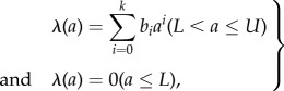
To directly estimate FOI, we used the Grenfell & Anderson [68] model that requires data on human prevalence by age class. This model is derived from the simple catalytic model of Muench [69], which originally assumed that the FOI λ(a) (defined per susceptible individual per unit time) is constant and independent of age a; Grenfell & Anderson [68] generalized this model to a polynomial function (of degree k) of the form

2.1

where U is the upper age limit of human life expectancy (i.e. the oldest age class for which data are available), the lower age threshold L accounts for maternally derived antibodies in children born from mothers who have experienced infection and the b_is are parameters to be estimated; λ(a) is set to zero below L. This model was used to assess whether the FOI estimated from field prevalence data demonstrates a direct relationship with suitability.

We obtained relevant prevalence data from the database of the Ministry of Health of Venezuela, whereas for Argentina we examined appropriate publications and reports (as described in §2b,e). Inclusion criteria for selection were based on, wherever possible: (i) a minimum of six individuals per age class for the calculation of age-class-specific prevalence, (ii) rejecting data with two or more successive age classes with 0% prevalence (particularly in the older age classes), (iii) pooling different years of the same locality (where available), (iv) deleting all houses with any record of recent spraying with insecticide and (v) an available association with a system of geographical coordinates. This data selection process aimed to provide a more homogeneous prevalence dataset (available at http://figshare.com/articles/T_infestans_and_R_prolixus_data/1024617). Once λ(a) was estimated, and as each λ(a) was associated with a given geographical coordinate, we looked for a relationship between suitability and FOI. In most cases, because the data were extremely variable (e.g. from different periods and various social, environmental and control activity situations), we first divided suitability values into equal length classes (between zero and one) and calculated the mean FOI for each class. Preliminary analyses showed a tendency for FOI to flatten out at high suitability values, so we fitted a more flexible sigmoidal-shaped curve, namely the generalized logistic model of the form

2.2

where y is the dependent variable (FOI here), x the independent variable (climatic niche here), A the lower asymptote, C the upper asymptote, M the point of maximum rate of change, B the rate of change and T the point near which asymptotic maximum rate of change occurs. Because we expect FOI = 0 for zero suitability, we a priori set A = 0 and used the Solver tool within Microsoft Excel (with the GRG nonlinear solving algorithm) to calculate the sum of squares (SSQs) as the goodness-of-fit criterion.

(ii). The two-step method

Step 1. Relationship between suitability and vector density

We proceeded in two phases: (i) relating climatic suitability and entomological household infestation, and (ii) relating household infestation to vector density per house. For the former relationship, we could not find any previous analyses relating these two variables, either for Chagas disease vectors or any other disease vectors. As climatic suitability reflects the potential niche of a vector species, we decided to use climatic suitability as a surrogate for the proportion of infested houses.

The second relationship (house infestation to vector density) is motivated on the basis that population size and the extent of regional occupancy by a species are correlated such that a positive occupancy–abundance relationship generally exists [70]. Additionally, it has been established that total population size typically rises faster than occupancy, so that more widely distributed species have higher local densities at sites where they occur than those more restricted in their distribution [71–75]. This pattern has been documented in a large and rapidly growing number of empirical ecological studies [70], providing patterns with a high level of generality, and several mechanisms have been proposed to explain this relationship [76,77].

For Venezuela, we also checked whether other factors (such as house construction material and domestic animal presence) affected the density of bugs per house. In addition, we scaled the bug household density estimated from the infestation per house values in the database of the Ministry of Health of Venezuela; because the number of bugs collected was the result of one man-hour effort, we converted these numbers into actual bug densities per house. It was shown in Rabinovich et al. [78] that for R. prolixus (and in similar rural houses to those referred to in the database used here), this proportion was, on average (pooling different instars and places within a house), approximately 10 : 1 (actual density per house: collected bugs per house with one man-hour effort), and we therefore adjusted accordingly.

Step 2. Relationship between vector density and transmission risk of Trypanosoma cruzi. To convert from bug density per house to FOI, we adopted the model of Tr. cruzi transmission in Rabinovich et al. [79], a binomial transmission model in which neither the vector nor host population dynamics are explicitly considered. Model output is captured by the transmission risk R (the daily probability of seropositive conversion of a susceptible individual per unit time; equivalent to the FOI) as a function of the daily probability P that a susceptible individual suffers an infection if bitten by an infected bug, as

2.3

where n is the number of daily bites by an infected bug on a susceptible individual (and we consider the household as the unit of transmission). Here, n depends on several factors: (i) the average number of bugs per house V, (ii) the average proportion of bugs that are infected I, (iii) the number of bites an average bug makes per day f, (iv) the average proportion of bites that are made on humans F and (v) the average number of susceptible people in the household H. We used the estimate of P for T. infestans in Argentina from Rabinovich et al. [79] as 0.00198 (95% CI: 0.00029–0.00367) and because there are currently no estimates of P for R. prolixus, we assumed close similarity between the species and adopted a rounded value of P = 0.002. The value of n was calculated using the formula proposed by Rabinovich et al. [79]:

2.4

Although, in reality, factors influencing n are likely to vary spatially and temporally, we assume for this analysis (for projections over many decades) that these values remain approximately constant (except for V, which is calculated in Step 1 as a function of suitability); we assume standard literature values for Venezuela and Argentina as I = 0.2, F = 0.5, f = 0.143 (equivalent to bugs feeding once every 7 days), and H = 4.6 (which is multiplied by 0.9, the average proportion of susceptible individuals per household). Because the contact rate was defined per day, n was multiplied by 365 to convert R to an annual value. We calculated the FOI for states/provinces at high-to-moderate risk of vectorial Chagas disease transmission in Venezuela and Argentina. To estimate the expected number of new cases in 2050, we first linearly projected the current rural population (considered to be the more vulnerable population owing to the higher relative vector exposure compared with urban populations) by a demographic factor of 0.61 in Argentina [80] and 0.74 [80] in Venezuela. We then estimated the average FOI for those states/provinces at high Tr. cruzi transmission risk using QGIS Desktop (v. 2.0.1) [66]. Finally, we estimated the total number of new cases of Tr. cruzi as the product of the rural population size for each state/province and the corresponding average localized FOI, repeating for both the current and 2050 conditions. We also estimated the ‘relative contribution’ (%) of each state/province to the overall predicted incidence, as the ratio of the predicted number of new cases per state/province and the total number of new cases across all states/provinces at high Tr. cruzi transmission risk, for current and 2050 conditions.

3. Results

(a). Changes in climatic suitability for Rhodnius prolixus and Triatoma infestans, from current to 2050 conditions

PCA indicated that 15 of 19 bioclimatic variables on the first two principal components account for 68.8% and 73.8% of the explained variance for R. prolixus and T. infestans, respectively. For both species, the ENMs were based on the following 15 variables: bio01, bio03, bio05, bio06, bio08, bio09, bio10, bio11, bio12, bio13, bio14, bio16, bio17, bio18, bio19 (see §1 in the electronic supplementary material). For both species, comparison of suitability changes between the RCP4.5, RCP6.0 and RCP8.5 scenarios revealed no significant differences using a non-parametric test (see §2 in the electronic supplementary material; table S1 shows suitability statistics per scenario and per species, and electronic supplementary material, table S2 shows confidence intervals of the suitability differences between pairs of scenarios). Therefore, we restricted our analysis only to the intermediate scenario (RCP6.0), which considerably reduced the amount of data handling, processing and storage. Despite full analysis being restricted to scenario RCP6.0, tables S3 and S4 in §3 of the electronic supplementary material summarize the relative frequency of each class of suitability transitions from current to 2050 for T. infestans and R. prolixus, under the three climatic scenarios.

The average MaxEnt model fitted for current climate conditions showed a pAUC ratio of 1.001 and 1.055 for R. prolixus and T. infestans, respectively (table 1). The accuracy of the model's predictions tested by the independent dataset showed that for R. prolixus, 84.2% of coordinates with confirmed presence were predicted as ‘presence points' (i.e. suitability values were higher than the 10th percentile training presence logistic threshold), whereas for T. infestans, 93.5% of the coordinates with confirmed presence were predicted as ‘presence points' (electronic supplementary material, see §4).

Table 1.

Summary of statistics describing the pAUC ratios from omission threshold of 5% and 1000 bootstrap replicates, for R. prolixus and T. infestans.

	R. prolixus	T. infestans
minimum	0.9674	1.0292
maximum	1.0169	1.0923
mean	1.0014	1.0551
standard deviation	0.0132	0.009

The most important bioclimatic factors for both species (after application of the Jackknife procedure) were mainly related to temperature and, to a lesser extent, precipitation. For R. prolixus, the most important variable was the minimum temperature of the coldest month, followed by isothermality, mean temperature of the driest quarter, mean temperature of the coldest quarter, precipitation of the wettest month, precipitation of the wettest quarter and annual precipitation. For T. infestans, the most important predictor variable was the mean temperature of the coldest quarter, followed by isothermality, and the minimum temperature of the coldest month.

For Venezuela, estimates of suitability ranged from 0.029 to 0.75 (mean 0.50, standard deviation (s.d.) 0.099, coefficient of variation (COV) 19% and N = 10 745) for the current conditions, and between 0.023 and 0.83 (mean 0.59, s.d. 0.16, COV 26%, and N = 10 745) for 2050. For Argentina, suitability ranged from 0.0047 to 0.67 (mean 0.49, s.d. 0.14, COV 29%, N = 24 957) for the current conditions, and between 0.0058 and 0.84 (mean 0.41, s.d. 0.16 COV 30%, N = 24 957) for 2050.

Both species show unchanged medium suitability transition class as the dominant one between current and 2050 conditions (figure 1). The relative frequency of this transition class was 46% for R. prolixus and 71% for T. infestans.

Figure 1.

Climatic suitability changes from current to 2050 conditions for (a) R. prolixus and (b) T. infestans. Colours indicate climatic suitability transitions between the three main suitability categories (low, medium and high). (Online version in colour.)

For R. prolixus, current states at high-risk transmission (located along the ‘llanos' on the northwest of Venezuela) show a 6% decrease from medium-to-low suitability in future climatic conditions (figure 1a), whereas current states at low risk (i.e. Amazonas, Bolivar and Apure located in the centre and southeast of Venezuela) show a 40% increase from medium-to-high suitability under future climatic changes. For T. infestans, a considerable area of the provinces at high-to-moderate risk (located across the Chaco biogeographic province) show a 20% decrease from medium-to-low future climatic suitability (figure 1b). This suitability decrease includes northeastern (Formosa, Chaco, Santiago del Estero) and western areas (Catamarca, La Rioja and San Juan) of Argentina. Additionally, both species show unchanged low suitability areas along the Andes mountain range in South America, where the northeastern extreme corresponds to Venezuela and the southeastern extreme to Argentina.

(b). Impact of climate change on the vectorial transmission of Chagas disease

Conversion from suitability to FOI worked considerably better with the one-step method in Argentina and the two-step method in Venezuela.

(i). The one-step method applied to Argentina

We retrieved 56 localities from five countries (28 from Argentina, two from Bolivia, three from Brazil, 21 from Chile and two from Paraguay). However, many were not subsequently included in our analysis, either because the data were pooled for large areas, too few age classes were recorded, or the data were subjected to strong vector control interventions. Applying our inclusion criteria left 15 localities, and once these 15 coordinates with suitability and FOI values had been extracted, the results showed a significant fit to the generalized logistic model (equation (2.2)). The best-fit parameter values (and t-test statistics) were B = 38.653 (1.03 × 10⁻⁶), C = 12.092 (1.24 × 10⁻⁷), M = 0.979 (2.33 × 10⁻⁶) and T = 1.978 (1.033 × 10⁻⁶); figure 2 shows the expected FOI values with their 95% confidence intervals.

Figure 2.

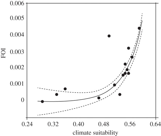
Fit of FOI as a function of climatic suitability of T. infestans.

For T. infestans, the current climatic conditions indicate medium suitability values along the majority of provinces at high-to-moderate transmission risk (figure 3), excluding the western side of the country which instead demonstrated low suitability values. The 4751 new cases of Tr. cruzi human infection per year predicted for all provinces at high-to-moderate transmission risk (black bar, figure 3) under current conditions are considerably greater than the 1581 cases predicted for the same provinces in 2050 (blue/grey bar, figure 3). Currently, four provinces (Córdoba, Santiago del Estero, Tucumán and Mendoza) captured more than 56% of the relative contribution to the total number of predicted new cases. The most significant decrease in incidence is observed in three provinces in the northeast of Argentina: Formosa, Chaco and Santiago del Estero. These provinces, currently at high risk, show not only a decrease in the predicted number of new cases in 2050, but also a decrease from medium-to-low climatic suitability. The pie charts (figure 3) provide us with an overall picture of the degree of change from the present to 2050 in terms of the ‘relative contribution’ (%) of each province at high risk to the total number of predicted new cases. The mean FOI and total number of new cases for each province are summarized in tables S5 and S6 in §5 of the electronic supplementary material.

Figure 3.

Current climatic suitability (base map green to red/grey to black colours) and predicted number of new human cases of Tr. cruzi infection (current: black bar, 2050: blue/grey bar) in Argentina. Provinces were numerated (white circle on the map) to facilitate the identification on the pie charts (number preceding name). Pie charts indicate the ‘relative contribution’ (%) of each province to the total number of new predicted cases over all high transmission risk provinces. Upper pie chart: current conditions; lower pie chart: 2050 conditions. (Online version in colour.)

(ii). The two-step method applied to Venezuela

The density of bugs per house in the 73 selected localities from the database of the Ministry of Public Health of Venezuela was fitted significantly to suitability using the Gaston & He model [81]. However, the predicted densities showed an exponential increase at high climatic suitability values, a pattern different from our observed data, which showed a flattening out of vector density for high values of climatic suitability. To reduce the heterogeneity in the observed density of bugs per house, we estimated its average according to six equal-sized classes of climatic suitability. Because the flattening out of vector density for high house infestation values was still evident, we again fitted the generalized logistic function (equation (2.2)) in order to capture the sigmoidal shape of this relationship. The parameters of the logistic model (equation (2.2)) were C = 0.371, M = 0.401, B = 294.13 and T = 21.22. (SSQ = 0.0014, with one-degree of freedom, and p = 0.030; figure 4).

Figure 4.

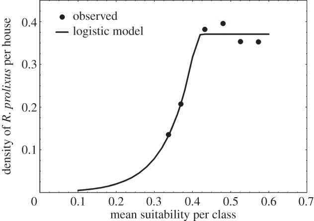
Density of R. prolixus bugs per explored house and mean current climatic suitability per class. Vector densities are in the original one man-hour collection units averaged for each suitability class and not corrected by the ‘catchability’ factor.

The generalized logistic function predicts an asymptotic vector density of about 30 bugs per explored house after applying the ‘catchability’ correction factor. While this appears to be a fairly low density, it is expressed as bugs per explored house and the density distribution is extremely clumped (80% or more of the houses do not harbour any vectors), so this average implies a small, but significant, proportion of houses with several hundred insects. We tried to further improve our predictions of vector densities by additionally accounting for the number of animals in the house and the house construction material, but despite frequent reporting that triatomine densities are related to these factors, we were unable to significantly improve the generalized logistic model fit. Once the vector density (per explored house) was estimated, this was used within the binomial transmission model (equations (2.3) and (2.4)) using average parameter values from the Venezuelan database (I = 0.2, f = 0.5, F = 0.143, H = 4.6, and an assumed proportion of susceptible people within a household of 0.9). The results of these combined steps are shown in figure 5.

Figure 5.

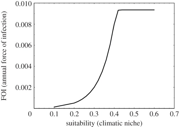
Results of the two-step procedure to estimate FOI from climatic suitability for R. prolixus in Venezuela.

Table S7 in §5 of the electronic supplementary material gives the mean FOI values estimated by the two-step method for each high transmission risk state in Venezuela; these are compared with those estimated by the one-step method in figure 6. In general, and in agreement with the climatic suitability values and figure 1a, there is an overall tendency towards a decrease in incidence in most states at high risk of vectorial transmission in Venezuela from present to 2050 conditions (figure 7). The current annual total of 4677 new human cases of Tr. cruzi infection predicted for all states at high risk of vectorial transmission (black bar, figure 7) is greater than the 3690 predicted new cases in 2050 (blue/grey bar, figure 7). All states, at high risk, contribute a similar relative percentage to both current and future new cases. The most significant decrease in incidence from current to 2050 is observed in Cojedes (from 303 to 116 new cases), whereas the most significant increase (and indeed the only state demonstrating an increase at all) is in Falcón (from 317 to 374 new cases); for more details, see table S8 in §5 of the electronic supplementary material.

Figure 6.

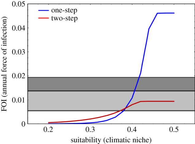
FOI predicted values by both the one-step (blue/black line) and two-step (red/grey line) methods for R. prolixus in Venezuela. Horizontal bands are FOI estimates used as reference values (white lower band = 0–0.005; light grey band = 0.005–0.015; dark grey band = 0.015–0.019). (Online version in colour.)

Figure 7.

Current climatic suitability (base map green to red/grey to black colours) and predicted number of new cases of Tr. cruzi human infection (current: black bar, 2050: blue/grey bar) in Venezuela. States were numerated (white circle on the map) to facilitate the identification on the pie charts (number preceding name). Pie charts indicate the ‘relative contribution’ (%) of each province to the total number of new predicted cases over all high transmission risk states. Upper pie chart, current conditions; lower pie chart, 2050 conditions. (Online version in colour.)

4. Discussion

All temperature-related variables were important in determining the climatic suitability of both species, with a dominant contribution from the minimum temperatures of coldest months. However, for R. prolixus, precipitation variables were also related to climatic suitability. This is consistent with the biology [25] and ecology of this species [82], which inhabits predominantly tropical savannahs and foothills (500–1500 m.a.s.l.) with climatic conditions typically consisting of highly variable rains and temperatures. For T. infestans, the same thermal variables, except the minimum temperature of the driest quarter, were also the most important factors determining the climatic suitability; this is also consistent with the biology of this temperate species that is well adapted to areas characterized by cold temperatures and a broad thermal-tolerance range [83].

The wide areas in Venezuela (mostly in central and southeastern regions) where R. prolixus shows transitions from medium to high suitability suggest a potential shift in its geographical distribution. Because these areas are currently considered at low transmission risk, new vectorial transmission seems a distinct possibility for Venezuela in the climatic change scenario considered here (RCP6.0). On the other hand, the predicted decrease from medium-to-low suitability in high-risk Tr. cruzi transmission states in Venezuela suggests a decrease in the geographical distribution of this species, mainly at the foothills of the Andean and coastal mountain ranges, thus suggesting less serious epidemiological implications in a climate change context. In contrast, no changes from medium-to-high climatic suitability were observed for T. infestans in Argentina, but instead a marked change from medium-to-low suitability (mainly in northeast and western provinces of Argentina) may occur, thus suggesting a decrease in the geographical distribution of this species. This result agrees with both empirical field data and ecogeographical models [84], which suggest that T. infestans has a limited ability to thrive in a warm and humid climate.

Many studies to date addressing the question of climate change impacts on vector-borne diseases have suggested that environmental change is likely to strengthen transmission potential and expand the geographical range of disease vectors into, for example, higher latitudes [85]. However, recent studies suggest a shift (rather than expansion) in the geographical distribution of species and vector-borne diseases in a global warming context [85–87], which is consistent with our results for both R. prolixus and T. infestans as well as other triatomine studies [37,38]. In accounting for the fact that insects adapted to higher latitudes may present a broader thermal-tolerance range than those adapted to lower latitudes, some authors have proposed that tropical organisms will be more sensitive to temperature changes [88] and consequently, the impact of climate change will be different across latitudes and species [89]. In agreement with these considerations, we observed a differential impact of climate change on the two vector species analysed here: R. prolixus shows a future expansion to new areas, whereas T. infestans shows a future decrease in its geographical range compared with current conditions.

Several authors, based on sample theory models, have proposed a link between presence (or occupancy) of species and their population abundance [70,72,81,90]. Despite the fact that the house infestation–vector density relationship used here is beginning to become recognized in certain other vector species such as phlebotomine sandflies associated with the transmission of leishmaniasis [85], R. prolixus and T. infestans do not seem to show such a direct relationship, and this could be due to the existence of other variables (socio-environmental or economic among others) that were not included in our ecological niche models. Because the climatic suitability estimated by the ENMs does not take into account socio-environmental variables such as vector control strategies, the relationship between occupancy and population abundance becomes difficult to verify. Socio-environmental variables, as well as many other factors such as the adequate criterion of spatial and temporal scale selection, remain to be addressed for full application of ENMs to disease systems [29], and this may affect the precision and accuracy of predictions about the likely future behaviour of disease transmission under climate change [91]. Similarly, Roura-Pascual et al. [92] claim that proper choice of environmental datasets is important, because climatic data provide longer temporal applicability. Although remotely sensed data can provide finer spatial resolution, by measuring aspects of ecologic landscapes that climate parameters alone may not capture, we used variables provided by weather stations (interpolated data) because these represent the only available datasets for future conditions. Additionally, comparison between predictions for current and future conditions could be problematic, because the current bioclimatic variables could be far from reality (observed climatic data).

Our use of climatic variables to predict species suitability as a surrogate for population densities has been the subject of few ecological studies to study the epidemiology of vector-borne diseases. Given that the entomological database was reduced to decrease the high heterogeneity observed, we note that our results should be cautiously interpreted in the context of the large uncertainties present in epidemiological and climatic data, and thus unavoidably inherent in the integrated modelling approach developed here. Potential changes in the transmission risk of Tr. cruzi should also not be used as indicators of short-term vectorial control decisions, but rather cautiously interpreted as indicators of a potential longer-term trend given the best available current entomological and epidemiological data.

Despite these heterogeneous results, our main conclusions point to a decreasing trend in the number of new human cases of Tr. cruzi infection per year between current and future conditions. However, it is important to be aware of recent (and ongoing) decreases in the size of the rural population; future demographic projections for rural populations in 2050 predict a decrease in size of 26% and 49% for Venezuela and Argentina [80], respectively. This implies that even if an FOI value remains constant between current and future scenarios, a decrease in incidence suggests a decreasing risk; however, this would lead to a false conclusion in the event of a decrease in the rural population size. For R. prolixus, our FOI estimates were of a similar order of magnitude as those previously estimated for Venezuela by Feliciangeli et al. [42] for the period prior to the initiation of the National Campaign for Chagas Disease Control. Our conversion from FOI to incidence could have been improved further by considering only susceptible individuals from the rural population. Additionally, we could also have separated ‘marginally dispersed’ and plain ‘rural’ populations as undertaken by Chuit [93] in relation to Chagas disease. However, these additional details would have taken us beyond the main purpose of this manuscript and are unlikely to have substantially affected the key qualitative conclusions drawn.

In relation to the use of occurrence points from geographical range maps, it is well known that range maps are not able to capture environmental areas where the species is actually absent within its distribution. Although this is not the usual approach to model species distributions since it may overestimate the geographical distribution of a species introducing a great number of false positives, the presence points derived from geographical distribution atlas allow us to understand large-scale distribution patterns of species [94,95]. Nevertheless, the use of data based upon individual occurrences from surveys would not necessarily produce more accurate suitability predictions, because this kind of data may itself introduce uncertainties related to different sampling efforts, both in space and time, introducing cases of false negatives. Particularly for T. infestans and R. prolixus, even if several occurrence points could be compiled from the literature, these points would not represent the geographical distribution of these species because they do not respond to a specific ecological sampling design and are, generally, biased to certain study areas. In our case, because the main goal was to analyse the effect of climate change on Chagas disease transmission, it was decided that it was preferable to overestimate the potential transmission risk (owing to false positives) than to underestimate it (owing to false negatives).

In addition to the caveats identified above, we have analysed only one of the various possible downscaled prediction models (HadGEM2-ES), and only one of the future projection periods (2050). Limitations arising from the spatial resolution and interpolation process associated with the WorldClim dataset should also be noted, in particular, because there are fewer weather stations in Latin America compared with those in other parts of the world (forcing interpolation between larger distances). Because of the uncertainties associated with the climatic variables, the inference of the Tr. cruzi transmission risk based on climatic suitability of vector species, require the incorporation of other environmental variables and/or socioeconomic factors, which likely affect the estimation of disease incidence. Further research is therefore needed to more thoroughly assess the robustness and generality of our conclusions about future Tr. cruzi transmission risk, which are affected here by the range of uncertainties that unavoidably arise from an integrated modelling approach based on ecological, epidemiological and climatic factors.

Funding statement

This work was supported by the Agencia Nacional de Promoción Científica y Tecnológica of Argentina (grant PICT2008-0035) to J.E.R., and by the Wellcome Trust through a student grant to A.F., and materials and fieldwork expenses (project no. 062984/Z/00Z, leader Clive Davies; 2002–2007).

References

- 1.Intergovernmental Panel on Climate Change. 2007. Climate change 2007: synthesis report. Geneva, Switzerland: IPCC. [Google Scholar]
- 2.Gage KL, Burkot TR, Eisen RJ, Hayes EB. 2008. Climate and vectorborne diseases. Am. J. Prev. Med. 35, 436–450. ( 10.1016/j.amepre.2008.08.030) [DOI] [PubMed] [Google Scholar]
- 3.Mills JN, Gage KL, Khan AS. 2010. Potential influence of climate change on vector-borne and zoonotic diseases: a review and proposed research plan. Environ. Health Perspect. 118, 1507–1514. ( 10.1289/ehp.0901389) [DOI] [PMC free article] [PubMed] [Google Scholar]
- 4.Mills JN. 2005. Regulation of rodent-borne viruses in the natural host: implications for human disease. In Infectious diseases from nature: mechanisms of viral emergence and persistence (eds CJ Peters, CH Calisher), pp. 45–57. Vienna, Austria: Springer. [DOI] [PubMed] [Google Scholar]
- 5.World Health Organization 2013. Sustaining the drive to overcome the global impact of neglected tropical diseases: second WHO report on neglected diseases. Geneva, Switzerland: WHO. [Google Scholar]
- 6.Galvão C, Carcavallo RU, Da Silva Rocha D, Jurberg J. 2003. A checklist of the current valid species of the subfamily Triatominae Jeannel, 1919 (Hemiptera, Reduviidae) and their geographical distribution, with nomenclatural and taxonomic notes. Zootaxa 36, 1–36. [Google Scholar]
- 7.Schofield CJ, Galvão C. 2009. Classification, evolution, and species groups within the Triatominae. Acta Trop. 110, 88–100. ( 10.1016/j.actatropica.2009.01.010) [DOI] [PubMed] [Google Scholar]
- 8.Rabinovich JE, Kitron UD, Obed Y, Yoshioka M, Gottdenker N, Chaves LF. 2011. Ecological patterns of blood-feeding by kissing-bugs (Hemiptera: Reduviidae: Triatominae). Mem. Inst. Oswaldo Cruz 106, 479–94. ( 10.1590/S0074-02762011000400016) [DOI] [PubMed] [Google Scholar]
- 9.Rodrigues Coura J. 2013. Chagas disease: control, elimination and eradication. Is it possible? Mem. Inst. Oswaldo Cruz 108, 962–967. ( 10.1590/0074-0276130565) [DOI] [PMC free article] [PubMed] [Google Scholar]
- 10.Moncayo A. 1992. Chagas disease: epidemiology and prospects for interruption of transmission in the Americas. World Health Stat. Q. 45, 276–279. [PubMed] [Google Scholar]
- 11.Carcavallo R, Galíndez Girón I, Jurberg J, Lent H. 1999. Geographical distribution and alti-latitudinal dispersion of Triatominae. In Atlas of Chagas’ disease vectors in the Americas, vol. 3 (eds Carcavallo RU, Galíndez Girón I, Jurberg J, Lent H.), pp. 747–792. Rio de Janeiro, Brasil: FIOCRUZ. [Google Scholar]
- 12.World Health Organization Expert Committee 2000. Control of Chagas disease second report of the WHO expert committee. Brasilia, Brazil: WHO. [Google Scholar]
- 13.Guhl F. 2009. Enfermedad de Chagas: Realidad y perspectivas. Rev. Biomed. 20, 228–234. [Google Scholar]
- 14.Schofield CJ. 1994. Triatominae: biology & control. West Sussex, UK: Eurocommunica. [Google Scholar]
- 15.Carcavallo RU, Tonn RJ, Carrasquero B. 1977. Distribution of triatominae in Venezuela, (Hemiptera, Reduviidae). Updated by entities and biogeographical zones. Boletín Malariol. y Saneam. Ambient. 17, 53–65. [Google Scholar]
- 16.Lent H, Wygodzinsky P. 1979. Revision of the Triatominae (Hemiptera, Reduviidae), and their significance as vectors of chagas’ disease. Bull. Am. Museum Nat. Hist. 163, 123–520. [Google Scholar]
- 17.Ceballos LA, et al. 2011. Hidden sylvatic foci of the main vector of Chagas disease Triatoma infestans: threats to the vector elimination campaign? PLoS Negl. Trop. Dis. 5, e1365 ( 10.1371/journal.pntd.0001365) [DOI] [PMC free article] [PubMed] [Google Scholar]
- 18.Lazzari CR. 1991. Temperature preference in Triatoma infestans (Hemiptera: Reduviidae). Bull. Entomol. Res. 81, 273–276. ( 10.1017/S0007485300033538) [DOI] [Google Scholar]
- 19.Schilman PE, Lazzari CR. 2004. Temperature preference in Rhodnius prolixus, effects and possible consequences. Acta Trop. 90, 115–122. ( 10.1016/j.actatropica.2003.11.006) [DOI] [PubMed] [Google Scholar]
- 20.Canals M, Solis R, Valderas J, Ehrenfeld M, Cattan PE. 1997. Preliminary studies on temperature selection and activity cycles of Triatoma infestans and T. spinolai (Heteroptera: Reduviidae), Chilean vectors of Chagas’ disease. J. Med. Entomol. 34, 11–17. [DOI] [PubMed] [Google Scholar]
- 21.Clark N. 1935. The effect of temperature and humidity upon the eggs of the bug, Rhodnius prolixus (Heteroptera, Reduviidae). J. Anim. Ecol. 1, 82–87. ( 10.2307/1215) [DOI] [Google Scholar]
- 22.Lazzari CR, Núñez JA. 1989. The response to radiant heat and the estimation of the temperature of distant sources in Triatoma infestans. J. Insect Physiol. 35, 525–529. ( 10.1016/0022-1910(89)90060-7) [DOI] [Google Scholar]
- 23.Ferreira RA, Lazzari CR, Lorenzo MG, Pereira MH. 2007. Do haematophagous bugs assess skin surface temperature to detect blood vessels? PLoS ONE 2, e932 ( 10.1371/journal.pone.0000932) [DOI] [PMC free article] [PubMed] [Google Scholar]
- 24.Fresquet N, Lazzari CR. 2011. Response to heat in Rhodnius prolixus: the role of the thermal background. J. Insect Physiol. 57, 1446–1449. ( 10.1016/j.jinsphys.2011.07.012) [DOI] [PubMed] [Google Scholar]
- 25.Luz C, Fargues J, Grunewald J. 1999. Development of Rhodnius prolixus (Hemiptera: Reduviidae) under constant and cyclic conditions of temperature and humidity. Mem. Inst. Oswaldo Cruz 94, 403–409. ( 10.1590/S0074-02761999000300022) [DOI] [PubMed] [Google Scholar]
- 26.Okasha AYK. 1964. Effects of high temperature in Rhodnius prolixus (Stal). Nature 204, 1221–1222. ( 10.1038/2041221a0) [DOI] [Google Scholar]
- 27.Okasha AYK. 1968. Effects of sub-lethal high temperature on an insect, Rhodnius prolixus (Stal). III. Metabolic changes and their bearing on the cessation and delay of moulting. Exp. Biol. 48, 475–486. [Google Scholar]
- 28.Okasha AYK. 1968. Changes in the respiratory metabolism of Rhodnius prolixus as induced by temperature. J. Insect Physiol. 14, 1621–1634. ( 10.1016/0022-1910(68)90096-6) [DOI] [Google Scholar]
- 29.Peterson AT. 2006. Ecologic niche modeling and spatial patterns of disease transmission. Emerg. Infect. Dis. 12, 1822–1826. ( 10.3201/eid1212.060373) [DOI] [PMC free article] [PubMed] [Google Scholar]
- 30.Peterson AT, Soberón J, Pearson RG, Anderson RP, Martínez-Meyer E, Nakamura M, Araújo MB. 2011. Ecological niches and geographic distributions. Princeton, NJ: Princeton University Press. [Google Scholar]
- 31.Holt RD, Gomulkiewicz R. 1997. The evolution of specieś niches: a population dynamic perspective. In Case studies in mathematical modelling: ecology, physiology, and cell biology (eds Othmer FR, Adler RF, Lewis MA, Dallon JC.), pp. 25–50. Englewood Cliffs, NJ: Prentice Hall. [Google Scholar]
- 32.Franklin J. 2009. Mapping species distributions: spatial inference and prediction. New York, NY: Cambridge University Press. [Google Scholar]
- 33.Peterson AT. 2008. Biogeography of diseases: a framework for analysis. Naturwissenschaften 95, 483–491. ( 10.1007/s00114-008-0352-5) [DOI] [PMC free article] [PubMed] [Google Scholar]
- 34.Anderson RP, et al. 2006. Novel methods improve prediction of specieś distributions from occurrence data. Ecography (Cop.). 29, 129–151. ( 10.1111/j.2006.0906-7590.04596.x) [DOI] [Google Scholar]
- 35.Margules CR, Sarkar S. 2007. Systematic conservation planning. Cambridge, UK: Cambridge University Press. [Google Scholar]
- 36.Sarkar S, et al. 2006. Biodiversity conservation planning tools: present status and challenges for the future. Annu. Rev. Environ. Resour. 31, 123–159. ( 10.1146/annurev.energy.31.042606.085844) [DOI] [Google Scholar]
- 37.Costa J, Dornak LL, Almeida CE, Peterson AT. 2014. Distributional potential of the Triatoma brasiliensis species complex at present and under scenarios of future climate conditions. Parasit. Vectors 7, 238 ( 10.1186/1756-3305-7-238) [DOI] [PMC free article] [PubMed] [Google Scholar]
- 38.Garza M, Feria Arroyo TP, Casillas EA, Sanchez-Cordero V, Rivaldi C-L, Sarkar S. 2014. Projected future distributions of vectors of Trypanosoma cruzi in North America under climate change scenarios. PLoS Negl. Trop. Dis. 8, e2818 ( 10.1371/journal.pntd.0002818) [DOI] [PMC free article] [PubMed] [Google Scholar]
- 39.Gurgel-Gonçalves R, Galvão C, Costa J, Peterson AT. 2012. Geographic distribution of Chagas disease vectors in Brazil based on ecological niche modeling. J. Trop. Med. 2012, 705326 ( 10.1155/2012/705326) [DOI] [PMC free article] [PubMed] [Google Scholar]
- 40.Peterson AT, Sánchez-Cordero V, Beard C, Ramsey JM. 2002. Ecologic niche modeling and potential reservoirs for Chagas disease, Mexico. Emerg. Infect. Dis. 8, 662–667. ( 10.3201/eid0807.010454) [DOI] [PMC free article] [PubMed] [Google Scholar]
- 41.Mendes Pereira J, Silva De Almeida P, Vieira De Sousa A, Moraes De Paula A, Machado RB, Gurgel-Gonçalves R. 2013. Climatic factors influencing triatomine occurrence in Central-West Brazil. Mem. Inst. Oswaldo Cruz 108, 335–341. ( 10.1590/S0074-02762013000300012) [DOI] [PMC free article] [PubMed] [Google Scholar]
- 42.Feliciangeli MD, Campbell-Lendrum D, Martinez C, Gonzalez D, Coleman P, Davies C. 2003. Chagas disease control in Venezuela: lessons for the Andean region and beyond. Trends Parasitol. 19, 44–49. ( 10.1016/S1471-4922(02)00013-2) [DOI] [PubMed] [Google Scholar]
- 43.Añez N, Crisante G, Rojas A. 2004. Update on Chagas disease in Venezuela: a review. Mem. Inst. Oswaldo Cruz 99, 781–787. ( 10.1590/S0074-02762004000800001) [DOI] [PubMed] [Google Scholar]
- 44.Schofield CJ, Jannin J, Salvatella R. 2006. The future of Chagas disease control. Trends Parasitol. 22, 583–588. ( 10.1016/j.pt.2006.09.011) [DOI] [PubMed] [Google Scholar]
- 45.Abad-Franch F, Diotaiuti L, Gurgel-Gonçalves R, Gürtler RE. 2013. Certifying the interruption of Chagas disease transmission by native vectors: cui bono? Mem. Inst. Oswaldo Cruz 108, 251–254. ( 10.1590/0074-0276108022013022) [DOI] [PMC free article] [PubMed] [Google Scholar]
- 46.González C, Wang O, Strutz SE, González-Salazar C, Sánchez-Cordero V, Sarkar S. 2010. Climate change and risk of leishmaniasis in North America: predictions from ecological niche models of vector and reservoir species. PLoS Negl. Trop. Dis. 4, e585 ( 10.1371/journal.pntd.0000585) [DOI] [PMC free article] [PubMed] [Google Scholar]
- 47.Malik SM, Awan H, Khan N. 2012. Mapping vulnerability to climate change and its repercussions on human health in Pakistan. Glob. Health 8, 31 ( 10.1186/1744-8603-8-31) [DOI] [PMC free article] [PubMed] [Google Scholar]
- 48.Lambert RC, Kolivras KN, Resler LM, Brewster CC, Paulson SL. 2008. The potential for emergence of Chagas disease in the United States. Geospat. Health 2, 227–239. ( 10.4081/gh.2008.246) [DOI] [PubMed] [Google Scholar]
- 49.Huber O. 1988. Mapa de vegetación de Venezuela. República de Venezuela, Ministerio del Ambiente y de los Recursos Naturales Renovables, Dirección General de Información e Investigación del Ambiente, Dirección de Suelos, Vegetación y Fauna, División de Vegetación.
- 50.Ministry of Public Health of Argentina 2014. El Chagas en el país y América Latina. See http://www.msal.gov.ar/chagas/index.php/informacion-para-ciudadanos/el-chagas-en-el-pais-y-america-latina.
- 51.Cabrera AL, Willink A. 1973. Biogeografia de América Latina. Washington, DC: Organización de los Estados Americanos (OEA). [Google Scholar]
- 52.Sexton JP, McIntyre PJ, Angert AL, Rice KJ. 2009. Evolution and ecology of species range limits. Annu. Rev. Ecol. Evol. Syst. 40, 415–436. ( 10.1146/annurev.ecolsys.110308.120317) [DOI] [Google Scholar]
- 53.Figuera A, Feliciangeli MD, Gorla D, Davies C, Campbell-Lendrum D. 2006. Análisis espacio-temporal y uso de sensores remotos para describir la distribución de la infestación de casas por Rhodnius prolixus en Venezuela (1990–2000). In Proc. the Int. Workshop-Course ‘The use of geographic information systems and remote sensors in public health’ (eds Guhl F, Davies C.), p. 224 Bogotá, Colombia: Memorias del Curso-Taller Internacional ‘El uso de Sistemas de Información Geográfica y Sensores Remotos (SR) en Salud Pública’. [Google Scholar]
- 54.Hijmans RJ, Cameron SE, Parra JL, Jones PG, Jarvis A. 2005. Very high resolution interpolated climate surfaces for global land areas. Int. J. Climatol. 25, 1965–1978. ( 10.1002/joc.1276) [DOI] [Google Scholar]
- 55.Intergovernmental Panel on Climate Change 2014. Climate change 2013: The physical science basis Working Group I contribution to the fifth assessment report of the Intergovernmental Panel on Climate Change Cambridge, UK: Cambridge University Press. [Google Scholar]
- 56.Bellouin N, et al. 2011. The HadGEM2 family of Met Office Unified Model Climate configurations. Geosci. Model. Dev. Discuss. 4, 765–841. ( 10.5194/gmdd-4-765-2011) [DOI] [Google Scholar]
- 57.de la Vega GJ, Medone P, Ceccarelli S, Rabinovich J, Schilman PE. In press. Geographical distribution, climatic variability and thermo-tolerance of Chagas disease vectors. Ecography 38 ( 10.1111/ecog.01028) [DOI] [Google Scholar]
- 58.Abdi H, Williams LJ. 2010. Principal component analysis. Wiley Interdiscip. Rev. Comput. Stat. 2, 433–459. ( 10.1002/wics.101) [DOI] [Google Scholar]
- 59.Statpoint Technologies Inc. 2010. Statgraphics Centurion XVI See http://www.statgraphics.com/version16.htm.
- 60.Phillips SJ, Anderson RP, Schapire RE. 2006. Maximum entropy modeling of species geographic distributions. Ecol. Modell. 190, 231–259. ( 10.1016/j.ecolmodel.2005.03.026) [DOI] [Google Scholar]
- 61.Phillips SJ, Dudík M. 2008. Modeling of species distributions with Maxent: new extensions and a comprehensive evaluation. Ecography (Cop.). 31, 161–175. ( 10.1111/j.0906-7590.2008.5203.x) [DOI] [Google Scholar]
- 62.Phillips SJ, Dudík M, Schapire RE. 2004. A maximum entropy approach to species distribution modeling. In Proc. 21 Int. Conf. on Machine learning, p. 83 New York, NY: Association for Computer Machinery. [Google Scholar]
- 63.Peterson AT, Papeş M, Soberón J. 2008. Rethinking receiver operating characteristic analysis applications in ecological niche modeling. Ecol. Modell. 213, 63–72. ( 10.1016/j.ecolmodel.2007.11.008) [DOI] [Google Scholar]
- 64.Lobo JM, Jiménez-Valverde A, Real R. 2008. AUC: a misleading measure of the performance of predictive distribution models. Glob. Ecol. Biogeogr. 17, 145–151. ( 10.1111/j.1466-8238.2007.00358.x) [DOI] [Google Scholar]
- 65.Barve N. 2008. Tool for partial-ROC. Lawrence, KS: Biodiversity Institute. [Google Scholar]
- 66.QGIS Development Team 2013. QGIS geographic information system. See http://www.qgis.org. [Google Scholar]
- 67.Ryan SJ, McNally A, Johnson LR, Mordecai E, Ben-Horin T, Paaijmans K, Lafferty KD. 2014. Rising suitability and declining severity of malaria transmission in Africa under climate change (http://arxiv.org/abs/1407.7612)
- 68.Grenfell BT, Anderson RM. 1985. The estimation of age-related rates of infection from case notifications and serological data. J. Hyg. (Lond). 95, 419–436. ( 10.1017/S0022172400062859) [DOI] [PMC free article] [PubMed] [Google Scholar]
- 69.Muench H. 1959. Catalytic models in epidemiology. Cambridge, MA: Harvard University Press. [Google Scholar]
- 70.Holt AR, Gaston KJ, He F. 2002. Occupancy–abundance relationships and spatial distribution: a review. Basic Appl. Ecol. 3, 1–13. ( 10.1078/1439-1791-00083) [DOI] [Google Scholar]
- 71.Hanski I. 1982. On patterns of temporal and spatial variation in animal populations. Ann. Zool. Fennici 19, 21–37. [Google Scholar]
- 72.Gaston KJ, Lawton JH. 1990. Effects of scale and habitat on the relationship between regional distribution and local abundance. Oikos 58, 329–335. ( 10.2307/3545224) [DOI] [Google Scholar]
- 73.Hanski I, Kouki J, Halkka A. 1993. Three explanations of the positive relationship between distribution and abundance of species. In Species diversity in ecological communities: historical and geographical perspectives (eds Ricklefs R, Shluter D.), pp. 108–116. Chicago, IL: University of Chicago Press. [Google Scholar]
- 74.Gaston KJ. 1996. The multiple forms of the interspecific abundance–distribution relationship. Oikos 76, 211–220. ( 10.2307/3546192) [DOI] [Google Scholar]
- 75.Gaston KJ. 1994. Rarity. London, UK: Chapman and Hall. [Google Scholar]
- 76.Gaston KJ, Blackburn TM, Lawton JH. 1997. Interspecific abundance-range size relationships: an appraisal of mechanisms. J. Anim. Ecol. 66, 579–601. ( 10.2307/5951) [DOI] [Google Scholar]
- 77.Gaston KJ, Blackburn TM, Greenwood JJD, Gregory RDJ, Quinn RM, Lawton JH. 2000. Abundance–occupancy relationships. J. Appl. Ecol. 37, 39–59. ( 10.1046/j.1365-2664.2000.00485.x) [DOI] [Google Scholar]
- 78.Rabinovich JE, Gürtler RE, Leal JA, Feliciangeli D. 1995. Density estimates of the domestic vector of Chagas disease, Rhodnius prolixus Stål (Hemiptera: Reduviidae), in rural houses in Venezuela. Bull. World Health Organ. 73, 347. [PMC free article] [PubMed] [Google Scholar]
- 79.Rabinovich JE, Wisnivesky-Colli C, Solarz ND, Gürtler RE. 1990. Probability of transmission of Chagas disease by Triatoma infestans (Hemiptera: Reduviidae) in an endemic area of Santiago del Estero, Argentina. Bull. World Health Organ. 68, 737–746. [PMC free article] [PubMed] [Google Scholar]
- 80.Population Division of ECLAC 2013 Long term population estimates and projections 1950–2100 . 2013. Revision. Economic Commission for Latin America and Caribe (ECLAC) See http://www.eclac.cl/celade/proyecciones/basedatos_BD.htm.
- 81.Gaston KJ, He F. 2011. Species occurrence and occupancy. In Biological diversity: frontiers in measurement and assessment (eds Magurran AE, McGill BJ.), pp. 141–151. Oxford, UK: Oxford University Press. [Google Scholar]
- 82.Feliciangeli de Piñero D, Torrealba JW. 1977. Observaciones sobre Rhodnius prolixus (Hemiptera: Reduviidae) en su biotopo silvestre Copernicia tectorum. Boletín la Dir. Malariol. y Saneam. Ambient. 3, 198–205. [Google Scholar]
- 83.Dias E. 1955. Variações mensais da incidência das formas evolutivas do Triatoma infestans e do Panstrongylus megistus no município de Bambuí, Estado de Minas Gerais. Mem. Inst. Oswaldo Cruz 53, 457–472. ( 10.1590/S0074-02761955000200022) [DOI] [PubMed] [Google Scholar]
- 84.Gorla DE. 2002. Variables ambientales registradas por sensores remotos como indicadores de la distribución geográfica de Triatoma infestans (Heteroptera: Reduviidae). Ecol. Austral 12, 117–127. [Google Scholar]
- 85.Lafferty KD. 2009. The ecology of climate change and infectious diseases. Ecology 90, 888–900. ( 10.1890/08-0079.1) [DOI] [PubMed] [Google Scholar]
- 86.Rolandi C, Schilman PE. 2012. Linking global warming, metabolic rate of hematophagous vectors, and the transmission of infectious diseases. Front. Physiol. 3, 75 ( 10.3389/fphys.2012.00075) [DOI] [PMC free article] [PubMed] [Google Scholar]
- 87.Sutherst RW, Maywald G. 2005. A climate model of the red imported fire ant, Solenopsis invicta Buren (Hymenoptera: Formicidae): implications for invasion of new regions, particularly Oceania. Environ. Entomol. 34, 317–335. ( 10.1603/0046-225X-34.2.317) [DOI] [Google Scholar]
- 88.Chown SL, Nicolson S. 2004. Insect physiological ecology: mechanisms and patterns. Oxford, UK: Oxford University Press. [Google Scholar]
- 89.Deutsch CA, Tewksbury JJ, Huey RB, Sheldon KS, Ghalambor CK, Haak DC, Martin PR. 2008. Impacts of climate warming on terrestrial ectotherms across latitude. Proc. Natl Acad. Sci. USA 105, 6668–6672. ( 10.1073/pnas.0709472105) [DOI] [PMC free article] [PubMed] [Google Scholar]
- 90.Martínez-meyer E, Díaz-porras D, Peterson AT, Yáñez-Arenas C. 2012. Ecological niche structure and rangewide abundance patterns of species. Biol. Lett. 9, 169–179. ( 10.1098/rsbl.2012.0637) [DOI] [PMC free article] [PubMed] [Google Scholar]
- 91.Peterson AT, Martínez-Campos C, Nakazawa Y, Martínez-Meyer E. 2005. Time-specific ecological niche modeling predicts spatial dynamics of vector insects and human dengue cases. Trans. R. Soc. Trop. Med. Hyg. 99, 647–655. ( 10.1016/j.trstmh.2005.02.004) [DOI] [PubMed] [Google Scholar]
- 92.Roura-Pascual N, Suarez AV, McNyset K, Gómez C, Pons P, Touyama Y, Wild AL, Gascon F, Peterson AT. 2006. Niche differentiation and fine-scale projections for Argentine ants based on remotely sensed data. Ecol. Appl. 16, 1832–1841. ( 10.1890/1051-0761(2006)016[1832:NDAFPF]2.0.CO;2) [DOI] [PubMed] [Google Scholar]
- 93.Chuit R. 2000. La Enfermedad de Chagas en el Siglo XXI-Argentina. In Fundación Mundo Sano Buenos Aires. Argentina. 1er. Congreso Virtual de Cardiología.
- 94.Diniz-Filho JAF, Bini LM, Rangel TF, Loyola RD, Hof C, Nogués-Bravo D, Araújo MB. 2009. Partitioning and mapping uncertainties in ensembles of forecasts of species turnover under climate change. Ecography (Cop.). 32, 897–906. ( 10.1111/j.1600-0587.2009.06196.x) [DOI] [Google Scholar]
- 95.Lawler JJ, Shafer SL, White D, Kareiva P, Maurer EP, Blaustein AR, Bartlein PJ. 2009. Projected climate-induced faunal change in the Western Hemisphere. Ecology 90, 588–597. ( 10.1890/08-0823.1) [DOI] [PubMed] [Google Scholar]
Associated Data
This section collects any data citations, data availability statements, or supplementary materials included in this article.