Phylogenomics with paralogs

Significance

We demonstrate that the distribution of paralogs in large gene families contains in itself sufficient phylogenetic signal to infer fully resolved species phylogenies. This source of phylogenetic information is independent of information contained in orthologous sequences and is resilient against horizontal gene transfer. An important consequence is that phylogenomics data sets need not be restricted to 1:1 orthologs.

Abstract

Phylogenomics heavily relies on well-curated sequence data sets that comprise, for each gene, exclusively 1:1 orthologos. Paralogs are treated as a dangerous nuisance that has to be detected and removed. We show here that this severe restriction of the data sets is not necessary. Building upon recent advances in mathematical phylogenetics, we demonstrate that gene duplications convey meaningful phylogenetic information and allow the inference of plausible phylogenetic trees, provided orthologs and paralogs can be distinguished with a degree of certainty. Starting from tree-free estimates of orthology, cograph editing can sufficiently reduce the noise to find correct event-annotated gene trees. The information of gene trees can then directly be translated into constraints on the species trees. Although the resolution is very poor for individual gene families, we show that genome-wide data sets are sufficient to generate fully resolved phylogenetic trees, even in the presence of horizontal gene transfer.

Molecular phylogenetics is primarily concerned with the reconstruction of evolutionary relationships between species based on sequence information. To this end, alignments of protein or DNA sequences are used, whose evolutionary history is believed to be congruent to that of the respective species. This property can be ensured most easily in the absence of gene duplications and horizontal gene transfer (HGT). Phylogenetic studies judiciously select families of genes that rarely exhibit duplications (such as rRNAs, most ribosomal proteins, and many of the housekeeping enzymes). In phylogenomics, elaborate automatic pipelines such as HaMStR (1), are used to filter genome-wide data sets to at least deplete sequences with detectable paralogs (homologs in the same species).

In the presence of gene duplications, however, it becomes necessary to distinguish between the evolutionary history of genes (gene trees) and the evolutionary history of the species (species trees) in which these genes reside. Leaves of a gene tree represent genes. Their inner nodes represent two kinds of evolutionary events, namely the duplication of genes within a genome—giving rise to paralogs—and speciations, in which the ancestral gene complement is transmitted to two daughter lineages. Two genes are (co)orthologous if their last common ancestor in the gene tree represents a speciation event, whereas they are paralogous if their last common ancestor is a duplication event; see refs. 2 and 3 for a more recent discussion on orthology and paralogy relationships. Speciation events, in turn, define the inner vertices of a species tree. However, they depend on both the gene and the species phylogeny, as well as the reconciliation between the two. The latter identifies speciation vertices in the gene tree with a particular speciation event in the species tree and places the gene duplication events on the edges of the species tree. Intriguingly, it is nevertheless possible in practice to distinguish orthologs with acceptable accuracy without constructing either gene or species trees (4). Many tools of this type have become available over the last decade; see refs. 5 and 6 for a recent review. The output of such methods is an estimate $\mathrm{\Theta }$ of the true orthology relation ${\mathrm{\Theta }}^{\mathrm{\ast }}$, which can be interpreted as a graph $G_{\mathrm{\Theta }}$ whose vertices are genes and whose edges connect estimated (co)orthologs.

Recent advances in mathematical phylogenetics suggest that the estimated orthology relation $\mathrm{\Theta }$ contains information on the structure of the species tree. To make this connection, we combine here three abstract mathematical results that are made precise in Materials and Methods below.

• i)Building upon the theory of symbolic ultrametrics (7), we showed that in the absence of horizontal gene transfer, the orthology relation of each gene family is a cograph (8). Cographs can be generated from the single-vertex graph $K_1$ by complementation and disjoint union (9). This special structure of cographs imposes very strong constraints that can be used to reduce the noise and inaccuracies of empirical estimates of orthology from pairwise sequence comparison. To this end, the initial estimate of $G_{\mathrm{\Theta }}$ is modified to the closest correct orthology relation $G_{{\mathrm{\Theta }}^{\mathrm{\ast }}}$ in such a way that a minimal number of edges (i.e., orthology assignments) are introduced or removed. This amounts to solving the cograph-editing problem (10, 11).
• ii)It is well known that each cograph is equivalently represented by its cotree (9). The cotree is easily computed for a given cograph. In our context, the cotree of $G_{{\mathrm{\Theta }}^{\mathrm{\ast }}}$ is an incompletely resolved event-labeled gene tree. That is, in addition to the tree topology, we know for each internal branch point whether it corresponds to a speciation or a duplication event. Even though adjacent speciations or adjacent duplications cannot be resolved, the tree faithfully encodes the relative order of any pair of duplication and speciation (8). In the presence of horizontal gene transfer, $G_{\mathrm{\Theta }}$ may deviate from the structural requirements of a cograph. Still, the situation can be described in terms of edge-colored graphs whose subgraphs are cographs (7, 8), so that the cograph structure remains an acceptable approximation.
• iii)Every triple (rooted binary tree on three leaves) in the cotree that has leaves from three species and is rooted in a speciation event also appears in the underlying species tree (12). Thus, the estimated orthology relation, after editing to a cograph and conversion to the equivalent event-labeled gene tree, provides much information on the species tree. This result allows us to collect, from the cotrees for each gene family, partial information on the underlying species tree. Interestingly, only gene families that harbor duplications, and thus have a nontrivial cotree, are informative. If no paralogs exist, then the orthology relation $G_{\mathrm{\Theta }}$ is a clique (i.e., every family member is orthologous to every other family member) and the corresponding cotree is completely unresolved, and hence contains no triple. On the other hand, full resolution of the species tree is guaranteed if at least one duplication event between any two adjacent speciations is observable. The achievable resolution therefore depends on the frequency of gene duplications and the number of gene families.

Despite the variance reduction due to cograph editing, noise in the data, as well as the occasional introduction of contradictory triples as a consequence of horizontal gene transfer, is unavoidable. The species triples collected from the individual gene families thus will not always be congruent. A conceptually elegant way to deal with such potentially conflicting information is provided by the theory of supertrees in the form of the largest set of consistent triples (13, 14). The data will not always contain a sufficient set of duplication events to achieve full resolution. To this end, we consider trees with the property that the contraction of any edge leads to the loss of an input triple. There may be exponentially many alternative trees of this type. They can be listed efficiently using Semple’s algorithms (15). To reduce the solution space further, we search for a least resolved tree in the sense of ref. 16, i.e., a tree that has the minimum number of inner vertices. It constitutes one of the best estimates of the phylogeny without pretending a higher resolution than actually supported by the data. In SI Appendix, we discuss alternative choices.

The mathematical reasoning summarized above, outlined in Materials and Methods, and presented in full detail in SI Appendix, directly translates into a computational workflow, Fig. 1. It entails three NP-hard combinatorial optimization problems: cograph editing (11), maximal consistent triple set (17–19), and least resolved supertree (16). We show here that they are nevertheless tractable in practice by formulating them as Integer Linear Programs (ILP) that can be solved for both artificial benchmark data sets and real-life data sets, comprising genome-scale protein sets for dozens of species, even in the presence of horizontal gene transfer.

Fig. 1.

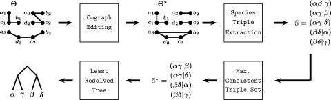
Outline of the computational framework. Starting from an estimated orthology relation $\mathrm{\Theta }$, its graph representation $G_{\mathrm{\Theta }}$ is edited to obtain the closest cograph $G_{{\mathrm{\Theta }}^{\mathrm{*}}}$, which, in turn, is equivalent to a (not necessarily fully resolved) gene tree T and an event labeling t. From $\left(T,t\right)$, we extract the set $\mathbb{S}$ of all relevant species triples. As the triple set $\mathbb{S}$ need not be consistent, we compute the maximal consistent subset ${\mathbb{S}}^{\mathrm{\ast }}$ of $\mathbb{S}$. Finally, we construct a least resolved species tree from ${\mathbb{S}}^{\mathrm{\ast }}$.

Materials and Methods

Preliminaries.

Here, we summarize the definitions and notations required to outline the mathematical framework, presented in Theory and ILP Formulation.

Phylogenetic trees.

We consider a set $\mathfrak{G}$ of at least three genes from a nonempty set $\mathfrak{S}$ of species. We denote genes by lowercase Roman and species by lowercase Greek letters. We assume that for each gene, its species of origin is known. This is encoded by the surjective map $\sigma :\mathfrak{G}\to \mathfrak{S}$ with $a\mapsto \sigma \left(a\right)$. A phylogenetic tree (on L) is a rooted tree $T=\left(V,E\right)$ with leaf set $L\subseteq V$ such that no inner vertex $v\in V^0:=V\backslash L$ has outdegree one and whose root ${\rho }_T\in V$ has indegree zero. A phylogenetic tree T is called “binary” if each inner vertex has outdegree two. A phylogenetic tree on $\mathfrak{G}$, respectively, on $\mathfrak{S}$, is called “gene tree,” respectively, “species tree.” A (inner) vertex y is an ancestor of $x\in V$, in symbols $x{\prec }_{T}y$ if $y\ne x$ lies on the unique path connecting x with ${\rho }_T$. The most recent common ancestor ${\text{lca}}_T\left(L^{\prime }\right)$ of a subset $L^{\prime }\subseteq L$ is the unique vertex in T that is the least upper bound of $L^{\prime }$ under the partial order ${\mathrm{\preccurlyeq }}_T$. We write $L\left(v\right):=\left\{y\in L|y{\mathrm{\preccurlyeq }}_{T}v\right\}$ for the set of leaves in the subtree of T rooted in v. Thus, $L\left({\rho }_T\right)=L$ and $T\left({\rho }_T\right)=T$.

Rooted triples.

Rooted triples (20), i.e., rooted binary trees on three leaves, are a key concept in the theory of supertrees (21, 22). A rooted triple $r=\left(\mathsf{xy}|\mathsf{z}\right)$ with leaf set $L_r=\left\{x,y,z\right\}$ is displayed by a phylogenetic tree T on L if (i) $L_r\subseteq L$ and (ii) the path from x to y does not intersect the path from z to the root ${\rho }_T$. Thus, ${\text{lca}}_T\left(x,y\right){\prec }_T{\text{lca}}_T\left(x,y,z\right)$. A set R of triples is (strictly) dense on a given leaf set L if for each set of three distinct leaves there is (exactly) one triple $r\in R$. We denote by $\mathrm{\Re }\left(T\right)$ the set of all triples that are displayed by the phylogenetic tree T. A set R of triples is consistent if there is a phylogenetic tree T on $L_R:={\displaystyle {\cup }_{r\in R}{L}_r}$ such that $R\subseteq \mathrm{\Re }\left(T\right)$, i.e., T displays (all triples of) R. If no such tree exists, R is said to be inconsistent.

Given a triple set R, the polynomial-time algorithm BUILD (23) either constructs a phylogenetic tree T displaying R or recognizes that R is inconsistent. The problem of finding a phylogenetic tree with the smallest possible number of vertices that is consistent with every rooted triple in R, i.e., a “least resolved tree,” is an NP-hard problem (16). If R is inconsistent, the problem of determining a maximum consistent subset of an inconsistent set of triples is NP-hard and also APX-hard; see refs. 24 and 25. Polynomial time approximation algorithms for this problem and further theoretical results are reviewed by ref. 26.

Triple-closure operations and inference rules.

If R is consistent, it is often possible to infer additional consistent triples. Denote by $\langle R\rangle$ the set of all phylogenetic trees on $L_R$ that display R. The closure of a consistent set of triples R is $\text{cl}\left(R\right)={\displaystyle {\cap }_{T\in \langle R\rangle }\mathrm{\Re }\left(T\right)}$; see refs. 17 and 27−30. We say R is “closed” if $R=\text{cl}\left(R\right)$ and write $R\mathrm{⊢}\left(\mathsf{xy}|\mathsf{z}\right)$ if and only if $\left(\mathsf{xy}|\mathsf{z}\right)\in \mathrm{cl}\left(R\right)$. The closure of a given consistent set R can be computed in $O\left({\left|R\right|}^5\right)$ time (27). Extending earlier work of Dekker (31), Bryant and Steel (27) derived conditions under which $R\mathrm{⊢}\left(\mathsf{xy}|\mathsf{z}\right)\Rightarrow R^{\prime }\mathrm{⊢}\left(\mathsf{xy}|\mathsf{z}\right)$ for some $R^{\prime }\subseteq R$. Of particular importance are the following so-called “2-order” inference rules:

$$\left\{\left(\mathrm{ab}|\mathrm{c}\right),\left(\mathrm{ad}|\mathrm{c}\right)\right\}\mathrm{⊢}\left(\mathrm{bd}|\mathrm{c}\right)$$ [i]

$$\left\{\left(\mathrm{ab}|\mathrm{c}\right),\left(\mathrm{ad}|\mathrm{b}\right)\right\}\mathrm{⊢}\left(\mathrm{bd}|\mathrm{c}\right),\left(\mathrm{ad}|\mathrm{c}\right)$$ [ii]

$$\left\{\left(\mathrm{ab}|\mathrm{c}\right),\left(\mathrm{cd}|\mathrm{b}\right)\right\}\mathrm{⊢}\left(\mathrm{ab}|\mathrm{d}\right),\left(\mathrm{cd}|\mathrm{a}\right).$$ [iii]

Inference rules based on pairs of triples $r_1,r_2\in R$ can imply new triples only if $\left|L_{r_1}\mathrm{\cap }{L}_{r_2}\right|=2$. Hence, in a strictly dense triple set only the three rules above may lead to new triples.

Cograph.

Cographs have a simple characterization as $P_4$-free graphs, that is, no four vertices induce a simple path, although there are a number of equivalent characterizations; see ref. 32. Cographs can be recognized in linear time (33, 34).

Orthology relation.

An empirical orthology relation $\mathrm{\Theta }\subset \mathfrak{G}\times \mathfrak{G}$ is a symmetric, irreflexive relation that contains all pairs $\left(x,y\right)$ of orthologous genes. Here, we assume that $x,y\in \mathfrak{G}$ are paralogs if and only if $x\ne y$ and $\left(x,y\right)\notin \mathrm{\Theta }$. This amounts to ignoring horizontal gene transfer. Orthology detection tools often report some weight or confidence value $w\left(x,y\right)$ for x and y to be orthologs from which $\mathrm{\Theta }$ is estimated using a suitable cutoff. Importantly, $\mathrm{\Theta }$ is symmetric, but not transitive, i.e., it does in general not represent a partition of $\mathfrak{G}$.

Event-labeled gene tree.

Given $\mathrm{\Theta }$, we aim to find a gene tree T with an “event labeling” $t:V^0\to \left\{•,\square \right\}$ at the inner vertices so that, for any two distinct genes $x,y\in L$, $t\left({\text{lca}}_T\left(x,y\right)\right)=•$ if ${\text{lca}}_T\left(x,y\right)$ corresponds to a speciation, and hence $\left(x,y\right)\in \mathrm{\Theta }$ and $t\left({\text{lca}}_T\left(x,y\right)\right)=\square$ if ${\text{lca}}_T\left(x,y\right)$ is a duplication vertex, and hence $\left(x,y\right)\notin \mathrm{\Theta }$. If such a tree T with event-labeling t exists for $\mathrm{\Theta }$, we call the pair $\left(T,t\right)$ a “symbolic representation” of $\mathrm{\Theta }$. We write $\left(T,t;\sigma \right)$ if, in addition, the species assignment map σ is given. A detailed and more general introduction to the theory of symbolic representations is given in SI Appendix.

Reconciliation map.

A phylogenetic tree $S=\left(W,F\right)$ on $\mathfrak{S}$ is a species tree for a gene tree $T=\left(V,E\right)$ on $\mathfrak{G}$ if there is a reconciliation map $\mu :V\to W\mathrm{\cup }F$ that maps genes $a\in \mathfrak{G}$ to species .. such that the ancestor relation ${\mathrm{\preccurlyeq }}_S$ is implied by the ancestor relation ${\mathrm{\preccurlyeq }}_T$. A more formal definition is given in SI Appendix. Inner vertices of T that map to inner vertices of S are speciations, whereas vertices of T that map to edges of S are duplications.

Theory.

In this section, we summarize the main ideas and concepts behind our approach. These are based on our results established in refs. 8 and 12. We consider the following problem: Given an empirical orthology relation $\mathrm{\Theta }$, we want to compute a species tree. To this end, four independent problems as explained below have to be solved.

From estimated orthologs to cographs.

Empirical estimates of the orthology relation $\mathrm{\Theta }$ will in general contain errors in the form of false-positive orthology assignments, as well as false negatives, e.g., due to insufficient sequence similarity. Horizontal gene transfer adds to this noise. Hence an empirical relation Θ will in general not have a symbolic representation. In fact, $\mathrm{\Theta }$ has a symbolic representation $\left(T,t\right)$ if and only if $G_{\mathrm{\Theta }}$ is a cograph (8), from which $\left(T,t\right)$ can be derived in linear time; see also Theorem 5 in SI Appendix. However, the cograph-editing problem, which aims to convert a given graph $G\left(V,E\right)$ into a cograph $G^{\mathrm{\ast }}=\left(V,E^{*}\right)$ with the minimal number $\left|E\hspace{0.17em}△\hspace{0.17em}{E}^{\mathrm{\ast }}\right|$ of inserted or deleted edges, is an NP-hard problem (10, 11). Here, the symbol $△$ denotes the symmetric difference of two sets. In our setting, the problem is considerably simplified by the structure of the input data. The gene set of every living organism consists of hundreds or even thousands of nonhomologous gene families. Thus, the initial estimate of $G_{\mathrm{\Theta }}$ already partitions into a large number of connected components. As shown in Lemma 9 in SI Appendix, it suffices to solve the cograph editing for each connected component separately.

Extraction of all species triples.

From this edited cograph $G_{{\mathrm{\Theta }}^{*}}$, we obtain a unique cotree that, in particular, is congruent to an incompletely resolved event-labeled gene tree $\left(T,t;\sigma \right)$. In ref. 12, we investigated the conditions for the existence of a reconciliation map μ from the gene tree T to the species tree S. Given $\left(T,t;\sigma \right)$, consider the triple set $\mathbb{G}$ consisting of all triples $r=\left(\mathrm{ab}|\mathrm{c}\right)\in \mathrm{\Re }\left(T\right)$ so that (i) all genes $a,b,c$ belong to different species and (ii) the event at the most recent common ancestor of $a,b,c$ is a speciation event, $t\left(\mathrm{lc}{\mathrm{a}}_T\left(a,b,c\right)\right)=•$. From $\mathbb{G}$ and σ, one can construct the following set of species triples:

$$\mathbb{S}=\left\{\left(\alpha \beta |\gamma \right)|\exists \left(\mathrm{ab}|\mathrm{c}\right)\in \mathbb{G}\text{with}\sigma \left(a\right)=\alpha ,\sigma \left(b\right)=\beta ,\sigma \left(c\right)=\gamma \right\}.$$

The main result of ref. 12 establishes that there is a species tree on $\sigma \left(\mathfrak{G}\right)$ for $\left(T,t,\sigma \right)$ if and only if the triple set $\mathbb{S}$ is consistent. In this case, a reconciliation map can be found in polynomial time. No reconciliation map exists if $\mathbb{S}$ is inconsistent.

Maximal consistent triple set.

In practice, we cannot expect that the set $\mathbb{S}$ will be consistent. Therefore, we have to solve an NP-hard problem, namely, computing a maximum consistent subset of triples ${\mathbb{S}}^{\mathrm{\ast }}\subset \mathbb{S}$ (16). The following result (see ref. 14 and SI Appendix) plays a key role for the ILP formulation of triple consistency.

Theorem 1. A strictly dense triple set R on L with $\left|L\right|\ge 3$ is consistent if and only if $\text{cl}\left(R^{\prime }\right)\subseteq R$ holds for all $R^{\prime }\subseteq R$ with $\left|R^{\prime }\right|=2$.

Least resolved species tree.

To compute an estimate for the species tree in practice, we finally compute from ${\mathbb{S}}^{\mathrm{\ast }}$ a least resolved tree S that minimizes the number of inner vertices. Hence, we have to solve another NP-hard problem (24, 25). However, some instances can be solved in polynomial time, which can be checked efficiently by using the next result (see SI Appendix).

Proposition 2. If the tree T inferred from the triple set R by means of BUILD is binary, then the closure $\text{cl}\left(R\right)$ is strictly dense. Moreover, T is unique and hence a least resolved tree for R.

ILP Formulation.

Because we have to solve three intertwined NP-complete optimization problems, we cannot realistically hope for an efficient exact algorithm. We therefore resort to ILP as the method of choice for solving the problem of computing a least resolved species tree S from an empirical estimate of the orthology relation $G_{\mathrm{\Theta }}$. We will use binary variables throughout. Table 1 summarizes the definition of the ILP variables and provides a key to the notation used in this section. In the following, we summarize the ILP formulation. A detailed description and proofs for the correctness and completeness of the constraints can be found in SI Appendix.

Table 1.

The notation used in the ILP formulation

	Definition
Sets and constants
$\mathfrak{G}$	Set of genes
$\mathfrak{S}$	Set of species
${\mathrm{\Theta }}_{ab}$	Genes $a,b\in \mathfrak{G}$ are estimated orthologs: ${\mathrm{\Theta }}_{ab}=1$ iff $\left(a,b\right)\in \mathrm{\Theta }$
Binary variables
$E_{xy}$	Edge set of the cograph $G_{{\mathrm{\Theta }}^{\mathrm{\ast }}}=\left(\mathfrak{G},E_{{\mathrm{\Theta }}^{\mathrm{\ast }}}\right)$ of the closest relation ${\mathrm{\Theta }}^{\mathrm{\ast }}$ to $\mathrm{\Theta }$: $E_{xy}=1$ iff $\left\{x,y\right\}\in E_{{\mathrm{\Theta }}^{\mathrm{\ast }}}$ (thus, iff $\left(x,y\right)\in {\mathrm{\Theta }}^{\mathrm{\ast }}$)
$T_{\left(\alpha \beta |\gamma \right)}$	Rooted (species) triples in obtained set $\mathbb{S}$: $T_{\left(\alpha \beta |\gamma \right)}=1$ iff $\left(\alpha \beta |\gamma \right)\in \mathbb{S}$
$T_{\left(\alpha \beta |\gamma \right)}^{\prime }$, $T_{\left(\alpha \beta |\gamma \right)}^{\mathrm{\ast }}$	Rooted (species) triples in auxiliary strict dense Set $\mathbb{S}\prime$, resp., maximal consistent species triple set ${\mathbb{S}}^{\mathrm{\ast }}$: $T_{\left(\alpha \beta |\gamma \right)}^{•}=1$ iff $\left(\alpha \beta |\gamma \right)\in {\mathbb{S}}^{•}$, $•\in \left\{\prime ,\mathrm{\ast }\right\}$
$M_{\alpha p}$	Set of clusters: $M_{\alpha p}=1$ iff $\alpha \in \mathfrak{S}$ is contained in cluster $p\in \left\{1,\dots ,\left|\mathfrak{S}\right|-2\right\}$
$N_{\alpha \beta ,p}$	Cluster p contains both species α and β: $N_{\alpha \beta ,p}=1$ iff $M_{\alpha p}=1$ and $M_{\beta p}=1$
$C_{p,q,\mathrm{\Gamma }\mathrm{\Lambda }}$	Compatibility: $C_{p,q,\mathrm{\Gamma }\mathrm{\Lambda }}=1$ iff cluster p and q have gamete $\mathrm{\Gamma }\mathrm{\Lambda }\in \left\{01,10,11\right\}$
$Y_p$	Nontrivial clusters: $Y_p$=1 iff cluster $p\ne \varnothing$

Here, iff denotes “if and only if.”

From estimated orthologs to cographs.

Our first task is to compute a cograph $G_{{\mathrm{\Theta }}^{*}}$ that is as similar as possible to $G_{\mathrm{\Theta }}$ (Eqs. ILP 1 and ILP 3) with the additional constraint that no pair of genes within the same species is connected by an edge, because no pair of orthologs can be found in the same species (Eq. ILP 2). Binary variables $E_{xy}$ express (non)edges in $G_{{\mathrm{\Theta }}^{*}}$ and binary constants ${\mathrm{\Theta }}_{ab}$ (non)pairs of the input relation $\mathrm{\Theta }$. This ILP formulation requires $O\left({\left|\mathfrak{G}\right|}^2\right)$ binary variables and $O\left({\left|\mathfrak{G}\right|}^4\right)$ constraints. In practice, the effort is not dominated by the number of vertices, because the connected components of $G_{\mathrm{\Theta }}$ can be treated independently.

$$\min {\displaystyle \sum _{\left(x,y\right)\in \mathfrak{G}\times \mathfrak{G}}\left(1-{\mathrm{\Theta }}_{xy}\right)E_{xy}}+{\displaystyle \sum _{\left(x,y\right)\in \mathfrak{G}\times \mathfrak{G}}{\mathrm{\Theta }}_{xy}\left(1-E_{xy}\right)}$$ [ILP 1]

$$E_{xy}=0\hspace{0.17em}\text{for}\hspace{0.17em}\mathrm{All}\hspace{0.17em}x,y\in \mathfrak{G}\hspace{0.17em}\text{with}\hspace{0.17em}\sigma \left(x\right)=\sigma \left(y\right)$$ [ILP 2]

$$\begin{array}{l}{E}_{wx}+E_{xy}+E_{yz}-E_{xz}-E_{wy}-E_{wz}\le 2\\ \forall \hspace{0.17em}\text{ordered}\hspace{0.17em}\mathrm{Tuples}\hspace{0.17em}\left(w,x,y,z\right)\hspace{0.17em}\text{of\hspace{0.17em}distinct\hspace{0.17em}}w,x,y,z\in \mathfrak{G}\mathrm{.}\end{array}$$ [ILP 3]

Extraction of all species triples.

The construction of the species tree S is based upon the set $\mathbb{S}$ of species triples that can be derived from the set of gene triples $\mathbb{G}$, as explained in the previous section. Although the problem of determining such triples is not NP-hard, we give, in the SI Appendix, an ILP formulation for the sake of completeness. However, as any other approach can be used to determine the species triples, we omit here the ILP formulation, but state that it requires $O\left({\left|\mathfrak{S}\right|}^3\right)$ variables and $O\left({\left|\mathfrak{G}\right|}^3+{\left|\mathfrak{S}\right|}^4\right)$ constraints.

Maximal consistent triple set.

An ILP approach to find maximal consistent triple sets was proposed in ref. 35. It explicitly builds up a binary tree as a way of checking consistency. Their approach, however, requires $O\left({\left|\mathfrak{S}\right|}^4\right)$ ILP variables, which limits the applicability in practice. By Theorem 1, strictly a dense triple set R is consistent, if, for all two-element subsets $R^{\prime }\subseteq R$, the closure $\text{cl}\left(R^{\prime }\right)$ is contained in R. This observation allows us to avoid the explicit tree construction and makes is much easier to find a maximal consistent subset ${\mathbb{S}}^{\mathrm{\ast }}\subseteq \mathbb{S}$. Of course, neither ${\mathbb{S}}^{\mathrm{\ast }}$ nor $\mathbb{S}$ need to be strictly dense. However, because ${\mathbb{S}}^{\mathrm{\ast }}$ is consistent, Lemma 7 (SI Appendix) guarantees that there is a strictly dense triple set $\mathbb{S}\prime$ containing ${\mathbb{S}}^{\mathrm{\ast }}$. Thus, we have ${\mathbb{S}}^{\mathrm{\ast }}=\mathbb{S}\prime \cap \mathbb{S}$, where $\mathbb{S}\prime$ must be chosen to maximize $\left|\mathbb{S}\prime \cap \mathbb{S}\right|$. We define binary variables $T_{\left(\alpha \beta |\gamma \right)}^{\prime }$, $T_{\left(\alpha \beta |\gamma \right)}^{\mathrm{\ast }}$, respectively, binary constants $T_{\left(\alpha \beta |\gamma \right)}$, to indicate whether $\left(\alpha \beta |\gamma \right)$ is contained in $\mathbb{S}\prime$, ${\mathbb{S}}^{\mathrm{\ast }}$, respectively, $\mathbb{S}$. The ILP formulation that uses $O\left({\left|\mathfrak{S}\right|}^3\right)$ variables and $O\left({\left|\mathfrak{S}\right|}^4\right)$ constraints is as follows:

$$\max {\displaystyle \sum _{\left(\alpha \beta |\gamma \right)\in \mathbb{S}}{T}_{\left(\alpha \beta |\gamma \right)}\prime }$$ [ILP 4]

$$T_{\left(\alpha \beta |\gamma \right)}\prime +T_{\left(\alpha \gamma |\beta \right)}\prime +T_{\left(\beta \gamma |\alpha \right)}\prime =1$$ [ILP 5]

$$2T_{\left(\alpha \beta |\gamma \right)}\prime +2T_{\left(\alpha \delta |\beta \right)}\prime -T_{\left(\beta \delta |\gamma \right)}\prime -T_{\left(\alpha \delta |\gamma \right)}\prime \le 2$$ [ILP 6]

$$0\le T_{\left(\alpha \beta |\gamma \right)}\prime +T_{\left(\alpha \beta |\gamma \right)}-2T_{\left(\alpha \beta |\gamma \right)}^{\mathrm{*}}\le 1.$$ [ILP 7]

This ILP formulation can easily be adapted to solve a “weighted” maximum consistent subset problem: Denote by $w\left(\alpha \beta |\gamma \right)$ the number of connected components in $G_{{\mathrm{\Theta }}^{*}}$ that contain three vertices $a,b,c\in \mathfrak{G}$ with $\left(\mathrm{ab}|\mathrm{c}\right)\in \mathbb{G}$ and $\sigma \left(a\right)=\alpha ,\sigma \left(b\right)=\beta ,\sigma \left(c\right)=\gamma$. These weights can simply be inserted into the objective function ILP 4

$$\max {\displaystyle \sum }_{\left(\alpha \beta |\gamma \right)\in \mathbb{S}}{T}_{\left(\alpha \beta |\gamma \right)}\prime \ast w\left(\alpha \beta |\gamma \right)$$ [ILP 8]

to increase the relative importance of species triples in $\mathbb{S}$, if they are observed in multiple gene families.

Least resolved species tree.

We finally have to find a least resolved species tree from the set ${\mathbb{S}}^{\mathrm{\ast }}$ computed in the previous step. Thus, the variables $T_{\left(\alpha \beta |\gamma \right)}^{\mathrm{\ast }}$ become the input constants. For the explicit construction of the tree, we use some of the ideas of ref. 35. To build an arbitrary tree for the consistent triple set ${\mathbb{S}}^{\mathrm{\ast }}$, one can use one of the fast implementations of BUILD (21). If this tree is binary, then Proposition 2 implies that the closure $\text{cl}\left({\mathbb{S}}^{\mathrm{\ast }}\right)$ is strictly dense and that this tree is a unique and least resolved tree for ${\mathbb{S}}^{\mathrm{\ast }}$. Hence, as a preprocessing step, BUILD is used in advance, to test whether the tree for ${\mathbb{S}}^{\mathrm{\ast }}$ is already binary. If not, we proceed with the following ILP approach that uses $O\left({\left|\mathfrak{S}\right|}^3\right)$ variables and constraints.

$$\min {\displaystyle \sum _p{Y}_p}$$ [ILP 9]

$$0\le Y_p\left|\mathfrak{S}\right|-{\displaystyle \sum _{\alpha \in \mathfrak{S}}{M}_{\alpha p}}\le \left|\mathfrak{S}\right|-1$$ [ILP 10]

$$0\le M_{\alpha p}+M_{\beta p}-2N_{\alpha \beta ,p}\le 1$$ [ILP 11]

$$1-\left|\mathfrak{S}\right|\left(1-T_{\left(\alpha \beta |\gamma \right)}^{\mathrm{*}}\right)\le {\displaystyle \sum _p{N}_{\alpha \beta ,p}}-\frac{1}{2}{N}_{\alpha \gamma ,p}-\frac{1}{2}{N}_{\beta \gamma ,p}$$ [ILP 12]

$$\begin{array}{l}{C}_{p,q,01}\ge -M_{\alpha p}+M_{\alpha q}\\ C_{p,q,10}\ge M_{\alpha p}-M_{\alpha q}\\ C_{p,q,11}\ge M_{\alpha p}+M_{\alpha q}-1\end{array}$$ [ILP 13]

$$C_{p,q,01}+C_{p,q,10}+C_{p,q,11}\le 2\forall p,q.$$ [ILP 14]

Because a phylogenetic tree S is equivalently specified by its hierarchy $\mathcal{C}=\left\{L\left(v\right)|v\in V\left(S\right)\right\}$, whose elements are called clusters (see SI Appendix or ref. 21), we construct the clusters induced by all triples of ${\mathbb{S}}^{\mathrm{\ast }}$ and check whether they form a hierarchy on $\mathfrak{S}$. Following ref. 35, we define the binary $\left|\mathfrak{S}\right|\times \left(\left|\mathfrak{S}\right|-2\right)$ matrix M, whose entries $M_{\alpha p}=1$ indicates that species α is contained in cluster p; see SI Appendix. The entries $M_{\alpha p}$ serve as ILP variables. In contrast to the work of ref. 35, we allow trivial columns in M in which all entries are 0. Minimizing the number of nontrivial columns then yields a least resolved tree.

For any two distinct species $\alpha ,\beta$ and all clusters p, we introduce binary variables $N_{\alpha \beta ,p}$ that indicate whether two species $\alpha ,\beta$ are both contained in the same cluster p or not (Eq. ILP 11). To determine whether a triple $\left(\alpha \beta |\gamma \right)$ is contained in ${\mathbb{S}}^{\mathrm{\ast }}\subseteq \mathbb{S}$ and displayed by a tree, we need the constraint Eq. ILP 12. Following the ideas of Chang et al. (35), we use the “three-gamete condition.” Eqs. ILP 13 and ILP 14 ensure that M defines a “partial” hierarchy (any two clusters satisfy $p\mathrm{\cap }q\in \left\{p,q,\mathrm{\varnothing }\right\}$) of compatible clusters. A detailed discussion how these conditions establish that M encodes a “partial” hierarchy can be found in SI Appendix.

Our aim is to find a least resolved tree that displays all triples of ${\mathbb{S}}^{\mathrm{\ast }}$. We use the $\left|\mathfrak{S}\right|-2$ binary variables $Y_p=1$ to indicate whether there are nonzero entries in column p (Eq. ILP 10). Finally, Eq. ILP 9 captures that the number of nontrivial columns in M, and thus the number of inner vertices in the respective tree, is minimized. In SI Appendix, we also discuss an ILP formulation to find a tree that displays the minimum number of additional triples not contained in ${\mathbb{S}}^{\mathrm{\ast }}$ as an alternative to minimizing number of interior vertices.

Implementation and Data Sets.

Details on implementation and test data sets can be found in SI Appendix. Simulated data were computed with and without horizontal gene transfer using both the method described in ref. 36 and the Artificial Life Framework (ALF) (37). As real-life data sets, we used the complete protein complements of 11 Aquificales and 19 Enterobacteriales species. The initial orthology relations are estimated with Proteinortho (38). The ILP formulation of Fig. 1 is implemented in the software ParaPhylo using IBM ILOG CPLEX Optimizer 12.6. ParaPhylo is freely available from pacosy.informatik.uni-leipzig.de/paraphylo.

Results and Discussion

We have shown rigorously that orthology information alone is sufficient to reconstruct the species tree provided that (i) the orthology is known without error and unperturbed by horizontal gene transfer and (ii) the input data contains a sufficient number of duplication events. Although this species tree can be inferred in polynomial time for noise-free data, in a realistic setting, three NP-hard optimization problems need to be solved.

To this end, we use here an exact ILP formulation implementing the workflow of Fig. 1 to compute species trees from empirically estimated orthology assignments. We first use simulated data to demonstrate that it is indeed feasible in practice to obtain correct gene trees directly from empirical estimates of orthology. For 5, 10, 15, and 20 species, we obtained perfect, fully resolved reconstructions of 80%, 56%, 24%, and 11% of the species trees using 500 gene families. This comes as no surprise, given the low amount of paralogs in the simulations (7.5–11.2%), and the high amount of extremely short branches in the generated species trees—on 11.3–17.9% of the branches, less then one duplication is expected to occur. Nevertheless, the average triples metric (TT distance), was always smaller than 0.09 for more than 300 gene families, independent of the number of species (Fig. 2A). Similar results for other tree distance measures are compiled in SI Appendix. Thus, deviations from perfect reconstructions are nearly exclusively explained by a lack of perfect resolution.

Fig. 2.

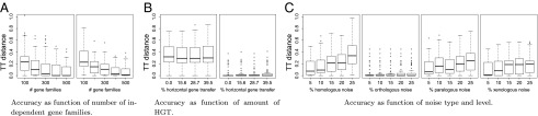
Accuracy of reconstructed species trees in simulated data sets. (A) Dependence on the number of gene families: 10 (Left) and 20 (Right) species and 100–500 gene families are generated using ALF with duplication/loss rate 0.005 and horizontal gene transfer rate 0.0. (B) Dependence on the intensity of horizontal gene transfer: Orthology estimated with Proteinortho (Left) and assuming perfect paralogy knowledge (Right); 10 species and 1,000 gene families are generated using ALF with duplication/loss rate 0.005 and horizontal gene transfer rate ranging from 0.0 to 0.0075. (C) Dependence on the type and intensity $\left(p=5-25\text{\%}\right)$ of noise in the raw orthology data $\mathrm{\Theta }$: 10 species and 1,000 gene families are generated using ALF with duplication/loss rate 0.005 and horizontal gene transfer rate 0.0. Tree distances are measured by the triple metric (TT); all box plots summarize 100 independent data sets.

To evaluate the robustness of the species trees in response to noise in the input data, we used simulated gene families with different noise models and levels: (i) insertion and deletion of edges in the orthology graph (homologous noise), (ii) insertion of edges (orthologous noise), (iii) deletion of edges (paralogous noise), and (iv) modification of gene/species assignments (xenologous noise). We observe a substantial dependence of the accuracy of the reconstructed species trees on the noise model. The results are most resilient against overprediction of orthology (noise model ii), whereas missing edges in $\mathrm{\Theta }$ have a larger impact; see Fig. 2C for TT distance, and SI Appendix for the other distances. This behavior can be explained by the observation that many false orthologs (overpredicting orthology) lead to an orthology graph, whose components are more clique-like and hence yield few informative triples. Incorrect species triples thus are reduced, whereas missing species triples often can be supplemented through other gene families. On the other hand, if there are many false paralogs (underpredicting orthology), more false species triples are introduced, resulting in inaccurate trees. Xenologous noise (model iv), simulated by changing gene/species associations with probability p while retaining the original gene tree, amounts to an extreme model for horizontal transfer. Our model, in particular in the weighted version, is quite robust for small amounts of HGT of 5–10%. Although some incorrect triples are introduced in the wake of horizontal transfer, they are usually dominated by correct alternatives observed from multiple gene families, and thus excluded during computation of the maximal consistent triple set. Only large-scale concerted horizontal transfer, which may occur in long-term endosymbiotic associations (39), thus poses a serious problem.

Simulations with ALF (37) show that our method is resilient against errors resulting from mispredicting xenology as orthology (see Fig. 2B, Right), even at horizontal gene transfer rates of $39.5\text{\%}$. Assuming perfect paralogy knowledge, i.e., assuming that all xenologs are mispredicted as orthologs, the correct trees are reconstructed essentially independently from the amount of HGT for $69.75\text{\%}$ of the data sets, and the triple distance to the correct tree remains minute in the remaining cases. This is consistent with noise model ii, i.e., a bias toward overpredicting orthology. Tree reconstructions based directly on the estimated orthology relation computed with Proteinortho are of course more inaccurate (Fig. 2B, Left). Even extreme rates of HGT, however, have no discernible effect on the quality of the inferred species trees. Our approach is therefore limited only by the quality of initial orthology prediction tools.

The fraction s of all triples obtained from the orthology relations that are retained in the final tree estimates serves as a quality measure similar in flavor to, e.g., the retention index of cladistics. Bootstrapping support values for individual nodes are readily computed by resampling either at the level of gene families or at the level of triples (see SI Appendix).

For the Aquificales data set, Proteinortho predicts 2,856 gene families, from which, 850 contain duplications. The reconstructed species tree (see Fig. 3; support $s=0.61$) is almost identical to the tree presented in ref. 40. All species are clustered correctly according to their taxonomic families. A slight difference refers to the two Sulfurihydrogenibium species not being directly clustered. These two species are very closely related. With only a few duplicates exclusively found in one of the species, the data were not sufficient for the approach to resolve this subtree correctly. Additionally, Hydrogenivirga sp. is misplaced next to Persephonella marina. This does not come as a surprise: Lechner et al. (40) already suspected that the data from this species was contaminated with material from Hydrogenothermaceae.

Fig. 3.

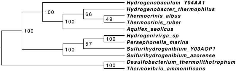
Phylogenetic tree of 11 Aquificales species inferred from paralogy. Internal node labels indicate triple-based bootstrap support.

The second data set comprises the genomes of 19 Enterobacteriales with 8,218 gene families, of which, 15 consist of more than 50 genes and 1,342 contain duplications. Our orthology-based tree shows the expected groupings of Escherichia and Shigella species and identifies the monophyletic groups comprising Salmonella, Klebsiella, and Yersinia species. The topology of the deeper nodes agrees only in part with the reference tree from PATRIC database (41); see SI Appendix for additional information. The resulting tree has a support of 0.53, reflecting that a few of the deeper nodes are poorly supported.

Data sets of around 20 species with a few thousand gene families, each having up to 50 genes, can be processed in reasonable time; see SI Appendix, Table S1. However, depending on the amount of noise in the data, the runtime for cograph editing can increase dramatically even for families with less than 50 genes.

Conclusion

We have shown here both theoretically and in a practical implementation that it is possible to access the phylogenetic information implicitly contained in gene duplications and thus to reconstruct a species phylogeny from information of paralogy only. This source of information is strictly complementary to the sources of information used in phylogenomics studies, which are always based on alignments of orthologous sequences. In fact, 1:1 orthologs—the preferred data in sequence-based phylogenetics—correspond to cographs that are complete and hence have a star as their cotree, and therefore do not contribute at all to the phylogenetic reconstruction in our approach. Access to the phylogenetic information implicit in (co)orthology data requires the solution of three NP-complete combinatorial optimization problems. This is generally the case in phylogenetics, however: Both the multiple sequence alignment problem and the extraction of maximum parsimony, maximum likelihood, or optimal Bayesian trees are NP-complete as well. Here we solve the computational tasks exactly for moderate-size problems by means of an ILP formulation. Using phylogenomic data for Aquificales and Enterobacteriales, we demonstrated that nontrivial phylogenies can indeed be reconstructed from tree-free orthology estimates alone. Just as sequence-based approaches in molecular phylogeny crucially depend on the quality of multiple sequence alignments, our approach is sensitive to the initial estimate $\mathrm{\Theta }$ of the orthology relation. Horizontal gene transfer, furthermore, is currently not included in the model but rather treated as noise that disturbs the phylogenetic signal. Simulated data indicate that the method is rather robust and can tolerate surprisingly large levels of noise in the form of both mispredicted orthology and horizontal gene transfer, provided a sufficient number of independent gene families is available as input data. Importantly, horizontal gene transfer can introduce a bias only when many gene families are simultaneously affected by horizontal transfer. Lack of duplications, on the other hand, limits our resolution at very short time scales, a regime in which sequence-based approaches work very accurately.

We have used here an exact implementation as ILP to demonstrate the potential of the approach without confounding it with computational approximations. Thus, the current implementation does not easily scale to very large data sets. Paralleling the developments in sequence-based phylogenetics, where the NP-complete problems of finding a good input alignment and of constructing tree(s) maximizing the parsimony score, likelihood, or Bayesian posterior probability also cannot be solved exactly for large data sets, it will be necessary, in practice, to settle for heuristic solutions. In sequence-based phylogenetics, these have improved over decades to the point where they are no longer a limiting factor in phylogenetic reconstruction. Several polynomial time heuristics and approximation algorithms have been devised already for the triple consistency problem (24, 42−44). The cograph-editing problem and the least resolved tree problem, in contrast, have received comparably little attention so far, but constitute the most obvious avenues for boosting computational efficiency. Empirical observations such as the resilience of our approach against overprediction of orthologs in the input will certainly be helpful in designing efficient heuristics.

In the long run, we envision that the species tree S and the symbolic representation of the event-annotated gene tree $\left(T,t\right)$ may serve as constraints for a refinement of the initial estimate of $\mathrm{\Theta }$, solely making use only of (nearly) unambiguously identified branchings and event assignments. A series of iterative improvements of estimates for $\mathrm{\Theta }$, $\left(T,t\right)$, and S, and, more importantly, methods that allow accurate detection of paralogs, may not only lead to more accurate trees and orthology assignments but could also turn out to be computationally more efficient.

References

- 1.Ebersberger I, Strauss S, von Haeseler A. HaMStR: Profile hidden Markov model based search for orthologs in ESTs. BMC Evol Biol. 2009;9:157. doi: 10.1186/1471-2148-9-157. [DOI] [PMC free article] [PubMed] [Google Scholar]
- 2.Fitch WM. Homology a personal view on some of the problems. Trends Genet. 2000;16(5):227–231. doi: 10.1016/s0168-9525(00)02005-9. [DOI] [PubMed] [Google Scholar]
- 3.Gabaldón T, Koonin EV. Functional and evolutionary implications of gene orthology. Nat Rev Genet. 2013;14(5):360–366. doi: 10.1038/nrg3456. [DOI] [PMC free article] [PubMed] [Google Scholar]
- 4.Altenhoff AM, Dessimoz C. Phylogenetic and functional assessment of orthologs inference projects and methods. PLOS Comput Biol. 2009;5(1):e1000262. doi: 10.1371/journal.pcbi.1000262. [DOI] [PMC free article] [PubMed] [Google Scholar]
- 5.Kristensen DM, Wolf YI, Mushegian AR, Koonin EV. Computational methods for gene orthology inference. Brief Bioinform. 2011;12(5):379–391. doi: 10.1093/bib/bbr030. [DOI] [PMC free article] [PubMed] [Google Scholar]
- 6.Dalquen DA, Altenhoff AM, Gonnet GH, Dessimoz C. The impact of gene duplication, insertion, deletion, lateral gene transfer and sequencing error on orthology inference: A simulation study. PLoS ONE. 2013;8(2):e56925. doi: 10.1371/journal.pone.0056925. [DOI] [PMC free article] [PubMed] [Google Scholar]
- 7.Böcker S, Dress AWM. Recovering symbolically dated, rooted trees from symbolic ultrametrics. Adv Math. 1998;138(1):105–125. [Google Scholar]
- 8.Hellmuth M, et al. Orthology relations, symbolic ultrametrics, and cographs. J Math Biol. 2013;66(1-2):399–420. doi: 10.1007/s00285-012-0525-x. [DOI] [PubMed] [Google Scholar]
- 9.Corneil DG, Lerchs H, Steward Burlingham L. Complement reducible graphs. Discrete Appl Math. 1981;3(3):163–174. [Google Scholar]
- 10.Liu Y, Wang J, Guo J, Chen J. Cograph editing: Complexity and parametrized algorithms. In: Fu B, Du DZ, editors. COCOON 2011, Lecture Notes on Computer Science. Vol 6842. Springer; Berlin: 2011. pp. 110–121. [Google Scholar]
- 11.Liu Y, Wang J, Guo J, Chen J. Complexity and parameterized algorithms for cograph editing. Theor Comput Sci. 2012;461(0):45–54. [Google Scholar]
- 12.Hernandez-Rosales M, et al. From event-labeled gene trees to species trees. BMC Bioinform. 2012;13(Suppl 19):S6. [Google Scholar]
- 13.Jansson J, Ng JH-K, Sadakane K, Sung W-K. Rooted maximum agreement supertrees. Algorithmica. 2005;43(4):293–307. [Google Scholar]
- 14.Guillemot S, Mnich M. Kernel and fast algorithm for dense triplet inconsistency. Theor Comput Sci. 2013;494:134–143. [Google Scholar]
- 15.Semple C. Reconstructing minimal rooted trees. Discrete Appl Math. 2003;127(3):489–503. [Google Scholar]
- 16.Jansson J, Lemence RS, Lingas A. The complexity of inferring a minimally resolved phylogenetic supertree. SIAM J Comput. 2012;41(1):272–291. [Google Scholar]
- 17.Bryant D. 1997. Building trees, hunting for trees, and comparing trees: theory and methods in phylogenetic analysis. PhD thesis (University of Canterbury, Christchurch, New Zealand)
- 18.Wu BY. Constructing the maximum consensus tree from rooted triples. J Comb Optim. 2004;8:29–39. [Google Scholar]
- 19.Jansson J. On the complexity of inferring rooted evolutionary trees. Electron Notes Discrete Math. 2001;7:50–53. [Google Scholar]
- 20.Dress AWM, Huber KT, Koolen J, Moulton V, Spillner A. Basic Phylogenetic Combinatorics. Cambridge Univ Press; Cambridge, UK: 2012. [Google Scholar]
- 21.Semple C, Steel M. Phylogenetics, Oxford Lecture Series in Mathematics and its Applications. Vol 24 Oxford Univ Press; Oxford: 2003. [Google Scholar]
- 22.Bininda-Emonds ORP. Phylogenetic Supertrees. Kluwer; Dordrecht, The Netherlands: 2004. [Google Scholar]
- 23.Aho AV, Sagiv Y, Szymanski TG, Ullman JD. Inferring a tree from lowest common ancestors with an application to the optimization of relational expressions. SIAM J Comput. 1981;10(3):405–421. [Google Scholar]
- 24.Byrka J, Gawrychowski P, Huber KT, Kelk S. Worst-case optimal approximation algorithms for maximizing triplet consistency within phylogenetic networks. J Discrete Alg. 2010;8(1):65–75. [Google Scholar]
- 25.Van Iersel L, Kelk S, Mnich M. Uniqueness, intractability and exact algorithms: Reflections on level-k phylogenetic networks. J Bioinform Comput Biol. 2009;7(4):597–623. doi: 10.1142/s0219720009004308. [DOI] [PubMed] [Google Scholar]
- 26.Byrka J, Guillemot S, Jansson J. New results on optimizing rooted triplets consistency. Discrete Appl Math. 2010;158(11):1136–1147. [Google Scholar]
- 27.Bryant D, Steel M. Extension operations on sets of leaf-labelled trees. Adv Appl Math. 1995;16(4):425–453. [Google Scholar]
- 28.Grünewald S, Steel M, Swenson MS. Closure operations in phylogenetics. Math Biosci. 2007;208(2):521–537. doi: 10.1016/j.mbs.2006.11.005. [DOI] [PubMed] [Google Scholar]
- 29.Huber KT, Moulton V, Semple C, Steel M. Recovering a phylogenetic tree using pairwise closure operations. Appl Math Lett. 2005;18(3):361–366. [Google Scholar]
- 30.Böcker S, Bryant D, Dress AWM, Steel MA. Algorithmic aspects of tree amalgamation. J Algorithms. 2000;37(2):522–537. [Google Scholar]
- 31.Dekker MCH. 1986. Reconstruction methods for derivation trees. Master’s thesis (Vrije Universiteit, Amsterdam)
- 32.Brandstädt A, Le VB, Spinrad JP. Graph Classes: A Survey, SIAM Monographs on Discrete Mathematics and Applications. Vol 3 Soc Ind Appl Math; Philadephia: 1999. [Google Scholar]
- 33.Corneil DG, Perl Y, Stewart LK. A linear recognition algorithm for cographs. SIAM J Comput. 1985;14(4):926–934. [Google Scholar]
- 34.Habib M, Paul C. A simple linear time algorithm for cograph recognition. Discrete Appl Math. 2005;145(2):183–197. [Google Scholar]
- 35.Chang W-C, Burleigh GJ, Fernández-Baca DF, Eulenstein O. An ILP solution for the gene duplication problem. BMC Bioinformatics. 2011;12(Suppl 1):S14. doi: 10.1186/1471-2105-12-S1-S14. [DOI] [PMC free article] [PubMed] [Google Scholar]
- 36.Hernandez-Rosales M, Hellmuth M, Wieseke N, Stadler PF. Simulation of gene family histories. BMC Bioinformatics. 2014;15(Suppl 3):A8. [Google Scholar]
- 37.Dalquen DA, Anisimova M, Gonnet GH, Dessimoz C. ALF—A simulation framework for genome evolution. Mol Biol Evol. 2012;29(4):1115–1123. doi: 10.1093/molbev/msr268. [DOI] [PMC free article] [PubMed] [Google Scholar]
- 38.Lechner M, et al. Proteinortho: Detection of (co-)orthologs in large-scale analysis. BMC Bioinformatics. 2011;12:124. doi: 10.1186/1471-2105-12-124. [DOI] [PMC free article] [PubMed] [Google Scholar]
- 39.Keeling PJ, Palmer JD. Horizontal gene transfer in eukaryotic evolution. Nat Rev Genet. 2008;9(8):605–618. doi: 10.1038/nrg2386. [DOI] [PubMed] [Google Scholar]
- 40.Lechner M, et al. Genomewide comparison and novel ncRNAs of Aquificales. BMC Genomics. 2014;15(1):522. doi: 10.1186/1471-2164-15-522. [DOI] [PMC free article] [PubMed] [Google Scholar]
- 41.Wattam AR, et al. PATRIC, the bacterial bioinformatics database and analysis resource. Nucleic Acids Res. 2014;42(Database issue, D1):D581–D591. doi: 10.1093/nar/gkt1099. [DOI] [PMC free article] [PubMed] [Google Scholar]
- 42.Gasieniec L, Jansson J, Lingas A, Ostlin A. On the complexity of constructing evolutionary trees. J Comb Optim. 1999;3(2-3):183–197. [Google Scholar]
- 43.Maemura K, Jansson J, Ono H, Sadakane K, Yamashita M. 2007. pp. 56–63. Approximation algorithms for constructing evolutionary trees from rooted triplets. Proceedings of 10th Korea-Japan Joint Workshop on Algorithms and Computation (Workshop on Algorithms and Computation, Gwangju, Korea), pp .
- 44.Tazehkand SJ, Hashemi SN, Poormohammadi H. New heuristics for rooted triplet consistency. Algorithms. 2013;6(3):396–406. [Google Scholar]
Associated Data
This section collects any data citations, data availability statements, or supplementary materials included in this article.